báo cáo hóa học:" Research Article Variable Viscosity on Magnetohydrodynamic Fluid Flow and Heat Transfer over an Unsteady Stretching Surface with Hall Effect" pot
Bạn đang xem bản rút gọn của tài liệu. Xem và tải ngay bản đầy đủ của tài liệu tại đây (775.16 KB, 20 trang )
Hindawi Publishing Corporation
Boundary Value Problems
Volume 2010, Article ID 257568, 20 pages
doi:10.1155/2010/257568
Research Article
Variable Viscosity on Magnetohydrodynamic
Fluid Flow and Heat Transfer over an Unsteady
Stretching Surface with Hall Effect
S. Shateyi
1
and S. S. Motsa
2
1
School of Mathematical and Natural Sciences, University of Venda, Private Bag X5050,
Thohoyandou 0950, South Africa
2
Department of Mathematics, University of Swaziland, Private Bag 4, Kwaluseni M201, Swaziland
Correspondence should be addressed to S. Shateyi,
Received 16 July 2010; Accepted 16 August 2010
Academic Editor: Vicentiu D. Radulescu
Copyright q 2010 S. Shateyi and S. S. Motsa. This is an open access article distributed under
the Creative Commons Attribution License, which permits unrestricted use, distribution, and
reproduction in any medium, provided the original work is properly cited.
The problem of magnetohydrodynamic flow and heat transfer of a viscous, incompressible, and
electrically conducting fluid past a semi-infinite unsteady stretching sheet is analyzed numerically.
The problem was studied under the effects of Hall currents, variable viscosity, and variable
thermal diffusivity. Using a similarity transformation, the governing fundamental equations are
approximated by a system of nonlinear ordinary differential equations. The resultant system of
ordinary differential equations is then solved numerically by the successive linearization method
together with the Chebyshev pseudospectral method. Details ofthe velocity and temperature fields
as well as the local skin friction and the local Nusselt number for various values of the parameters
of the problem are presented. It is noted that the axial velocity decreases with increasing the
values of the unsteadinessparameter, variable viscosity parameter, or theHartmann number, while
the transverse velocity increases as the Hartmann number increases. Due to increases in thermal
diffusivity parameter, temperature is found to increase.
1. Introduction
Fluid and heat flow induced by continuous stretching heated surfaces is often encountered in
many industrial disciplines. Applications include extrusion process, wire and fiber coating,
polymer processing, foodstuff processing, design of various heat exchangers, and chemical
processing equipment, among other applications. Stretching will bring in a unidirectional
orientation to the extrudate, consequently the quality of the final product considerably
depends on the flow and heat transfer mechanism. To that end, the analysis of momentum
and thermal transports within the fluid on a continuously stretching surface is important for
2 Boundary Value Problems
gaining some fundamental understanding of such processes. Since the pioneering study by
Crane 1 who presented an exact analytical solution for the steady two-dimensional flow
due to a stretching surface in a quiescent fluid, many studies on stretched surfaces have been
done. Dutta et al. 2 and Grubka and Bobba 3 studied the temperature field in the flow
over a stretching surface subject to a uniform heat flux.
Elbashbeshy 4 considered the case of a stretching surface with variable surface
heat flux. Chen and Char 5 presented an exact solution of heat transfer for a stretching
surface with variable heat flux. P. S. Gupta and A. S. Gupta 6 examined the heat and mass
transfer for the boundary layer flow over a stretching sheet subject to suction and blowing.
Elbashbeshy and Bazid 7 studied heat and mass transfer over an unsteady stretching
surface with internal heat generation.
Abd El-Aziz 8 analyzed the effect of radiation on heat and fluid flow over an
unsteady stretching surface. Mukhopadyay 9 performed an analysis to investigate the
effects of thermal radiation on unsteady boundary layer mixed convection heat transfer
problem from a vertical porous stretching surface embedded in porous medium. Recently,
Shateyi and Motsa 10 numerically investigated unsteady heat, mass, and fluid transfer over
a horizontal stretching sheet.
In all the above-mentioned studies, the viscosity of the fluid was assumed to be
constant. However, it is known that the fluid physical properties may change significantly
with temperature changes. To accurately predict the flow behaviour, it is necessary to
take into account this variation of viscosity with temperature. Recently, many researchers
investigated the effects of variable properties for fluid viscosity and thermal conductivity on
flow and heat transfer over a continuously moving surface.
Seddeek 11 investigated the effect of variable viscosity on hydromagnetic flow past a
continuously moving porous boundary. Seddeek 12 also studied the effect of radiation and
variable viscosity on an MHD free convection flow past a semi-infinite flat plate within an
aligned magnetic field in the case of unsteady flow. Dandapat et al. 13 analyzed the effects
of variable viscosity, variable thermal conducting, and thermocapillarity on the flow and heat
transfer in a laminar liquid film on a horizontal stretching sheet.
Mukhopadhyay 14 presented solutions for unsteady boundary layer flow and
heat transfer over a stretching surface with variable fluid viscosity and thermal diffusivity
in presence of wall suction. The study of magnetohydrodynamic flow of an electrically
conducting fluid is of considerable interest in modern metallurgical and great interest in
the study of magnetohydrodynamic flow and heat transfer in any medium due to the effect
of magnetic field on the boundary layer flow control and on the performance of many
systems using electrically conducting fluids. Many industrial processes involve the cooling
of continuous strips or filaments by drawing them through a quiescent fluid. During this
process, these strips are sometimes stretched. In these cases, the properties of the final product
depend to a great extent on the rate of cooling. By drawing these strips in an electrically
conducting fluid subjected to magnetic field, the rate of cooling can be controlled and the
final product of required characteristics can be obtained. Another important application of
hydromagnetics to metallurgy lies in the purification of molten metals from nonmetallic
inclusion by the application of magnetic field.
When the conducting fluid is an ionized gas and the strength of the applied magnetic
field is large, the normal conductivity of the magnetic field is reduced to the free spiraling
of electrons and ions about the magnetic lines force before suffering collisions and a current
is induced in a normal direction to both electric and magnetic field. This phenomenon is
called Hall effect. When the medium is a rare field or if a strong magnetic field is present,
Boundary Value Problems 3
the effect of Hall current cannot be neglected. The study of MHD viscous flows with
Hall current has important applications in problems of Hall accelerators as well as flight
magnetohydrodynamics.
Mahmoud 15 investigated the influence of radiation and temperature-dependent
viscosity on the problem of unsteady MHD flow and heat transfer of an electrically
conducting fluid past an infinite vertical porous plate taking into account the effect of
viscous dissipation. Tsai et al. 16 examined the simultaneous effects of variable viscosity,
variable thermal conductivity, and Ohmic heating on the fluid flow and heat transfer past a
continuously moving porous surface under the presence of magnetic field. Abo-Eldahab and
Abd El-Aziz 17 presented an analysis for the effects of viscous dissipation and Joule heating
on the flow of an electrically conducting and viscous incompressible fluid past a semi-infinite
plate in the presence of a strong transverse magnetic field and heat generation/absorption
with Hall and ion-slip effects. Abo-Eldahab et al. 18 and Salem and Abd El-Aziz 19 dealt
with the effect of Hall current on a steady laminar hydromagnetic boundary layer flow of an
electrically conducting and heat generating/absorbing fluid along a stretching sheet.
Pal and Mondal 20 investigated the effect of temperature-dependent viscosity on
nonDarcy MHD mixed convective heat transfer past a porous medium by taking into account
Ohmic dissipation and nonuniform heat source/sink. Abd El-Aziz 21 investigated the effect
of Hall currents on the flow and heat transfer of an electrically conducting fluid over an
unsteady stretching surface in the presence of a strong magnet.
The present paper deals with variable viscosity on magnetohydrodynamic fluid
and heat transfer over an unsteady stretching surface with Hall effect. Fluid viscosity
is assumed to vary as an exponential function of temperature while the fluid thermal
diffusivity is assumed to vary as a linear function of temperature. Using appropriate
similarity transformation, the unsteady Navier-Stokes equations along with the energy
equation are reduced to a set of coupled ordinary differential equations. These equations
are then numerically solved by successive linearization method. The effects of different
parameters on velocity and temperature fields are investigated and analyzed with the help
of their graphical representations along with the energy.
2. Mathematical Formulation
We consider the unsteady flow and heat transfer of a viscous, incompressible, and electrically
conducting fluid past a semi-infinite stretching sheet coinciding with the plane y 0, then
the fluid is occupied above the sheet y ≥ 0. The positive x coordinate is measured along
the stretching sheet in the direction of motion, and the positive y coordinate is measured
normally to the sheet in the outward direction toward the fluid. The leading edge of the
stretching sheet is taken as coincident with z-axis. The continuous sheet moves in its own
plane with velocity U
w
x, t, and the temperature T
w
x, t distribution varies both along
the sheet and time. A strong uniform magnetic field is applied normally to the surface
causing a resistive force in the x-direction. The stretching surface is maintained at a constant
temperature and with significant Hall currents. The magnetic Reynolds number is assumed
to be small so that the induced magnetic field can be neglected. The effect of Hall current
gives rise to a force in the z-direction, which induces a cross flow in that direction, and hence
the flow becomes three dimensional. To simplify the problem, we assume that there is no
variation of flow quantities in z-direction. This assumption is considered to be valid if the
surface is of infinite extent in the z-direction. Further, it is assumed that the Joule heating and
viscous dissipation are neglected in this study. Finally, we assume that the fluid viscosity is
4 Boundary Value Problems
to vary with temperature while other fluid properties are assumed to be constant. Using
boundary layer approximations, the governing equations for unsteady laminar boundary
layer flows are written as follows:
∂u
∂x
∂v
∂y
0,
2.1
∂u
∂t
u
∂u
∂x
v
∂u
∂y
1
ρ
∂
∂y
μ
∂u
∂y
−
σB
2
ρ
1 m
2
u mw
, 2.2
∂w
∂t
u
∂w
∂x
v
∂w
∂y
1
ρ
∂
∂y
μ
∂w
∂y
σB
2
ρ
1 m
2
mu − w
, 2.3
∂T
∂t
u
∂T
∂x
v
∂T
∂y
1
ρc
p
∂
∂y
k
∂T
∂y
,
2.4
subject to the following boundary conditions:
u U
w
x, t
,v 0,w 0,T T
w
x, t
, at y 0,
u −→ 0,w−→ 0,T−→ T
∞
, as y −→ ∞,
2.5
where u and v are the velocity components along the x-andy-axis, respectively, w is the
velocity component in the z direction, ρ is the fluid density, β is the coefficient of thermal
expansion, μ is the kinematic viscosity, g is the acceleration due to gravity, c
p
is the specific
heat at constant pressure, and k is the temperature-dependent thermal conductivity.
Following Elbashbeshy and Bazid 22, we assume that the stretching velocity U
w
x, t
is to be of the following form:
U
w
bx
1 − ct
, 2.6
where b and c are positive constants with dimension reciprocal time. Here, b is the initial
stretching rate, whereas the effective stretching rate b/1 − ct is increasing with time. In the
context of polymer extrusion, the material properties and in particular the elasticity of the
extruded sheet vary with time even though the sheet is being pulled by a constant force.
With unsteady stretching, however, c
−1
becomes the representative time scale of the resulting
unsteady boundary layer problem.
The surface temperature T
w
of the stretching sheet varies with the distance x along the
sheet and time t in the following form:
T
w
x, t
T
∞
T
0
bx
2
ν
∗
1 − αt
−3/2
, 2.7
where T
0
is a positive or negative; heating or cooling reference temperature.
Boundary Value Problems 5
The governing differential equations 2.1–2.4 together with the boundary condi-
tions 2.5 are nondimensionalized and reduced to a system of ordinary differential equations
using the following dimensionless variables:
η
b
ν
1/2
1 − αt
−1/2
y, ψ
νb
1/2
1 − αt
−1/2
xf
η
,w bx
1 − ct
−1
h
η
,
T T
∞
T
0
bx
2
2ν
1 − αt
−
3
2
θ
η
,B
2
B
2
0
1 − ct
−1
,
2.8
where ψx, y, t is the physical stream function which automatically assures mass conserva-
tion 2.1 and B
0
is constant.
We assume the fluid viscosity to vary as an exponential function of temperature in
the nondimensional form μ μ
∞
e
−β
1
θ
, where μ
∞
is the constant value of the coefficient of
viscosity far away from the sheet, β
1
is the variable viscosity parameter. The variation of
thermal diffusivity with the dimensionless temperature is written as k k
0
1β
2
θ, where β
2
is a parameter which depends on the nature of the fluid, k
0
is the value of thermal diffusivity
at the temperature T
w
.
Upon substituting the above transformations into 2.1–2.4 we obtain the following:
f
− β
1
θ
f
e
β
1
θ
ff
−
f
2
− S
f
η
2
f
−
M
2
1 m
2
f
mh
0, 2.9
h
− β
1
θ
h
e
β
1
θ
fh
− hf
− S
h
η
2
h
M
2
1 m
2
mf
− h
0, 2.10
1 β
2
θ
θ
β
2
θ
2
Pr
fθ
− 2f
θ
− S
3θ ηθ
0, 2.11
where the primes denote differentiation with respect to η, and the boundary conditions are
reduced to
f
0
0,f
0
1,h
0
0,θ
0
1, 2.12
h
∞
0,f
∞
0,θ
∞
0. 2.13
The governing nondimensional equations 2.9–2.11 along with the boundary conditions
2.12-2.13 are solved using a numerical perturbation method referred to as the method of
successive linearisation.
6 Boundary Value Problems
3. Successive Linearisation Method (SLM)
The SLM algorithm starts with the assumption that the independent variables fη, hη,and
θη can be expressed as follows:
f
η
F
i
η
i−1
n0
f
n
η
,h
η
H
i
η
i−1
n0
h
n
η
,θ
η
G
i
η
i−1
n0
θ
n
η
,
3.1
where F
i
, H
i
, G
i
i 1, 2, 3, are unknown functions and f
n
, h
n
,andθ
n
n ≥ 1 are
approximations which are obtained by recursively solving the linear part of the equation
system that results from substituting 3.1 in the governing equations 2.9–2.13. The main
assumption of the SLM is that F
i
, G
i
,andH
i
become increasingly smaller when i becomes
large, that is,
lim
i →∞
F
i
lim
i →∞
G
i
lim
i →∞
H
i
0. 3.2
Thus, starting from the initial guesses f
0
η, h
0
η,andθ
0
η,
f
0
η
1 − e
−η
,h
0
η
0,θ
0
η
e
−η
, 3.3
which are chosen to satisfy the boundary conditions 2.12 and 2.13, the subsequent
solutions for f
i
,h
i
,θ
i
, i ≥ 1 are obtained by successively solving the linearised form of
equations which are obtained by substituting 3.1 in the governing equations, considering
only the linear terms. In view of the assumption 3.2, the exponential term e
β
1
θ
can be
approximated as follows:
e
β
1
θ
exp
β
i−1
n0
θ
n
· exp βG
i
≈ exp
β
i−1
n0
θ
n
1 βG
i
···
. 3.4
Thus, using 3.4, the linearised equations to be solved are given as follows:
f
i
a
1,i−1
f
i
a
2,i−1
f
i
a
3,i−1
f
i
a
4,i−1
f
i
a
5,i−1
θ
i
a
6,i−1
θ
i
r
i−1
,
h
i
b
1,i−1
h
i
b
2,i−1
h
i
b
3,i−1
f
i
b
4,i−1
f
i
b
5,i−1
θ
i
b
6,i−1
θ
i
s
i−1
,
c
1,i−1
θ
i
c
2,i−1
θ
i
c
3,i−1
θ
i
c
4,i−1
f
i
c
5,i−1
f
i
t
i−1
,
3.5
subject to the boundary conditions
f
i
0
f
i
0
f
i
∞
h
i
0
h
i
∞
θ
i
0
θ
i
∞
0, 3.6
where the coefficient parameters a
k,i−1
, b
k,i−1
, c
k,i−1
k 1, ,6, r
i−1
, s
i−1
,andt
i−1
are defined
in the appendix.
Boundary Value Problems 7
Once each solution for f
i
, h
i
,andθ
i
i ≥ 1 has been found from iteratively solving
3.5, the approximate solutions for fη, hη,andθη are obtained as follows:
f
η
≈
K
n0
f
n
η
,f
η
≈
K
n0
h
n
η
,θ
η
≈
K
n0
θ
n
η
, 3.7
where K is the order of SLM approximation. Since the coefficient parameters and the right-
hand side of 3.5,fori 1, 2, 3, , are known from previous iterations, the equation
system 3.5 can easily be solved using any numerical methods such as finite differences,
finite elements, Runge-Kutta-based shooting methods, or collocation methods. In this work,
3.5 are solved using the Chebyshev spectral collocation method. This method is based on
approximating the unknown functions by the Chebyshev interpolating polynomials in such
a way that they are collocated at the Gauss-Lobatto points defined as follows:
ξ
j
cos
πj
N
,j 0, 1, ,N, 3.8
where N is the number of collocation points used see e.g. 23–25. In order to implement
the method, the physical region 0, ∞ is transformed into the region −1, 1 using the domain
truncation technique in which the problem is solved on the interval 0,L instead of 0, ∞.
This leads to the following mapping:
η
L
ξ 1
2
, −1 ≤ ξ ≤ 1, 3.9
where L is the scaling parameter used to invoke the boundary condition at infinity. The
unknown functions f
i
and θ
i
are approximated at the collocation points by
f
i
ξ
≈
N
k0
f
i
ξ
k
T
k
ξ
j
,h
i
ξ
≈
N
k0
h
i
ξ
k
T
k
ξ
j
,θ
i
ξ
≈
N
k0
θ
i
ξ
k
T
k
ξ
j
,j0, 1, ,N,
3.10
where T
k
is the kth Chebyshev polynomial defined as follows:
T
k
ξ
cos
k cos
−1
ξ
. 3.11
The derivatives of the variables at the collocation points are represented as follows:
d
a
f
i
dη
a
N
k0
D
a
kj
f
i
ξ
k
,
d
a
h
i
dη
a
N
k0
D
a
kj
h
i
ξ
k
,
d
a
θ
i
dη
a
N
k0
D
r
kj
θ
i
ξ
k
,j 0, 1, ,N, 3.12
8 Boundary Value Problems
where a is the order of differentiation and D 2/LD with D being the Chebyshev spectral
differentiation matrix see e.g., 23, 25. Substituting 3.9–3.12 in 3.5 leads to the matrix
equation given as follows:
A
i−1
X
i
R
i−1
, 3.13
in which A
i−1
is a 3N 3 × 3N 3 square matrix and X and R are 3N 1 × 1 column
vectors defined by
A
i−1
⎡
⎣
A
11
A
12
A
13
A
21
A
22
A
23
A
31
A
32
A
33
⎤
⎦
, X
i
⎡
⎣
F
i
H
i
Θ
i
⎤
⎦
, R
i−1
⎡
⎣
r
i−1
s
i−1
t
i−1
⎤
⎦
, 3.14
in which
F
i
f
i
ξ
0
,f
i
ξ
1
, ,f
i
ξ
N−1
,f
i
ξ
N
T
,
H
i
h
i
ξ
0
,h
i
ξ
1
, ,h
i
ξ
N−1
,h
i
ξ
N
T
,
Θ
i
θ
i
ξ
0
,θ
i
ξ
1
, ,θ
i
ξ
N−1
,θ
i
ξ
N
T
,
r
i−1
r
i−1
ξ
0
,r
i−1
ξ
1
, ,r
i−1
ξ
N−1
,r
i−1
ξ
N
T
,
s
i−1
s
i−1
ξ
0
,s
i−1
ξ
1
, ,s
i−1
ξ
N−1
,s
i−1
ξ
N
T
,
t
i−1
t
i−1
ξ
0
,t
i−1
ξ
1
, ,t
i−1
ξ
N−1
,t
i−1
ξ
N
T
,
3.15
and A
ij
i, j 1, 2, 3 are defined in the appendix. After modifying the matrix system 3.13 to
incorporate boundary conditions, the solution is obtained as follows:
X
i
A
−1
i−1
R
i−1
.
3.16
4. Results and Discussion
In this section, we give the SLM results for the six main parameters affecting the flow.
We remark that all the SLM results presented in this paper were obtained using N 30
collocation points. For validation, the SLM results were compared to those by Matlab routine
bvp4c and excellent agreement between the results is obtained giving the much needed
confidence in using the successive linearization method. Tables 1–3 give a comparison of
the SLM results for −f
0 and −θ
0 at different orders of approximation against the bvp4c.
In Table 1, we observe that full convergence of the SLM is achieved by as early as the third
order, substantiating the claim that SLM is a very powerful technique. We observe in this
table that the variable viscosity parameter β
1
significantly affects the skin friction −f
0. The
skin friction increases as β
1
increases. We observe also in this table that the local Nusselt
number −θ
0 decreases as the fluid variable viscosity parameter β
1
increases. The lower
part of Table 1 depicts the effects of variable diffusivity parameter β
2
on the local skin friction
−f
0 and the local Nusselt number −θ
0. It can be observed that β
2
does not have
Boundary Value Problems 9
0
0.1
0.2
0.3
0.4
0.5
0.6
0.7
0.8
0.9
1
f
η
012345678
η
β
1
0
β
1
0.4
β
1
1
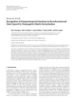
Figure 1: The variation axial velocity distributions with increasing values of β
1
with M 1, Pr 0.72,
m 1, β
2
0.1, and S 0.8.
significant effect on the skin friction but very significant effects on the local Nusselt number.
As β
2
increases, the skin friction slightly decreases but the local Nusselt number is greatly
reduced.
From Table 2 upper part, it is observed that the Hartmann number M tends to
greatly increase the local skin friction at the unsteady stretching surface. This is because
the increase in the magnetic strength leads to a thinner boundary layer, thereby causing an
increase in the velocity gradient at the wall. We also observe that the local Nusselt number
decreases as the values of M increase. We observe in the lower part of Table 2 that the local
skin friction −f
0 is reduced as the Hall parameter m increases, but the Nusselt number
increases as m increases.
Table 3 depicts the effects of the unsteadiness parameter S, upper part the Prandtl
number Pr lower part on the local skin friction, and the local Nusselt number. We observe
that both of these flow properties are greatly affected by the unsteadiness parameter. They
both increase as the values of S increase. We also observe in this table that the Prandtl number
has little effects on the skin friction but significant effects on the local Nusselt number. The
local skin friction slightly increases as the values of the Prandtl number increase, while the
Nusselt number is greatly increased as Pr increases.
Figures 1–12 have been plotted to clearly depict the influence of various physical
parameters on the velocity and temperature distributions. In Figure 1,wehavetheeffects
of varying the variable viscosity parameter β
1
on the axial velocity. It is clearly seen that as
β
1
increases the boundary layer thickness decreases and the velocity distributions become
shallow. Physically, this is because a given larger fluid β
1
implies higher temperature
difference between the surface and the ambient fluid.
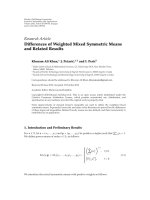
The effects of the unsteadiness parameter S on the axial velocity f
η are presented
in Figure 2. It can be seen in this figure that when S values are increased, the boundary layer
thickness is reduced and this inhibits the development of transition of laminar to turbulent
10 Boundary Value Problems
Tab le 1: Comparison between the present successive linearisation method SLM results and the bvp4c
numerical results for −f
0 and −θ0 for various values of β
1
and β
2
when Pr 0.72; M 1;m 1; S 0.8.
−f
0 −θ
0
β
2
0.1
β
1
2nd ord. 3rd ord. 4th ord. bvp4c 2nd ord. 3rd ord. 4th ord. bvp4c
0.1 1.554880 1.554902 1.554902 1.554902 1.270615 1.270618 1.270618 1.270618
0.2 1.654744 1.654780 1.654780 1.654780 1.262638 1.262637 1.262637 1.262637
0.3 1.759494 1.759550 1.759550 1.759550 1.254515 1.254506 1.254506 1.254506
0.4 1.869278 1.869358 1.869358 1.869358 1.246255 1.246233 1.246233 1.246233
0.5 1.984248 1.984356 1.984356 1.984356 1.237868 1.237829 1.237829 1.237829
0.6 2.104569 2.104702 2.104702 2.104702 1.229367 1.229305 1.229305 1.229305
β
1
0.1
β
2
2nd ord. 3rd ord. 4th ord. bvp4c 2nd ord. 3rd ord. 4th ord. bvp4c
0.1 1.554880 1.554902 1.554902 1.554902 1.270615 1.270618 1.270618 1.270618
0.2 1.554140 1.554159 1.554159 1.554159 1.196543 1.196541 1.196541 1.196541
0.3 1.553464 1.553482 1.553482 1.553482 1.132811 1.132803 1.132803 1.132803
0.4 1.552845 1.552861 1.552861 1.552861 1.077289 1.077278 1.077278 1.077278
0.5 1.552274 1.552289 1.552289 1.552289 1.028406 1.028392 1.028392 1.028392
0.6 1.551747 1.551761 1.551761 1.551761 0.984976 0.984958 0.984958 0.984958
Tab le 2: Comparison between the present successive linearisation method SLM results and the bvp4c
numerical results for −f
0 and −θ0 for various values of M and m when Pr 0.72; M 1;m 1;S
0.8.
−f
0 −θ
0
m 1
M 2nd ord. 3rd ord. 4th ord. bvp4c 2nd ord. 3rd ord. 4th ord. bvp4c
0.1 1.346973 1.346977 1.346977 1.346977 1.298217 1.298219 1.298219 1.298219
1.0 1.554880 1.554902 1.554902 1.554902 1.270615 1.270618 1.270618 1.270618
2.0 2.094695 2.094728 2.094728 2.094728 1.205903 1.205873 1.205873 1.205873
3.0 2.780752 2.780758 2.780758 2.780758 1.142601 1.142533 1.142533 1.142533
4.0 3.524973 3.524963 3.524963 3.524963 1.092001 1.091925 1.091925 1.091925
5.0 4.296202 4.296187 4.296187 4.296187 1.052905 1.052838 1.052838 1.052838
6.0 5.081869 5.081855 5.081855 5.081855 1.022458 1.022404 1.022404 1.022404
M 1
m 2nd ord. 3rd ord. 4th ord. bvp4c 2nd ord. 3rd ord. 4th ord. bvp4c
0.1 1.711146 1.711172 1.711172 1.711172 1.254049 1.254052 1.254052 1.254052
1.0 1.554880 1.554902 1.554902 1.554902 1.270615 1.270618 1.270618 1.270618
2.0 1.438664 1.438677 1.438677 1.438677 1.285089 1.285092 1.285092 1.285092
3.0 1.394031 1.394040 1.394040 1.394040 1.291251 1.291254 1.291254 1.291254
4.0 1.374422 1.374429 1.374429 1.374429 1.294079 1.294082 1.294082 1.294082
5.0 1.364411 1.364417 1.364417 1.364417 1.295553 1.295556 1.295556 1.295556
6.0 1.358689 1.358695 1.358695 1.358695 1.296405 1.296408 1.296408 1.296408
flow. The effect of the magnetic strength parameter M on the axial velocity f
η is shown
in Figure 3. It is noticed that an increase in the magnetic parameter leads to a decrease in
the velocity. This is due to the fact that the application of the transverse magnetic field to an
electrically conducting fluid gives rise to a resistive type of force known as the Lorentz force.
This force has a tendency to slow the motion of the fluid in the axial direction.
Boundary Value Problems 11
Tab le 3: Comparison between the present successive linearisation method SLM results and the bvp4c
numerical results for −f
0 and −θ0 for various values of S and Pr when β
1
0.1,β
2
0.1,M 1; m
1; S 0.8.
−f
0 −θ
0
Pr 0.72
S 2nd ord. 3rd ord. 4th ord. bvp4c 2nd ord. 3rd ord. 4th ord. bvp4c
0.1 1.356050 1.356062 1.356062 1.356062 0.982230 0.981936 0.981936 0.981936
0.5 1.471732 1.471752 1.471752 1.471752 1.161685 1.161666 1.161666 1.161666
1.0 1.608655 1.608677 1.608677 1.608677 1.336560 1.336569 1.336569 1.336569
1.5 1.737464 1.737489 1.737489 1.737489 1.485834 1.485849 1.485849 1.485849
2.5 1.973469 1.973500 1.973500 1.973500 1.741847 1.741866 1.741866 1.741866
3.0 2.082331 2.082365 2.082365 2.082365 1.855701 1.855719 1.855719 1.855719
S 0.8
Pr 2nd ord. 3rd ord. 4th ord. bvp4c 2nd ord. 3rd ord. 4th ord. bvp4c
0.1 1.542490 1.542494 1.542494 1.542494 0.405270 0.405254 0.405254 0.405254
0.5 1.551892 1.551905 1.551905 1.551905 1.032273 1.032252 1.032252 1.032252
1.0 1.557830 1.557862 1.557862 1.557862 1.529016 1.529053 1.529053 1.529053
1.5 1.561763 1.561812 1.561812 1.561812 1.916129 1.916220 1.916220 1.916220
2.5 1.567062 1.567138 1.567138 1.567138 2.535077 2.535240 2.535240 2.535240
3.0 1.569013 1.569099 1.569099 1.569099 2.798249 2.798436 2.798436 2.798436
0
0.1
0.2
0.3
0.4
0.5
0.6
0.7
0.8
0.9
1
f
η
0123456
η
S 1
S 3
S 5
S 8
Figure 2: The variation axial velocity distributions with increasing values of S with M 1, Pr 0.72,
m 1, β
1
0.1, and β
2
0.1.
Figure 4 shows typical profiles for the fluid velocity f
η for different values of the
Hall parameter m. We observe that f
η increases with increasing values of m as the effective
conducting σ/1 m
2
decreases with increasing m which reduces the magnetic damping
force on f
η, and the reduction in the magnetic damping force is coupled with the fact that
magnetic field has a propelling effect on f
η.
12 Boundary Value Problems
0
0.1
0.2
0.3
0.4
0.5
0.6
0.7
0.8
0.9
1
f
η
012345678
η
M 1
M 2
M 4
M 6
Figure 3: The variation axial velocity distributions with increasing values of M with Pr 0.72, m 1,
β
1
0.1, β
2
0.1, and S 0.8.
0
0.1
0.2
0.3
0.4
0.5
0.6
0.7
0.8
0.9
1
f
η
012345678
η
m 2
m 4
m 6
Figure 4: The variation axial velocity distributions with increasing values of m with M 1, Pr 0.72,
β
1
0.1, β
2
0.1, and S 0.8.
Figure 5 shows the effect of the variable viscosity parameter β
1
on the transverse
velocity distribution hη. As shown, the velocity is decreasing with increasing the values
of β
1
. In addition, the curves show that for a particular value of β
1
, the transverse velocity
increases rapidly to a peak value near the wall and then decays to the relevant free stream
velocity zero.Theeffect of the unsteadiness parameter S on the transverse velocity hη is
Boundary Value Problems 13
0
0.01
0.02
0.03
0.04
0.05
0.06
hη
02468101214161820
η
β
1
0
β
1
0.4
β
1
1
Figure 5: Transverse velocity profiles for various values of β
1
with M 1, Pr 0.72, m 1, β
2
0.1, and
S 0.8.
0
0.01
0.02
0.03
0.04
0.05
0.06
hη
02468101214
η
S 1
S 3
S 5
S 8
Figure 6: Transverse velocity profiles for various values of S with M 1, Pr 0.72, m 1, β
1
0.1, and
β
2
0.1.
presented in Figure 6. From this figure, it is seen that the effect of increasing the unsteadiness
parameter S is to decrease the transverse velocity hη greatly near the plate.
Figure 7 depicts the effects of the magnetic strength M on the transverse velocity. We
observe that close to the sheet surface an increase in the values of M leads to an increase
in the values of the transverse velocity with shifting the maximum values toward the plate
14 Boundary Value Problems
0
0.02
0.04
0.06
0.08
0.1
0.12
0.14
0.16
hη
012345678
η
M 1
M 2
M 4
M 6
Figure 7: Transverse velocity profiles for various values of M with β
1
0.1, Pr 0.72, m 1, β
2
0.1, and
S 0.8.
0
0.01
0.02
0.03
0.04
0.05
0.06
hη
02468101214161820
η
m 1.5
m 2
m 0.7
m 0.5
m 4
m 6
Figure 8: Transverse velocity profiles for various values of m with M 1, Pr 0.72, β
1
0.1, β
2
0.1, and
S 0.8.
while for most of the parts of the boundary layer at the fixed η position, the transverse
velocity decreases along with decreases in the boundary layer thickness as the magnetic field
increases.
Figure 8 is obtained by fixing the values of all the parameters and by allowing the Hall
parameter m to vary. Increasing the values of m from 0 to 1.5 causes the transverse flow in
the z-direction to increase. However, for values of m greater than 1.5, the transverse flow
decreases as these values increase as can be clearly seen on Figure 8. This is due to the fact
Boundary Value Problems 15
0
0.1
0.2
0.3
0.4
0.5
0.6
0.7
0.8
0.9
1
θη
012345678910
η
β
1
0
β
1
0.4
β
1
1
Figure 9: Temperature profiles for various values of β
1
with M 1, Pr 0.72, m 1, β
2
0.1, and S 0.8.
0
0.1
0.2
0.3
0.4
0.5
0.6
0.7
0.8
0.9
1
θη
012345678910
η
β
2
0
β
2
0.4
β
2
1
Figure 10: Temperature profiles for various values of β
2
with M 1, Pr 0.72, m 1, β
1
0.1, and S 0.8.
that for larger values of m, the term σ/1 m
2
is very small, and hence the resistive effect of
the magnetic field is diminished.
Figures 9 and 10 are aimed to shed light on the effects of variable viscosity and
variable thermal diffusivity parameters β
1
and β
2
on the temperature. The distribution θη
increases as β
1
and β
2
increase as shown in Figure 9 and Figure 10, respectively. This is due
to the thickening of the thermal boundary layer as a result of increasing thermal diffusivity.
16 Boundary Value Problems
0
0.1
0.2
0.3
0.4
0.5
0.6
0.7
0.8
0.9
1
θη
012345678910
η
S 1
S 3
S 5
S 8
Figure 11: Temperature profiles for various values of S with M 1, Pr 0.72, m 1, β
2
0.1, and β
1
0.1.
0
0.1
0.2
0.3
0.4
0.5
0.6
0.7
0.8
0.9
1
θη
012345678910
η
M 1
M 2
M 4
M 6
Figure 12: Temperature profiles for various values of M with S 1, Pr 0.72, m 1, β
2
0.1, and β
1
0.1.
Figure 11 depicts the effect of the unsteadiness parameter S on the temperature profiles. It
can be observed that the temperature profiles decrease with the increase of S. In general, it is
noted that the effect of S on hη and θη is more notable than that on f
η.
Figure 12 presents typical profiles for the fluid temperature θη for different values
of Hartmann number M. Increases in the values of M have a tendency to slow the motion
of the fluid and make it warmer as it moves along the unsteady stretching sheet causing θ to
increase as shown in this figure.
Boundary Value Problems 17
5. Conclusion
The problem of unsteady magnetohydrodynamic flow and heat transfer of a viscous,
incompressible, and electrically conducting fluid past a semi-infinite stretching sheet was
investigated. The governing continuum equations that comprised the balance laws of mass,
linear momentum, and energy were modified to include the Hartmann and Hall effects of
magnetohydrodynamics, and variable viscosity of the fluid was solved numerically using the
successive linearization method together with the Chebyshev collocation method. Graphical
results for the velocity and temperature were presented and discussed for various physical
parametric values. The effects of the main physical parameters of the problem on the skin
friction and the local Nusselt number were shown in Tabular form. It was found that the
skin coefficient −f
0 is increased as the variable viscosity parameter, Hartmann number,
unsteadiness parameter, or the Prandtl number is increased. It was found, however, to
decrease as the thermal diffusivity parameter or the Hall parameter increases. The local
Nusselt number −θ
0 was found to be decreasing as the values of the variable viscosity
parameter, thermal diffusivity parameter, or Hartmann number increase and to be increasing
with increasing the values of the Hall parameter, unsteadiness parameter, or the Prandtl
number.
It is hoped that, with the help of our present model, the physics of flow over stretching
sheet may be utilized as the basis of many scientific and engineering applications and
experimental work.
Appendix
A. Definition of Coefficient Parameters
a
1,i−1
−β
1
i−1
n0
θ
n
exp
β
1
i−1
n0
θ
n
i−1
n0
f
n
−
Sη
2
,
a
2,i−1
exp
β
1
i−1
n0
θ
n
−2
i−1
n0
f
n
− S −
M
2
1 m
2
,
a
3,i−1
exp
β
1
i−1
n0
θ
n
i−1
n0
f
n
,
a
4,i−1
exp
β
1
i−1
n0
θ
n
−
M
2
m
1 m
2
,
a
5,i−1
−β
1
i−1
n0
f
n
,
a
6,i−1
β
1
exp
β
1
i−1
n0
θ
n
⎡
⎣
i−1
n0
f
n
i−1
n0
f
n
−
i−1
n0
f
n
2
− S
i−1
n0
f
n
η
2
i−1
n0
f
n
−
M
2
1 m
2
i−1
n0
f
n
m
i−1
n0
h
n
,
r
i−1
−
i−1
n0
f
n
β
1
i−1
n0
θ
n
i−1
n0
f
n
−
1
β
1
a
6,i−1
,
A.1
18 Boundary Value Problems
b
1,i−1
−β
1
i−1
n0
θ
n
exp
β
1
i−1
n0
θ
n
i−1
n0
f
n
−
Sη
2
,
b
2,i−1
exp
β
1
i−1
n0
θ
n
−
i−1
n0
f
n
− S −
M
2
1 m
2
,
b
3,i−1
exp
β
1
i−1
n0
θ
n
−
i−1
n0
h
n
M
2
m
1 m
2
,
b
4,i−1
exp
β
1
i−1
n0
θ
n
i−1
n0
h
n
,
b
5,i−1
−β
1
i−1
n0
h
n
,
b
6,i−1
β
1
exp
β
1
i−1
n0
θ
n
i−1
n0
f
n
i−1
n0
h
n
−
i−1
n0
f
n
i−1
n0
h
n
− S
i−1
n0
h
n
η
2
i−1
n0
h
n
M
2
1 m
2
m
i−1
n0
f
n
−
i−1
n0
h
n
,
s
i−1
−
i−1
n0
h
n
β
1
i−1
n0
θ
n
i−1
n0
h
n
−
1
β
1
b
6,i−1
,
A.2
c
1,i−1
1 β
2
i−1
n0
θ
n
,
c
2,i−1
2β
2
i−1
n0
θ
n
Pr
i−1
n0
f
n
−
SPrη
2
,
c
3,i−1
β
2
i−1
n0
θ
n
− 2Pr
i−1
n0
f
n
−
3SPr
2
,
c
4,i−1
−2Pr
i−1
n0
θ
n
,
c
5,i−1
Pr
i−1
n0
θ
n
,
t
i−1
−
⎡
⎣
1 β
2
i−1
n0
θ
n
i−1
n0
θ
n
β
2
i−1
n0
θ
n
2
Pr
i−1
n0
f
n
i−1
n0
θ
n
− 2
i−1
n0
f
n
i−1
n0
θ
n
−
SPr
2
3
i−1
n0
θ
n
η
i−1
n0
θ
n
,
A.3
Boundary Value Problems 19
A
11
D
3
a
1,i−1
D
2
a
2,i−1
D a
3,i−1
,
A
12
a
4,i−1
,
A
13
a
5,i−1
D a
6,i−1
,
A
21
b
3,i−1
D b
4,i−1
,
A
22
D
2
b
1,i−1
D b
2,i−1
,
A
23
b
5,i−1
D b
6,i−1
,
A
31
c
4,i−1
D c
5,i−1
,
A
32
O, square matrix of zeros of order N 1,
A
33
c
1,i−1
D
2
c
2,i−1
D c
3,i−1
.
A.4
In the above definitions, a
k,i−1
, b
k,i−1
,andc
k,i−1
k 1, ,6 are diagonal matrices of size
N 1 × N 1.
References
1 L. J. Crane, “Flow past a stretching plate,” Zeitschrift f
¨
ur Angewandte Mathematik und Physik, vol. 21,
no. 4, pp. 645–647, 1970.
2 B. K. Dutta, P. Roy, and A. S. Gupta, “Temperature field in flow over a stretching sheet with uniform
heat flux,” International Communications in Heat and Mass Transfer, vol. 12, no. 1, pp. 89–94, 1985.
3 L. J. Grubka and K. M. Bobba, “Heat transfer characteristic of a continuous surface with variabl
temperature,” Journal of Heat Transfer, vol. 107, pp. 248–255, 1985.
4 E. M. A. Elbashbeshy, “Heat transfer over a stretching surface with variable surface a heat flux,”
Journal of Physics D, vol. 31, pp. 1951–1954, 1998.
5 C. K. Chen and M. I. Char, “Heat transfer of a continuous, stretching surface with suction or blowing,”
Journal of Mathematical Analysis and Applications, vol. 135, no. 2, pp. 568–580, 1988.
6 P. S. Gupta and A. S. Gupta, “Heat and mass transfer on a stretching sheet with suction and blowing,”
Canadian Journal of Chemistry, vol. 55, pp. 744–746, 1977.
7 E. M. A. Elbashbeshy and M. A. A. Bazid, “Heat transfer over an unsteady stretching surface with
internal heat generation,” Applied Mathematics and Computation, vol. 138, no. 2-3, pp. 239–245, 2003.
8 M. Abd El-Aziz, “Radiation effect on the flow and heat transfer over an unsteady stretching sheet,”
International Communications in Heat and Mass Transfer, vol. 36, no. 5, pp. 521–524, 2009.
9 S. Mukhopadyay, “Effect of thermal radiation on unsteady mixed convection flow and heat treansfer
over a porous stretching surface in porous medium,” International Journal of Heat and Mass Transfer,
vol. 52, pp. 3261–3265, 2009.
10 S. Shateyi and S. S. Motsa, “Thermal radiation effects on heat and mass transfer over an unsteady
stretching surface,” Mathematical Problems in Engineering, vol. 2009, Article ID 965603, 13 pages, 2009.
11 M. A. Seddeek, “The effect of variable viscosity on hyromagnetic flow and heat transfer past a
continuously moving porous boundary with radiation,” International Communications in Heat and Mass
Transfer, vol. 27, no. 7, pp. 1037–1047, 2000.
12 M. A. Seddeek, “Effects of radiation and variable viscosity on a MHD free convection flow past a semi-
infinite flat plate with an aligned magnetic field in the case of unsteady flow,” International Journal of
Heat and Mass Transfer, vol. 45, pp. 931–935, 2002.
13 B. S. Dandapat, B. Santra, and K. Vajravelu, “The effects of variable fluid properties and
thermocapillarity on the flow of a thin film on an unsteady stretching sheet,” International Journal
of Heat and Mass Transfer, vol. 50, no. 5-6, pp. 991–996, 2007.
14 S. Mukhopadhyay, “Unsteady boundary layer flow and heat transfer past a porous stretching sheet in
presence of variable viscosity and thermal diffusivity,” International Journal of Heat and Mass Transfer,
vol. 52, no. 21-22, pp. 5213–5217, 2009.
20 Boundary Value Problems
15 M. A.A. Mahmoud, “Thermal radiation effect on unsteady MHD free convection flow past a vertical
plate with temperature-dependent viscosity,” Canadian Journal of Chemical Engineering, vol. 87, no. 1,
pp. 47–52, 2009.
16 R. Tsai, K. H. Huang, and J. S. Huang, “Flow and heat transfer over an unsteady stretching surface
with non-uniform heat source,” International Communications in Heat and Mass Transfer, vol. 35, no. 10,
pp. 1340–1343, 2008.
17 E. M. Abo-Eldahab and M. Abd El Aziz, “Hall curent and Ohmic heating effects on mixed convection
boundary layer flow of a micropolar fluid from a rotating cone with power-law variation in surface
in surface temperature,” International Communications in Heat and Mass Transfer,vol.31,no.5,pp.
751–762, 2004.
18 E. M. Abo-Eldahab, M. A. El-Aziz, A. M. Salem, and K. K. Jaber, “Hall current effectonMHDmixed
convection flow from an inclined continuously stretching surface with blowing/suction and internal
heat generation/absorption,” Applied Mathematical Modelling, vol. 31, no. 9, pp. 1829–1846, 2007.
19 A. M. Salem and M. Abd El-Aziz, “Effect of Hall currents and chemical reaction on hydromagnetic
flow of a stretching vertical surface with internal heat generation/absorption,” Applied Mathematical
Modelling, vol. 32, no. 7, pp. 1236–1254, 2008.
20 D. Pal and H. Mondal, “Effect of variable viscosity on MHD non-Darcy mixed convective heat
transfer over a stretching sheet embedded in a porous medium with non-uniform heat source/sink,”
Communications in Nonlinear Science and Numerical Simulation, vol. 15, no. 6, pp. 1553–1564, 2010.
21 M. Abd El-Aziz, “Flow and heat transfer over an unsteady stretching surface with Hall effect,”
Meccanica, vol. 45, no. 1, pp. 97–109, 2010.
22 E. M. A. Elbashbeshy and M. A. A. Bazid, “Heat transfer over an unsteady stretching surface with
internal heat generation,” Applied Mathematics and Computation, vol. 138, no. 2-3, pp. 239–245, 2003.
23 C. Canuto, M. Y. Hussaini, A. Quarteroni, and T. Zang, Spectral Methods in Fluid Dynamics,Springer
Series in Computational Physics, Springer, New York, NY, USA, 1988.
24 W. S. Don and A. Solomonoff, “Accuracy and speed in computing the Chebyshev collocation
derivative,” SIAM Journal on Scientific Computing, vol. 16, no. 6, pp. 1253–1268, 1995.
25 L. N. Trefethen, Spectral Methods in MATLAB, vol. 10 of Software, Environments, and Tools,SIAM,
Philadelphia, Pa, USA, 2000.