báo cáo hóa học:" Research Article A Linear Difference Scheme for Dissipative Symmetric Regularized Long Wave Equations with Damping Term" doc
Bạn đang xem bản rút gọn của tài liệu. Xem và tải ngay bản đầy đủ của tài liệu tại đây (578.43 KB, 16 trang )
Hindawi Publishing Corporation
Boundary Value Problems
Volume 2010, Article ID 781750, 16 pages
doi:10.1155/2010/781750
Research Article
A Linear Difference Scheme for Dissipative
Symmetric Regularized Long Wave Equations with
Damping Term
Jinsong Hu,
1
Youcai Xu,
2
and Bing Hu
2
1
School of Mathematics and Computer Engineering, Xihua University, Chengdu 610039, China
2
School of Mathematics, Sichuan University, Chengdu 610064, China
Correspondence should be addressed to Youcai Xu,
Received 24 August 2010; Accepted 14 November 2010
Academic Editor: V. Shakhmurov
Copyright q 2010 Jinsong Hu et al. This is an open access article distributed under the Creative
Commons Attribution License, which permits unrestricted use, distribution, and reproduction in
any medium, provided the original work is properly cited.
We study the initial-boundary problem of dissipative symmetric regularized long wave equations
with damping term by finite difference method. A linear three-level implicit finite difference
scheme is designed. Existence and uniqueness of numerical solutions are derived. It is proved
that the finite difference scheme is of second-order convergence and unconditionally stable by the
discrete energy method. Numerical simulations verify that the method is accurate and efficient.
1. Introduction
A symmetric version of regularized long wave equation SRLWE,
u
t
ρ
x
uu
x
− u
xxt
0,
ρ
t
u
x
0,
1.1
has been proposed to model the propagation of weakly nonlinear ion acoustic and space
charge waves 1.Thesec
2
solitary wave solutions are
u
x, t
3
v
2
− 1
v
sec
2
1
2
v
2
− 1
v
2
x − vt
,
ρ
x, t
3
v
2
− 1
v
2
sec
2
1
2
v
2
− 1
v
2
x − vt
.
1.2
2 Boundary Value Problems
The four invariants and some numerical results have been obtained in 1, where v is the
velocity, v
2
> 1. Obviously, eliminating ρ from 1.1, we get a class of SRLWE:
u
tt
− u
xx
1
2
u
2
xt
− u
xxtt
0. 1.3
Equation 1.3 is explicitly symmetric in the x and t derivatives and is very similar to the
regularized long wave equation that describes shallow water waves and plasma drift waves
2, 3. The SRLW equation also arises in many other areas of mathematical physics 4–6.
Numerical investigation indicates that interactions of solitary waves are inelastic 7;thus,
the solitary wave of the SRLWE is not a solution. Research on the wellposedness for its
solution and numerical methods has aroused more and more interest. In 8, Guo studied t he
existence, uniqueness, and regularity of the numerical solutions for the periodic initial value
problem of generalized SRLW by the spectral method. In 9, Zheng et al. presented a Fourier
pseudospectral method with a restraint operator for the SRLWEs and proved its stability
and obtained the optimum error estimates. There are other methods such as pseudospectral
method, finite difference method for the initial-boundary value problem of SRLWEs see 9–
15.
In applications, the viscous damping effect is inevitable, and it plays the same
important role as the dispersive effect. Therefore, it is more significant to study the dissipative
symmetric regularized long wave equations with the damping term
u
t
ρ
x
− υu
xx
uu
x
− u
xxt
0, 1.4
ρ
t
u
x
γρ 0, 1.5
where υ, γ are positive constants, υ>0 is the dissipative coefficient, and γ>0 is the damping
coefficient. Equations 1.4-1.5 are a reasonable model to render essential phenomena of
nonlinear ion acoustic wave motion when dissipation is considered. Existence, uniqueness,
and wellposedness of global solutions to 1.4-1.5 are presented see 16–20.Butit
is difficult to find the analytical solution to 1.4-1.5, which makes numerical solution
important.
To authors’ knowledge, the finite difference method to dissipative SRLWEs with
damping term 1.4-1.5 has not been studied till now. In this paper, we propose linear three
level implicit finite difference scheme for 1.4-1.5 with
u
x, 0
u
0
x
,ρ
x, 0
ρ
0
x
,x∈
x
L
,x
R
, 1.6
and the boundary conditions
u
x
L
,t
u
x
R
,t
0,ρ
x
L
,t
ρ
x
R
,t
0,t∈
0,T
. 1.7
We show that this difference scheme is uniquely solvable, convergent, and stable in both
theoretical and numerical senses.
Lemma 1.1. Suppose that u
0
∈ H
1
, ρ
0
∈ L
2
, the solution of 1.4–1.7 satisfies u
L
2
≤ C, u
x
L
2
≤
C, ρ
L
2
≤ C, and u
L
∞
≤ C,whereC is a generic positive constant that varies in the context.
Boundary Value Problems 3
Proof. Let
E
t
u
2
L
2
u
x
2
L
2
ρ
2
L
2
x
R
x
L
u
2
dx
x
R
x
L
u
x
2
dx
x
R
x
L
ρ
2
dx, t ∈
0,T
.
1.8
Multiplying 1.4 by u and integrating over x
L
,x
R
, we have
x
R
x
L
uu
t
uρ
x
− υuu
xx
u
2
u
x
− uu
xxt
dx 0.
1.9
According to
x
R
x
L
uu
t
dx
1
2
d
dt
x
R
x
L
u
2
dx,
x
R
x
L
uρ
x
dx uρ|
x
R
x
L
−
x
R
x
L
ρ du −
x
R
x
L
u
x
ρ dx,
−
x
R
x
L
uu
xx
dx −uu
x
|
x
R
x
L
x
R
x
L
u
x
du
x
R
x
L
u
x
2
dx,
x
R
x
L
u
2
u
x
dx
1
3
u
3
|
x
R
x
L
0,
−
x
R
x
L
uu
xxt
dx −uu
xt
|
x
R
x
L
x
R
x
L
u
xt
du
1
2
d
dt
x
R
x
L
u
x
2
dx,
1.10
we get
d
dt
x
R
x
L
u
2
u
2
x
dx − 2
x
R
x
L
u
x
ρ dx 2υ
x
R
x
L
u
x
2
dx 0, 1.11
Then, multiplying 1.5 by ρ and integrating over x
L
,x
R
, we have
x
R
x
L
ρρ
t
ρu
x
γρ
2
dx 0. 1.12
By
x
R
x
L
ρρ
t
dx
1
2
d
dt
x
R
x
L
ρ
2
dx, 1.13
we get
d
dt
x
R
x
L
ρ
2
dx 2
x
R
x
L
u
x
ρ dx 2γ
x
R
x
L
ρ
2
dx 0. 1.14
4 Boundary Value Problems
Adding 1.14 to 1.11,weobtain
d
dt
x
R
x
L
u
2
u
2
x
ρ
2
dx −2υ
x
R
x
L
u
x
2
dx − 2γ
x
R
x
L
ρ
2
dx ≤ 0. 1.15
So Et is decreasing with respect to t, which implies that Etu
2
L
2
u
x
2
L
2
ρ
2
L
2
≤ E0,
t ∈ 0,T. Then, it indicates that u
L
2
≤ C, u
x
L
2
≤ C,andρ
L
2
≤ C. It is followed from
Sobolev inequality that u
L
∞
≤ C.
2. Finite Difference Scheme and Its Error Estimation
Let h and τ be the uniform step size in the spatial and temporal direction, respectively. Denote
x
j
x
L
jhj 0, 1, 2, ,J, t
n
nτn 0, 1, 2, ,N, N T/τ, u
n
j
≈ ux
j
,t
n
, ρ
n
j
≈
ρx
j
,t
n
,andZ
0
h
{u u
j
| u
0
u
J
0,j 0, 1, 2, ,J}. We define the difference operators
as follows:
u
n
j
x
u
n
j1
− u
n
j
h
,
u
n
j
x
u
n
j
− u
n
j−1
h
,
u
n
j
x
u
n
j1
− u
n
j−1
2h
,
u
n
j
t
u
n1
j
− u
n−1
j
2τ
,
u
n
j
u
n1
j
u
n−1
j
2
,
u
n
,v
n
h
J−1
j0
u
n
j
v
n
j
,
u
n
2
u
n
,u
n
,
u
n
∞
max
0≤j≤J−1
u
n
j
.
2.1
Then, the average three-implicit finite difference scheme for the solution of 1.4–1.7 is as
follow:
u
n
j
t
−
u
n
j
xx
t
ρ
n
j
x
− υ
u
n
j
xx
1
3
u
n
j
u
n
j
x
u
n
j
u
n
j
x
0, 2.2
ρ
n
j
t
u
n
j
x
γρ
n
j
0, 2.3
u
0
j
u
0
x
j
,ρ
0
j
ρ
0
x
j
, 0 ≤ j ≤ J, 2.4
u
n
0
u
n
J
0,ρ
n
0
ρ
n
J
0, 1 ≤ n ≤ N. 2.5
Lemma 2.1. Summation by parts follows [12, 21] that for any two discrete functions u, v ∈ Z
0
h
u
j
x
,v
j
−
u
j
,
v
j
x
,
v
j
,
u
j
xx
−
v
j
x
,
u
j
x
. 2.6
Boundary Value Problems 5
Lemma 2.2 discrete Sobolev’s inequality 12, 21. There exist two constants C
1
and C
2
such
that
u
n
∞
≤ C
1
u
n
C
2
u
n
x
. 2.7
Lemma 2.3 discrete Gronwall inequality 12, 21. Suppose that wk, ρk are nonnegative
functions and ρk is nondecreasing. If C>0 and
w
k
≤ ρ
k
Cτ
k−1
l0
w
l
. 2.8
Then wk ≤ ρke
Cτk
.
Theorem 2.4. If u
0
∈ H
1
, ρ
0
∈ L
2
, then the solution of 2.2–2.5 satisfies
u
n
≤ C,
u
n
x
≤ C,
ρ
n
≤ C,
u
n
∞
≤ C
n 1, 2, ,N
. 2.9
Proof. Taking an inner product of 2.2 with 2
u
n
j
i.e., u
n1
j
u
n−1
j
and considering the
boundary condition 2.5 and Lemma 2.1,weobtain
1
2τ
u
n1
2
−
u
n−1
2
1
2τ
u
n1
x
2
−
u
n−1
x
2
ρ
n
j
x
, 2u
n
j
− υ
u
n
j
xx
, 2u
n
j
P, 2
u
n
j
0,
2.10
where P 1/3u
n
j
u
n
j
x
u
n
j
u
n
j
x
. Since
ρ
n
j
x
, 2u
n
j
−
ρ
n
j
, 2
u
n
j
x
,
u
n
j
xx
, 2u
n
j
−2
u
n
x
2
,
P, 2
u
n
j
2
3
h
J−1
j0
u
n
j
u
n
j
x
u
n
j
u
n
j
x
u
n
j
1
12
J−1
j0
u
n
j
u
n1
j1
u
n−1
j1
− u
n1
j−1
− u
n−1
j−1
u
n
j1
u
n1
j1
u
n−1
j1
− u
n
j−1
u
n1
j−1
u
n−1
j−1
×
u
n1
j
u
n−1
j
1
12
J−1
j0
u
n
j
u
n
j1
u
n1
j1
u
n−1
j1
u
n1
j
u
n−1
j
−
1
12
J−1
j0
u
n
j
u
n
j−1
u
n1
j
u
n−1
j
u
n1
j−1
u
n−1
j−1
0,
2.11
6 Boundary Value Problems
we obtain
1
2τ
u
n1
2
−
u
n−1
2
1
2τ
u
n1
x
2
−
u
n−1
x
2
−
ρ
n
j
, 2
u
n
j
x
2υ
u
n
x
2
0. 2.12
Taking an inner product of 2.3 with 2
ρ
n
j
i.e., ρ
n1
j
ρ
n−1
j
,weobtain
1
2τ
ρ
n1
2
−
ρ
n−1
2
u
n
j
x
, 2ρ
n
j
2γ
ρ
n
j
2
0. 2.13
Adding 2.12 to 2.13, we have
u
n1
2
−
u
n−1
2
u
n1
x
2
−
u
n−1
x
2
ρ
n1
2
−
ρ
n−1
2
2τ
ρ
n
j
, 2
u
n
j
x
−
u
n
j
x
, 2ρ
n
j
− 4υτ
u
n
x
2
− 4γτ
ρ
n
j
2
.
2.14
Since
ρ
n
j
, 2
u
n
j
x
ρ
n
j
,
u
n1
j
x
u
n−1
j
x
≤
ρ
n
2
1
2
u
n1
x
2
u
n−1
x
2
,
−
u
n
j
x
, 2ρ
n
j
−
u
n
j
x
,ρ
n1
j
ρ
n−1
j
≤
u
n
x
2
1
2
ρ
n1
2
ρ
n−1
2
.
2.15
Equation 2.14 can be changed to
u
n1
2
−
u
n−1
2
u
n1
x
2
−
u
n−1
x
2
ρ
n1
2
−
ρ
n−1
2
≤ Cτ
u
n1
x
2
u
n
x
2
u
n−1
x
2
ρ
n1
2
ρ
n
2
ρ
n−1
2
.
2.16
Let A
n
u
n1
2
u
n
2
u
n1
x
2
u
n
x
2
ρ
n1
2
ρ
n
2
,and2.16 is changed to
A
n
− A
n−1
≤ Cτ
A
n
A
n−1
. 2.17
If τ is sufficiently small which satisfies 1 − Cτ > 0, then
A
n
− A
n−1
≤ CτA
n−1
. 2.18
Summing up 2.18 from 1 to n, we have
A
n
≤ A
0
Cτ
n−1
l0
A
l
. 2.19
Boundary Value Problems 7
From Lemma 2.3,weobtainA
n
≤ C, which implies that, u
n
≤C, u
n
x
≤C,andρ
n
≤C.
By Lemma 2.2,weobtainu
n
∞
≤ C.
Theorem 2.5. Assume that u
0
∈ H
2
, ρ
0
∈ H
1
, the solution of di fference scheme 2.2–2.5 satisfies:
ρ
n
x
≤ C,
u
n
xx
≤ C,
u
n
x
∞
≤ C,
ρ
n
∞
≤ C
n 1, 2, ,N
. 2.20
Proof. Differentiating backward 2.2–2.5 with respect to x,weobtain
u
n
j
x
t
−
u
n
j
xxx
t
ρ
n
j
x x
− υ
u
n
j
xxx
1
3
u
n
j
u
n
j
x
u
n
j
u
n
j
x
x
0,
2.21
ρ
n
j
x
t
u
n
j
x x
γ
ρ
n
j
x
0, 2.22
u
0
j
x
u
0,x
x
j
,
ρ
0
j
x
ρ
0,x
x
j
, 0 ≤ j ≤ J, 2.23
u
n
0
x
u
n
J
x
0,
ρ
n
0
x
ρ
n
J
x
0, 0 ≤ n ≤ N.
2.24
Computing the inner product of 2.21 with 2
u
n
x
i.e., u
n1
x
u
n−1
x
and considering 2.24 and
Lemma 2.1,weobtain
1
2τ
u
n1
x
2
−
u
n−1
x
2
1
2τ
u
n1
xx
2
−
u
n−1
xx
2
ρ
n
x x
, 2u
n
x
− υ
u
n
xx
x
, 2u
n
x
R, 2
u
n
x
0,
2.25
where R 1/3u
n
j
u
n
j
x
u
n
j
u
n
j
x
x
. It follows from Theorem 2.4 that
u
n
j
≤ C
j 0, 1, 2, ,J
. 2.26
By the Schwarz inequality and Lemma 2.1,weget
R, 2
u
n
x
2
3
u
n
j
u
n
j
x
u
n
j
u
n
j
x
x
, u
n
x
−
2
3
u
n
j
u
n
j
x
u
n
j
u
n
j
x
, u
n
x
x
−
2
3
h
J−1
j0
u
n
j
u
n
j
x
u
n
j
u
n
j
x
u
n
j
xx
≤
2
3
Ch
J−1
j0
u
n
j
x
·
u
n
j
xx
≤ C
u
n
x
2
u
n
xx
2
≤ C
u
n1
x
2
u
n−1
x
2
u
n1
xx
2
u
n−1
xx
2
.
2.27
8 Boundary Value Problems
Noting that
ρ
n
x x
, 2u
n
x
−
2
u
n
x x
,ρ
n
x
−
ρ
n
x
,u
n1
x x
u
n−1
x x
≤
ρ
n
x
2
1
2
u
n1
xx
2
u
n−1
xx
2
,
u
n
xx
x
, 2u
n
x
−2
u
n
xx
2
,
2.28
it follows from 2.25 that
u
n1
x
2
−
u
n−1
x
2
u
n1
xx
2
−
u
n−1
xx
2
≤−4υτ
u
n
xx
2
Cτ
u
n1
x
2
u
n−1
x
2
u
n1
xx
2
u
n−1
xx
2
ρ
n
x
2
.
2.29
Computing the inner product of 2.22 with 2
ρ
n
x
i.e., ρ
n1
x
ρ
n−1
x
and considering 2.24 and
Lemma 2.1,weobtain
1
2τ
ρ
n1
x
2
−
ρ
n−1
x
2
u
n
x x
, ρ
n
x
2γ
ρ
n
x
2
0. 2.30
Since
u
n
x x
, 2ρ
n
x
u
n
x x
,ρ
n1
x
ρ
n−1
x
≤
u
n
xx
2
1
2
ρ
n1
x
2
ρ
n−1
x
2
, 2.31
then 2.30 is changed to
ρ
n1
x
−
ρ
n−1
x
≤−4γτ
ρ
n
x
2
Cτ
u
n
xx
2
ρ
n1
x
2
ρ
n−1
x
2
. 2.32
Adding 2.29 to 2.32, we have
u
n1
x
2
−
u
n−1
x
2
u
n1
xx
2
−
u
n−1
xx
2
ρ
n1
x
2
−
ρ
n−1
x
2
≤−4υτ
u
n
xx
2
− 4γτ
ρ
n
x
2
Cτ
u
n1
x
2
u
n−1
x
2
u
n
xx
2
u
n1
xx
2
u
n−1
xx
2
ρ
n1
x
2
ρ
n
x
2
ρ
n−1
x
2
≤ Cτ
u
n1
x
2
u
n−1
x
2
u
n
xx
2
u
n1
xx
2
u
n−1
xx
2
ρ
n1
x
2
ρ
n
x
2
ρ
n−1
x
2
.
2.33
Leting B
n
u
n1
x
2
u
n
x
2
u
n1
xx
2
u
n
xx
2
ρ
n1
x
2
ρ
n
x
2
,weobtainB
n
−B
n−1
≤ CτB
n
B
n−1
. Choosing suitable τ which is small enough to satisfy 1 − Cτ > 0, we get
B
n
− B
n−1
≤ CτB
n−1
. 2.34
Boundary Value Problems 9
Summing up 2.34 from 1 to n, we have
B
n
≤ B
0
Cτ
n−1
l0
B
l
. 2.35
By Lemma 2.3,wegetB
n
≤ C, which implies that ρ
n
x
≤C, u
n
xx
≤C. It follows from
Theorem 2.4 and Lemma 2.2 that u
n
x
∞
≤ C, ρ
n
∞
≤ C.
3. Solvability
Theorem 3.1. The solution u
n
of 2.2–2.5 is unique.
Proof. Using the mathematical induction, clearly, u
0
, ρ
0
are uniquely determined by initial
conditions 2.4. then select appropriate second-order methods such as the C-N Schemes
and calculate u
1
and ρ
1
i.e. u
0
, ρ
0
,andu
1
, ρ
1
are uniquely determined. Assume that
u
0
,u
1
, ,u
n
and ρ
0
,ρ
1
, ,ρ
n
are the only solution, now consider u
n1
and ρ
n1
in 2.2 and
2.3:
1
2τ
u
n1
j
−
1
2τ
u
n1
j
xx
−
υ
2
u
n1
j
xx
1
6
u
n
j
u
n1
j
x
u
n
j
u
n1
j
x
0,
3.1
1
2τ
ρ
n1
j
γ
2
ρ
n1
j
0.
3.2
Taking an inner product of 3.1 with u
n1
, we have
1
2τ
u
n1
2
1
2τ
u
n1
x
2
υ
2
u
n1
x
2
1
6
h
J−1
j0
u
n
j
u
n1
j
x
u
n
j
u
n1
j
x
u
n1
j
0. 3.3
Since
1
6
h
J−1
j0
u
n
j
u
n1
j
x
u
n
j
u
n1
j
x
u
n1
j
1
12
J−1
j0
u
n
j
u
n1
j1
− u
n1
j−1
u
n
j1
u
n1
j1
− u
n
j−1
u
n1
j−1
u
n1
j
1
12
J−1
j0
u
n
j
u
n1
j
u
n1
j1
u
n
j1
u
n1
j
u
n1
j1
−
1
12
J−1
j0
u
n
j−1
u
n1
j−1
u
n1
j
u
n
j
u
n1
j−1
u
n1
j
0,
3.4
then it holds
1
2τ
u
n1
2
1
2τ
υ
2
u
n1
x
2
0. 3.5
10 Boundary Value Problems
Taking an inner product of 3.2 with ρ
n1
and adding to 3.5, we have
1
2τ
u
n1
2
1
2τ
υ
2
u
n1
x
2
1
2τ
γ
2
ρ
n1
2
0, 3.6
which implies that 3.1-3.2 have only zero solution. So the solution u
n1
j
and ρ
n1
j
of 2.2–
2.5 is unique.
4. Convergence and Stability
Let vx, t and ∅x, t be the solution of problem 1.4–1.7;thatis,v
n
j
ux
j
,t
n
, ∅
n
j
ρx
j
,t
n
, then the truncation of the difference scheme 2.2–2.5 is
r
n
j
v
n
j
t
−
v
n
j
xx
t
∅
n
j
x
− υ
v
n
j
xx
1
3
v
n
j
v
n
j
x
v
n
j
v
n
j
x
,
4.1
s
n
j
∅
n
j
t
v
n
j
x
γ∅
n
j
.
4.2
Making use of Taylor expansion, it holds |r
n
j
| |s
n
j
| Oτ
2
h
2
if h, τ → 0.
Theorem 4.1. Assume that u
0
∈ H
1
, ρ
0
∈ L
2
, then the solution u
n
and ρ
n
in the senses of norms
·
∞
and ·
L
2
, respectively, to the difference scheme 2.2–2.5 converges to the solution of problem
1.4–1.7 and the order of convergence is Oτ
2
h
2
.
Proof. Subtracting 2.2 from 4.1 subtracting 2.3 from 4.2, and letting e
n
j
v
n
j
− u
n
j
, η
n
j
∅
n
j
− ρ
n
j
, we have
r
n
j
e
n
j
t
−
e
n
j
xx
t
η
n
j
x
− υ
e
n
j
xx
Q,
4.3
s
n
j
η
n
j
t
e
n
j
x
γη
n
j
,
4.4
where
Q
1
3
v
n
j
v
n
j
x
− u
n
j
u
n
j
x
1
3
v
n
j
v
n
j
x
−
u
n
j
u
n
j
x
. 4.5
Computing the inner product of 4.3 with 2
e
n
,weget
e
n1
2
−
e
n−1
2
e
n1
x
2
−
e
n−1
x
2
−4υτ
e
n
x
2
2τ
r
n
j
, 2e
n
j
−
η
n
j
x
, 2e
n
j
−
Q, 2
e
n
j
.
4.6
Boundary Value Problems 11
According to
−
Q, 2
e
n
j
−
2
3
h
J−1
j0
v
n
j
v
n
j
x
− u
n
j
u
n
j
x
e
n
j
−
2
3
h
J−1
j0
v
n
j
v
n
j
x
−
u
n
j
u
n
j
x
e
n
j
−
2
3
h
J−1
j0
v
n
j
e
n
j
x
e
n
j
u
n
j
x
e
n
j
2
3
h
J−1
j0
v
n
j
v
n
j
− u
n
j
u
n
j
e
n
j
x
−
2
3
h
J−1
j0
v
n
j
e
n
j
x
e
n
j
u
n
j
x
e
n
j
2
3
h
J−1
j0
e
n
j
v
n
j
u
n
j
e
n
j
e
n
j
x
,
4.7
it follow from Lemma 1.1, T heorems 2.4,and2.5 that
v
n
j
≤ C,
v
n
j
≤ C,
u
n
j
x
≤ C,
u
n
j
≤ C
j 0, 1, 2, ,J
. 4.8
By the Schwarz inequality, we obtain
−
Q, 2
e
n
≤
2
3
Ch
J−1
j0
e
n
j
x
e
n
j
·
e
n
j
2
3
Ch
J−1
j0
e
n
j
e
n
j
·
e
n
j
x
≤ C
e
n
x
2
e
n
2
e
n
2
≤ C
e
n1
2
e
n
2
e
n−1
2
e
n1
x
2
e
n−1
x
2
.
4.9
Since
r
n
j
, 2e
n
j
r
n
j
,e
n1
j
e
n−1
j
≤
r
n
2
1
2
e
n1
2
e
n−1
2
,
−
η
n
j
x
, 2e
n
j
η
n
j
, 2
e
n
j
x
≤
η
n
2
1
2
e
n1
x
2
e
n−1
x
2
,
4.10
it follows from 4.9–4.10 and 4.6 that
e
n1
2
−
e
n−1
2
e
n1
x
2
−
e
n−1
x
2
≤ 2τ
r
n
Cτ
e
n1
2
e
n
2
e
n−1
2
e
n1
x
2
e
n−1
x
2
η
2
.
4.11
12 Boundary Value Problems
Computing the inner product of 4.4 with 2
η
n
,weobtain
η
n1
2
−
η
n−1
2
2τ
s
n
j
, 2η
n
j
− 2τ
e
n
j
x
, 2η
n
j
− 2γτ
η
n
2
≤ Cτ
η
n1
2
η
n−1
2
e
n
x
2
2τ
s
n
2
.
4.12
Adding 4.12 to 4.11, we have
e
n1
2
−
e
n−1
2
e
n1
x
2
−
e
n−1
x
2
η
n1
2
η
n−1
2
≤ 2τ
r
n
2
2τ
s
n
2
Cτ
e
n1
2
e
n
2
e
n−1
2
e
n1
x
2
e
n−1
x
2
e
n
x
2
η
n1
2
η
n
2
η
n−1
2
.
4.13
Leting
D
n
e
n
2
e
n1
2
e
n
x
2
e
n1
x
2
η
n
2
η
n1
2
, 4.14
we get
D
n
− D
n−1
≤ 2τ
r
n
2
2τ
s
n
2
Cτ
D
n1
D
n
. 4.15
If τ is sufficiently small which satisfies 1 − Cτ > 0, then
D
n
− D
n−1
≤ CτD
n−1
Cτ
r
n
2
Cτ
s
n
2
. 4.16
Summing up 4.16 from 1 to n, we have
D
n
≤ D
0
Cτ
n
l1
r
l
2
Cτ
n
l1
s
l
2
Cτ
n−1
l0
D
l
. 4.17
Select appropriate second-order methods such as the C-N Schemes, and calculate u
1
and
ρ
1
, which satisfies
D
0
O
τ
2
h
2
2
. 4.18
Boundary Value Problems 13
Noticing that
τ
n
l1
r
l
2
≤ nτ max
1≤l≤n
r
l
2
≤ T ·O
τ
2
h
2
2
,
τ
n
l1
s
l
2
≤ nτ max
1≤l≤n
s
l
2
≤ T ·O
τ
2
h
2
2
,
4.19
we then have
D
n
≤ O
τ
2
h
2
2
Cτ
n−1
l0
D
l
. 4.20
By Lemma 2.3,weget
D
n
≤ O
τ
2
h
2
2
. 4.21
This yields
e
n
≤ O
τ
2
h
2
,
e
n
x
≤ O
τ
2
h
2
,
η
n
≤ O
τ
2
h
2
. 4.22
By Lemma 2.2, we have
e
n
∞
≤ O
τ
2
h
2
. 4.23
Similarly to Theorem 4.1, we can prove the result as follows.
Theorem 4.2. Under the conditions of Theorem 4.1, the solution u
n
and ρ
n
of 2.2–2.5 is stable in
the senses of norm ·
∞
and ·
L
2
, respectively.
5. Numerical Simulations
Since the three-implicit finite difference scheme can not start by itself, we need to select other
two-level schemes such as the C-N Scheme to get u
1
, ρ
1
. Then, reusing initial value u
0
,
ρ
0
, we can work out u
2
,ρ
2
,u
3
,ρ
3
, Iterative numerical calculation is not required, for this
scheme is linear, so it saves computing time.
When t 0, the damping does not have an effect and the dissipative will not appear.
So the initial conditions of 1.4–1.7 are same as those of 1.1:
u
0
x
5
2
sec
2
√
5
6
x, ρ
0
x
5
3
sec
2
√
5
6
x,
v 1.5
. 5.1
14 Boundary Value Problems
Table 1: The error ratios in the sense of l
∞
at various time steps.
τ h 0.1 τ h 0.05 τ h 0.025
μ
t 0.25.783531e − 41.366490e − 43.178799e − 5
t 0.49.505742e − 42.237941e − 45.198658e − 5
t 0.61.159542e − 32.724234e − 46.320922e − 5
t 0.81.246682e − 32.925785e − 46.789465e − 5
t 1.01.248960e − 32.936257e − 46.817804e − 5
ρ
t 0.21.292902e − 33.176066e − 47.553391e − 5
t 0.42.182523e − 35.367686e − 41.277456e − 4
t 0.62.182523e − 36.760967e − 41.610159e − 4
t 0.83.046673e − 37.521463e − 41.792741e − 4
t 1.03.154536e − 37.796078e − 41.859421e − 4
0
0.5
1
1.5
2
2.5
t = 0
t = 0.5
t = 1
−20 −15 −10 −5
0 5 10 15 20
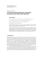
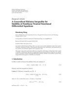
Figure 1: When τ h 0.05, the wave graph of u at various times.
Let x
L
−20, x
R
20, T 1.0, and υ γ 1. Since we do not know the exact solution of
1.4-1.5, an error estimates method in 21 is used: a comparison between the numerical
solutions on a coarse mesh and those on a refine mesh is made. We consider the solution on
mesh τ h 1/160 as the reference solution. In Table 1,wegivetheratiosinthesenseofl
∞
at various time steps.
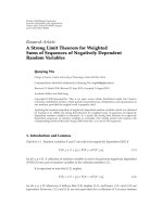
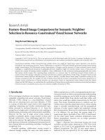
When τ h 0.05, a wave figure comparison of u and ρ at various time steps is as in
Figures 1 and 2.
From Table 1, it is easy to find that the difference scheme in this paper is second-order
convergent. Figures 1 and 2 show that the height of wave crest is more and more low with
time elapsing due to the effect of damping and dissipativeness . It simulates that the continue
energy Et of problem 1.4–1.7 in Lemma 1.1 is digressive. Numerical experiments show
that the finite difference scheme is efficient.
Boundary Value Problems 15
−0.2
0
0.2
0.4
0.6
0.8
1
1.2
1.4
1.6
1.8
t = 0
t = 0.5
t = 1
−20 −15 −10 −5
0 5 10 15 20
Figure 2: When τ h 0.05, the wave graph of ρ at various times.
Acknowledgments
The work of Jinsong Hu was supported by the research fund of key disciplinary of application
mathematics of Xihua University Grant no. XZD0910-09-1. The work of Youcai Xu was
supported by the Youth Research Foundation of Sichuan University no. 2009SCU11113.
References
1 C. E. Seyler and D. L. Fenstermacher, “A symmetric regularized-long-wave equation,” Physics of
Fluids, vol. 27, no. 1, pp. 4–7, 1984.
2 J. Albert, “On the decay of solutions of the generalized Benjamin-Bona-Mahony equations,” Journal of
Mathematical Analysis and Applications, vol. 141, no. 2, pp. 527–537, 1989.
3 C. J. Amick, J. L. Bona, and M. E. Schonbek, “Decay of solutions of some nonlinear wave equations,”
Journal of Differential Equations, vol. 81, no. 1, pp. 1–49, 1989.
4 T. Ogino and S. Takeda, “Computer simulation and analysis for the spherical and cylindrical ion-
acoustic solitons,” Journal of the Physical Society of J apan , vol. 41, no. 1, pp. 257–264, 1976.
5 V. G. Makhankov, “Dynamics of classical solitons in non-integrable systems,” Physics Reports. Section
C, vol. 35, no. 1, pp. 1–128, 1978.
6 P. A. Clarkson, “New similarity reductions and Painlev
´
e analysis for the symmetric regularised long
wave and modified Benjamin-Bona-Mahoney equations,” Journal of Physics A, vol. 22, no. 18, pp. 3821–
3848, 1989.
7 I. L. Bogolubsky, “Some examples of inelastic soliton interaction,” Computer Physics Communications,
vol. 13, no. 3, pp. 149–155, 1977.
8 B. Guo, “The spectral method for symmetric regularized wave equations,” Journal of Computational
Mathematics, vol. 5, no. 4, pp. 297–306, 1987.
9 J. D. Zheng, R. F. Zhang, and B. Y. Guo, “The Fourier pseudo-spectral method for the SRLW equation,”
Applied Mathematics and Mechanics, vol. 10, no. 9, pp. 801–810, 1989.
10 J. D. Zheng, “Pseudospectral collocation methods for the generalized SRLW equations,” Mathematica
Numerica Sinica, vol. 11, no. 1, pp. 64–72, 1989.
16 Boundary Value Problems
11 Y. D. Shang and B. Guo, “Legendre and Chebyshev pseudospectral methods for the generalized
symmetric regularized long wave equations,” Acta Mathematicae Applicatae Sinica,vol.26,no.4,pp.
590–604, 2003.
12 Y. Bai and L. M. Zhang, “A conservative finite difference scheme for symmetric regularized long wave
equations,” Acta Mathematicae Applicatae Sinica, vol. 30, no. 2, pp. 248–255, 2007.
13 T. Wang, L. Zhang, and F. Chen, “Conservative schemes for the symmetric regularized long wave
equations,” Applied Mathematics and Computation, vol. 190, no. 2, pp. 1063–1080, 2007.
14 T. C. Wang and L. M. Zhang, “Pseudo-compact conservative finite difference approximate solution
for the symmetric regularized long wave equation,” Acta Mathematica Scientia. Series A, vol. 26, no. 7,
pp. 1039–1046, 2006.
15 T. C. Wang, L. M. Zhang, and F. Q. Chen, “Pseudo-compact conservative finite difference approximate
solutions for symmetric regularized-long-wave equations,” Chinese Journal of Engineering Mathematics ,
vol. 25, no. 1, pp. 169–172, 2008.
16 Y. Shang, B. Guo, and S. Fang, “Long time behavior of the dissipative generalized symmetric
regularized long wave equations,” Journal of Partial Differential Equations, vol. 15, no. 1, pp. 35–45,
2002.
17 Y. D. Shang and B. Guo, “Global attractors for a periodic initial value problem for dissipative
generalized symmetric regularized long wave equations,” Acta Mathematica Scientia. Series A, vol.
23, no. 6, pp. 745–757, 2003.
18 B. Guo and Y. Shang, “Approximate inertial manifolds to the generalized symmetric regularized long
wave equations with damping term,” Acta Mathematicae Applicatae Sinica, vol. 19, no. 2, pp. 191–204,
2003.
19 Y. Shang and B. Guo, “Exponential attractor for the generalized symmetric regularized long wave
equation with damping term,” Applied Mathematics and Mechanics, vol. 26, no. 3, pp. 259–266, 2005.
20 F. Shaomei, G. Boling, and Q. Hua, “The existence of global attractors for a system of multi-
dimensional symmetric regularized wave equations,” Communications in Nonlinear Science and
Numerical Simulation, vol. 14, no. 1, pp. 61–68, 2009.
21 B. Hu, Y. Xu, and J. Hu, “Crank-Nicolson finite difference scheme for the Rosenau-Burgers equation,”
Applied Mathematics and Computation, vol. 204, no. 1, pp. 311–316, 2008.