báo cáo hóa học:" Research Article A Formal Model for Performance and Energy Evaluation of Embedded Systems" pot

Hindawi Publishing Corporation
EURASIP Journal on Embedded Systems
Volume 2011, Article ID 316510, 12 pages
doi:10.1155/2011/316510

Research Article
A Formal Model for Performance and Energy Evaluation of
Embedded Systems
Bruno Nogueira,1, 2 Paulo Maciel,1 Eduardo Tavares,1 Ermeson Andrade,1 Ricardo Massa,1
Gustavo Callou,1 and Rodolfo Ferraz1
1

Informatics Center, Federal University of Pernambuco, 50.740-560 Recife, Brazil
Unit of Garanhuns, Federal Rural University of Pernambuco, 55.296-901 Garanhuns, Brazil

2 Academic

Correspondence should be addressed to Bruno Nogueira,
Received 2 June 2010; Accepted 21 September 2010
Academic Editor: Dietmar Bruckner
Copyright © 2011 Bruno Nogueira et al. This is an open access article distributed under the Creative Commons Attribution
License, which permits unrestricted use, distribution, and reproduction in any medium, provided the original work is properly
cited.
Embedded systems designers need to verify their design choices to find the proper platform and software that satisfy a given set of
requirements. In this context, it is essential to adopt formal-based techniques to evaluate the impact of design choices on system
requirements. To be useful, such techniques must produce accurate results with minimal computation time. This paper proposes
an approach based on Coloured Petri Nets for evaluating embedded systems performance and energy consumption. In particular,
this work presents a method for specifying and evaluating the workload and the platform components, such as processors and
shared or private memories. The method is applied to model single processor and multiprocessor platforms. Experimental results
demonstrate an average accuracy of 96% in comparison with the respective measures assessed from the real hardware platform.

1. Introduction
The design of embedded systems usually must take into
account several nonfunctional constraints, such as performance, size, weight, cost, reliability, and durability. The rapid
growth of embedded systems in new application domains
introduces new restrictions, which in turn raises new
research and technical challenges. One prominent research
area is related to battery-operated devices, in which energy
consumption plays an important role. The low-power design
has grown in importance with the proliferation of such
devices. The main challenge is to reduce energy consumption
without jeopardizing the performance requirements.
Modern embedded systems are composed of a set of
interconnected processing, communication, and storage
elements. Very often, these elements are integrated into
a single circuit (System-on-Chip). Software (instructions
streams/workload) executing on the processing elements
drives the behavior of the system. In contrast to a desktop
system, which executes a variety of workloads, normally

embedded systems execute only one workload, repeatedly.
The characteristics of the workload and the processing elements dictate the usage of communication and storage elements. In turn, the characteristics of the communication and
storage elements influence the rate at which the workload is
executed. Therefore, energy consumption and performance
are a function of the characteristics of the workload and the
architectural elements, and thus, estimating these metrics is
not an ordinary task.
Given the wide range of platform options and software
optimizations, designers need to verify their design choices
to find the proper platform and software that satisfy a given
set of requirements. Measurement of the actual performance

and energy consumption characteristics on real hardware is
often not feasible, since this would require the construction
of a large number of hardware prototypes. In this context,
many model-based approaches for estimating energy consumption and performance have been developed over the
last years (e.g., [1–4]). Some of these model the energy
consumption adopting cycle-level simulators (also known as


2
architecture level model approach) [2, 5]. Despite providing
very accurate estimates, the low abstraction level adopted by
current approaches demands an enormous computational
effort, which restricts the applicability for large codes.
This work presents a discrete event modeling strategy,
based on Coloured Petri Net formalism (CPN) [6], for
performance and energy consumption evaluation of embedded systems using the architecture level model approach. In
particular, this paper presents a novel method for specifying
and evaluating the performance and energy consumption
of embedded systems considering different configurations
for workload and the platform components, such as processors and memories. The method is applied to model
a real platform, namely, NXP LPC2106, and a theoretical
multiprocessor platform. The high level of abstraction of
the proposed models allows for fast but accurate estimates.
Additionally, although specific platforms have been considered, the modeling approach can be easily applied to other
architectures.
Petri Nets (PNs) [7] are well suited to model computer
architectures, since both parallelism and conflict, two important characteristics present in modern computer systems, are
easily modeled using this formalism. Besides, PN extensions,
such as CPN, have proven to be a powerful technique to
evaluate performance indices in computer systems [8].

This paper is organized as follows. Section 2 presents
related work. Section 3 introduces the required concepts for
a better understating of this work. Section 4 presents the
proposed approach. Section 5 presents some experiments
and Section 6 concludes the paper.

2. Related Work
Many approaches have been conceived to model energy
consumption in embedded systems. However, few consider
multiprocessor architectures. The approaches can be generally classified into two main categories: (i) architecture level
(or hardware level) models and (ii) instruction level models.
Architecture level models calculate power and energy from
detailed descriptions that may comprise circuit level, gate
level, and register transfer (RT) level. Instruction level
models deal only with instructions and functional units from
the software point of view and without knowledge of the
underlying hardware organization [9].
The first energy instruction model was introduced in
[1, 10]. These works assign an energy cost to each instruction
(or sequence of instructions). The cost per instruction is
assessed by measuring the average current of the processor
when it executes that instruction. Interinstruction effects are
also considered. However, the time required to characterize
an architecture is a great issue, since the number of measurements grows exponentially with the number of instructions
in the Instruction Set Architecture (ISA).
Oliveira et al. [11] proposed a simulation approach based
on Coloured Petri Net. That work proposed a stochastic
model for the 8051 microcontroller instruction set. The
method adopted CPN to model the control flow of a given
application and assigned probabilities to conditional branch

EURASIP Journal on Embedded Systems
instructions, which were translated to CPN transition guard
expressions. The main drawback of that strategy is the model
complexity, which grows with the application size, hence
causing considerable negative impact on simulation time.
Such an approach does not allow the evaluation of real-life
complex applications or even reasonable size programs. That
method was extended in [3] to simplify the model. Although
the simulation time is significantly reduced, it is still heavily
affected by the code size.
Another instruction level approach, known as functional-level power analysis (FLPA), was introduced in [12] and
further extended in [4]. In this method, the processor is
separated into functional blocks (such as fetch unit, processing unit, and internal memory). The power consumption
of each block is characterized through mathematical functions obtained from several measurements and/or simulations. Thus, the power consumption is obtained by adding
up the consumption of all blocks. Although being very fast
and having relative good accuracy for estimating power
consumption, the proposed analytical modeling presents
some limitations for estimating execution time, which in
turn affects the energy consumption estimation as shown in
their experimental results [4].
Since existing approaches work at a very low level of
abstraction (e.g., [2, 5]), architecture level models are known
to be very time consuming. Besides, those approaches also
need a low-level representation (such as RTL level) of the
architecture to allow the power characterization. However,
these details of implementation are rarely available for most
commercial processors.

3. Modeling Formalisms

A stochastic discrete event system (SDES) [13] is a system
which occupies a single state for some duration of time,
after which an atomic event causes an instantaneous state
transition to occur. They are called discrete event systems
because their state does not change between subsequent
events, whereas state changes occur continuously in a continuous event system. In SDES, stochastic delays (described by
probability distribution functions) and probabilistic choices
[13] are used to model uncertainties in the system, which
may be introduced by many factors such as unpredictable
human actions and machine failures. Many SDES models
have been developed, for instance, stochastic automata,
queuing models, and stochastic Petri nets. In this work,
Coloured Petri Nets (CPNs) and Discrete Time Markov
Chains (DTMCs) are adopted to model, respectively, the
platform and the workload. A comprehensive overview of
the modeling possibilities with SDES is out of scope for
this paper, but basic concepts are sketched. A much more
thorough description of SDES is available in [13–15].
3.1. Discrete Time Markov Chains. A Discrete Time Markov
Chain {Xt } can be defined as a sequence of random variables
X0 , X1 , X2 , . . . , Xk in which each one of them takes a discrete
number of possible values, and where t is defined over a
discrete set. The value taken by Xt is referred to as the state


EURASIP Journal on Embedded Systems

3

of the DTMC at time t. Following the Markov property, at

any t = 0, 1, 2, ..., k the conditional probability distribution
of the random variable Xk given the values of its predecessors
X0 , X1 , . . . , Xk−1 depends only on the value of its immediate
predecessor Xk−1 but not on the values of X0 , X1 , . . . , Xk−2 .
Thus, this property states that
Pr(Xk = xk | X0 = x0 , X1 = x1 , . . . , Xk−1 = xk−1 )
= Pr(Xk = xk | Xk−1 = xk−1 ).

(1)

A DTMC is said to be time homogeneous, if Pr(Xk+1 =
j | Xk = i) is independent of k. In this work, we consider
only time homogeneous DTMCs.
Associated with a DTMC is a matrix called the one-step
probability transition matrix, denoted by P, whose (i; j)th
element is given by the probability pi j of a state transition
from state Xk = i to Xk+1 = j in a single step (pi j = Pr[Xk+1 =
j | Xk = i]):
⎛

⎞
p11 p12 · · · p1n
⎜
⎟
⎜p
⎟
⎜ 21 p22 · · · p2n ⎟
⎜
⎟
P=⎜ .

. ..
. ⎟,
⎜ .
.
. ⎟
⎜ .
. . ⎟
.
⎝
⎠
pn1 pn2 · · · pnn

0 ≤ pi j ≤ 1,

n
j =1

(2)

pi j = 1 for each i.

DTMCs can be represented by a directed graph, known
as the state-transition diagram. The nodes represent the
states of the DTMC and the edges, the transitions between
the states labeled by the respective one-step transition
probabilities.
The main purpose of establishing a DTMC and the
corresponding probability transition matrix P is to obtain
the probability for the modeled system to be in a particular
state. From the state probabilities, several performance

metrics can be obtained. Let π = (π1 , π2 , π3 , . . . , πn ) be the
unique vector such that π = πP and n=1 πk = 1 with
k
πk ≥ 0. If the DTMC is finite and irreducible, such unique
π exists and is called stationary probability vector [16]. More
specifically, πi is proportion of time spent in state i in the
long-run. Moreover, it can be shown that the average number
of visits v j to state j between occurrences of state i is given by
vj =

πj
.
πi

(3)

To evaluate DTMC models, the SHARPE tool [17] has
been adopted by this work.
3.2. Coloured Petri Nets. A CPN [6] is a bipartite-directed
graph, consisting of two types of vertices: (i) places (drawn as
circles) and (ii) transitions (drawn as bars). Places model the
states, and transitions represent the events of the system. In
CPN, a transition is able to fire (enabled) when (i) it has one
token of the proper type on each of its input arcs, and (ii) the
guard (Boolean expression) attached to the transition holds.

An enabled transition can fire and thus remove tokens from
its input places and generate tokens for its output places.
The concept of hierarchical design is supported by CPN.
The basic idea is to allow the construction of a large model

by using a number of smaller models. These small models
are called pages and are connected to each other by places
called ports. Such places can be input or output types. It is
also possible to use time in CPN models. Time is handled
by introducing a global clock and allowing each token to
carry a time stamp. A token cannot be used unless the value
of the clock has passed or is equal to the value of the time
stamp. Intuitively, each time stamp indicates the earliest time
at which the token may be used.
In order to show some concepts of CPN, a very simple
model is depicted in Figure 1(a) which models the first two
stages of a generic pipelined processor. The CPN model
consists of two components: pipeline flow and pipeline
controller. The places start, fetching, fd, decoding, and execute
model the states of the instruction in the pipeline flow.
The place control models the control of the flow of instructions through the pipeline. Attached to the transitions f2 and
d2, there is a delay of 1, which means one clock cycle, that is,
the time required to fetch and decode an instruction in this
processor. The marking of places start and fetching consists of
one token each, both with value (colour) undefined and time
stamp 0, meaning that there is one instruction being fetched
and the other is waiting to be fetched. Since these instructions
have not been decoded yet, they are classified as undefined
in the model. As can be seen in Figure 1(a), transition f2 is
enabled because there is a token of type INSTRUCTION in
its input place (fetching), and transition f1 is disabled because
there is no token of colour fetch in the place control. Similar
concepts apply to the other disabled transitions.
When the transition f2 is fired (see Figure 1(b)), a token
is removed from place fetching and two tokens are created in

places control and fd. The new tokens get a time stamp which
is the current time plus one. At this moment, transition f1 is
enabled as well as transition d1. The simulation continues
as long as enabled transitions can be found. As can be
seen, the model structure makes it impossible for two
instructions occupy the places fetching or decoding at the
same time. Additionally, the function dec() in the arc (d2,
execute) generates instructions and puts them to execute.
This function will be explained in more details in Section 4.1.
To assist our modeling we use the tool CPN Tools [18],
which is a mature and well-tested tool that supports editing,
simulation, and analysis of CPN.

4. Modeling Approach
In this section, the proposed method is presented and applied
to evaluating software applications running on the NXP
LPC2106, an ARM7TDMI-S-based architecture [19].
4.1. Architecture Modeling. The LPC2106 has 128 kB of
on-chip FLASH and 64 kB of on-chip SRAM. It has an
ARM7TDMI-S processor which enables system designers to
build embedded devices requiring small size, low power,


4

EURASIP Journal on Embedded Systems

1`undefined@0
i
start

1
INSTRUCTION

INSTRUCTION
1`undefined@0
fetching 1

i

f1

1`fetch

i

1`fetch

INSTRUCTION

1`undefined@0
i
start

@+1
f2

1

control

PIPELINE

1`decode
execute

dec()

INSTRUCTION

d2
@+1

i

fd
INSTRUCTION
i
1`decode
i

decoding
INSTRUCTION

i
1`undefined@1

control
PIPELINE

1`decode

execute

d1

1`fetch

1`fetch@1+++
1`decode@0
2

Clock: 1

dec()

INSTRUCTION

d2
@+1

(a)

@+1
f2

i

fetching

1`fetch

i

1`decode@0
Clock: 0

i

f1

1
INSTRUCTION

i

1 fd
INSTRUCTION
i
1`decode
i

decoding

d1

INSTRUCTION
(b)

Figure 1: CPN model for the first two stages of a pipelined processor.

INSTRUCTION

EXECUTE

execute

EXECUTE

PIPELINE

r2

control

MEMORY

1`execute++1`decode++1`fetch
c2
CACHE
FLASH MEMORY
FLASH MEMORY

FETCH/DECODE
FETCHDECODE

CACHE

RAM MEMORY
RAM MEMORY

r1

MEMORY

c1
3`undef
start
INSTRUCTION

Figure 2: CPN model for the LPC2106 architecture (High-level view).

and high performance. Such processor is a 32-bit RISC
architecture that consists of a program control unit, an
address generator, an integer data path, a general-purpose
register bank, and a 3-stage pipeline. An important characteristic of the LPC2106 is an instruction prefetch module,
known as Memory Accelerator Module (MAM). The MAM
is connected to the local bus and is placed between the
FLASH memory and the ARM7TDMI-S core. Like a cache,
the MAM attempts prefetch the next instruction from the
FLASH memory in time to prevent CPU fetch stalls.
In order to model the LPC2106 architecture, a library
of generic blocks of CPN models has been constructed.
These blocks can be combined in a bottom-up manner
to model sophisticated behaviors. Modeling a complex
architecture thus becomes a relatively simple process. The
proposed CPN models are high-level representations that
focus on what the architecture should perform instead of on
how it is implemented. Moreover, it is important to stress

that once constructed, a building block can be reused in other
platform models.
Figure 2 presents the highest-level view of the model,

which is composed of the following building blocks (pages,
see Section 3.2): flash memory, ram memory, fetch/decode,
and execute. The fetch/decode and execute blocks model,
respectively, the first two and the last stages of the LPC2106’s
pipeline. Between these two blocks, there is a place (control),
which controls the flow of instructions through the pipeline
(see Figure 1). The marking of place control represents the set
of available functional units. The ram memory block models
the SRAM memory, and the flash memory block, the FLASH
memory. In these models, timing information is expressed in
cycles and is represented through transition firing delays. The
energy consumption is expressed in nJ units and is modeled
through the addEnergy function, which adds the specified
energy consumption to the global simulated consumption.
Information regarding time and energy consumption was


EURASIP Journal on Embedded Systems

5

if c = false
then
1`i++3`bubble
else
1`i
f2

c

fetching
In
@+1
i
f1

mamaccess()

i

End
flash

[c=true]
Cache hit

CACHE

Cache miss

c

flash
Out
CACHE

[c = false]

CACHE

c

action
(addEnergy(0.27));

c2
Out

Flash connection

start
In

CACHE
c
c1
In
@+3

c

i

INSTRUCTION
(a) Fetch/decode building block

(b) FLASH memory building block

Figure 3: Fetch stage and FLASH memory connection.

INSTRUCTION
executing1

i

i

i
[#t i<> mul andalso
#t i<> bubble]
@+1
[#t i=mul]
@+3

mul action
(addEnergy(3∗ 1.3));
i

alu
i

action
(addEnergy(1.54));

@ + 1 nop action
(addEnergy(1.26));

executing2

i

[#shift i=true]

[#shift i=false]
Not shift

i

[#t i=bubble]

@ + 1 Shift action
(addEnergy(1.32));
INSTRUCTION
executing3

i

Figure 4: Excerpt of the execute building block.

assessed through measurements using the AMALGHMA
platform (see Section 4.4) as well as from LPC2106 datasheet
[20] and ARM7TDMI-S reference manual [19].
Except for two differences, the fetch/decode block is equal
to the model presented in Figure 1. Since, in LPC2106
architecture, the FLASH memory stores the application
code, the first difference is that the fetch stage is now
connected to the flash memory block. Figure 3(a) shows this
connection and Figure 3(b) shows the flash memory block.
If the data to be fetched is available in the MAM latches
(c = true), no flash access is required. Otherwise (c = false)
one flash access is required and, thus, the respective energy

consumption must be computed. The function mamaccess

returns a Boolean value. Given the hit ratio of the application
under evaluation, firstly it generates a random number with
uniform distribution between 0 and 1 and then compares
it to the MAM hit ratio. If the random number is less or
equal to the hit ratio, this function returns true, or false,
otherwise. Accesses to the FLASH memory stall the pipeline,
causing the introduction of pipeline bubbles in the wake of
the stalled instruction (see the output arc of transition f2).
The bubbles pass through all stages of the pipeline like any
other instruction and then are discarded in the last pipeline
stage. The MAM miss ratio must be provided to define the
evaluation scenario. To obtain this information, a simple
trace-driven simulator was implemented for supporting the


6

EURASIP Journal on Embedded Systems

estimation of miss ratios related to specific instruction
patterns. This simulator receives as input a trace of the
executed instruction addresses and reports the estimated
MAM miss ratio.
The second difference is that there are additional transitions in the fetch/decode block that are responsible for
exchanging the instructions in the fetch and decode stages
for bubbles. These transitions become enabled when place
control receives a token with colour flush, generated by the
execute block when it simulates a branch instruction.

The LPC2106 instruction set has been divided into five
classes of instructions according to their performance and
energy consumption characteristics: load, store, conditional
branch, unconditional branch, data operations, and multiply. For each instruction class, the execute block defines
the next states and what should be done on the way from
one state to another. Figure 4 shows an excerpt of the
execute block. As can be seen, depending on its class, the
instruction may take one of the paths described in the
model and the correspondent delay and energy consumption
computed. At decode stage, dec function (see Figure 1)
classifies instructions into one of the instructions classes.
This function returns a value of type INSTRUCTION in a
probabilistic way, such that if an instruction of class c1 is
executed with a frequency of 50% in the code to be evaluated,
this function will return an INSTRUCTION value of class c1
with probability of 50%.
4.2. Workload Specification. As stated earlier, the dec function
generates instructions according to the frequency in which
each instruction class is executed in the application under
evaluation. Since this frequency distribution is dependent on
a given software and input data, we devised a method for
capturing this information. The method consists in mapping
the application code (with annotations) into a DTMC. More
specifically, the Control Flow Graph (CFG) of the application
is mapped into an irreducible DTMC.
Each basic block Bi in the CFG is mapped into a state
Xi in the DTMC. Similarly, control flow edges are mapped
as transitions between states and are labeled by the state
transition probabilities, as
P Bi , B j = Pr Bi jumps to B j ,

(4)

which defines the probability of executing B j after Bi .
Such probabilities are obtained from annotations in the
application code.
Figure 5(a) shows an example of code, in which annotations are comments. In this example, the annotation at line 4
indicates that the expression x < 10 evaluates to true with a
probability of 50%. The annotation at line 6 indicates that
the iterative structure is executed 9 times. The values for
the annotations may be captured, for instance, from (i) ad
hoc designer knowledge, (ii) a more abstract system model,
and/or (iii) extensive profiling. Several execution scenarios
can be evaluated by simply changing these values. Figure 5(b)
depicts the resulting DTMC, where the reader should note
an additional transition from state 5 to state 1 (i.e., from the

final to the starting point of the application), which is added
to make the DTMC irreducible.
The objective in such a mapping is to compute the average number of times each basic block in the CFG executs
(visiting number). Given the stationary probability vector
π = (π1 , π2 , . . . , πk ) of the mapped DTMC, which is obtained
numerically by the SHARPE tool, let v = (v1 , v2 , . . . , vk ) be
the vector with the average number of executions of each
basic block B1 , B2 , . . . , Bk , where Bk contains the ending point
of the application. Then, v is determined by (see (3))
v=

π
π1 π2

, ,..., k .
πk πk
πk

(5)

Given the average number each basic block executs, the
frequency in which each instruction is executed can be
obtained, and hence the execution frequency of each class.
The methodology flow for the estimation of the energy
consumption and execution time in an architecture for
a given application is shown in Figure 6. The architectural
model is constructed by the composition of CPN building
blocks (right side of Figure 6). The building blocks represent
functional units of the architecture under evaluation and
are modeled in a high abstraction level, allowing flexibility,
reuse, and rapid evaluation. These building blocks are annotated with values regarding energy consumption (addEnergy
function) and performance (CPN delays) of the modeled
functional unit. Next, the code which will execute on the
embedded platform is mapped on the architectural model by
a compiler (see Section 4.5). Finally, the model evaluation is
made by means of stochastic simulation (Section 4.3).
4.3. Evaluation. The evaluation is made by means of simulation. The facilites of CPN Tools have been adopted to
define analysis functions and to perform data collection.
Basically, two performance metrics were defined: (i) the
average execution time per instruction and (ii) the average
energy consumption per instruction. Given these metrics
and the number of executed instructions in the application and the processor’s operating frequency, the overall
energy consumption and execution time of an application is
obtained.

Firstly, a breakpoint monitor [8] was defined and assigned
to the last transition in the execute block. This transition
is always fired by all instruction classes. The breakpoint
monitor collects data and tests if the metrics satisfy the
stop criterion. If so, the simulation stops; otherwise, the
simulation continues. To calculate the metrics, two data
are collected on the firing of the transition linked with the
breakpoint monitor: (i) the interval firing time, that is, the
current time minus the last firing time, and (ii) the interval
energy consumption, that is, the current global energy
consumption minus the global energy consumption of the
last firing. We designed a set of statistical functions so that a
confidence interval for the metrics could be constructed. The
stop criterion defines that if the confidence interval of these
two metrics satisfies the specified precision, the simulation
stops. The precision is specified by two parameters: (i) the
confidence level and (ii) the relative error. This work adopted


EURASIP Journal on Embedded Systems

7

Table 1: Experimental results.

adpcm
bcnt
binary search
bubble sort
convolution

fdct
oximeter (1)
oximeter (2)
oximeter (3)

Estimated
12397.3
55.2
5.9
6162.3
964.9
90.9
11.6
11.7
3357.2

Execution Time (μs)
Measured
13080.1
56.1
5.8
6138.3
1076.9
93.4
11.9
12.3
3379

Error
5.22%

1.60%
1.72%
0.39%
10.2%
2.68%
2.52%
5.26%
0.65%

(1) int main() {
int x, y
(2)
(3)
if (x < 10) // <0.5>
(4)
{
(5)
for (y = 0; y < 9; y++) { //<9>
(6)
x++;
(7)
}
(8)
} else { // <0.5>
(9)
x = 0;
(10)
}
(11)
(12)

(13) }

Estimated
1065.77
4.62
0.49
5189.8
76.9
7.83
0.99
0.99
283.05

1

Energy Consumption (μJ)
Measured
1097.28
4.63
0.50
5247.6
80.1
8.21
1.01
1.07
257.21

0.5

0.5

2
1

4

0.9

0.1

3

1
5

(a) Code with annotations

(b) Mapped DTMC

Figure 5: Code mapping example.

Memory 1
Annotated
source code

Protocol 1

Processor 2

Cache 1

Processor 1
Transforming
code → DTMC

Memory 2

DTMC
Component
composing

DTMC
evaluation

#inst. count
#Inst. freq.

Mapping the
workload
into the
architecture
model

Architecture
model

Evaluation

Figure 6: Proposed methodology flow.

1

Error
2.87%
0.22%
2%
1.10%
4%
4.63%
1.98%
7.48%
10.02%


8

EURASIP Journal on Embedded Systems
Agilent
DSO03202A

Philips
LPC2106
Channel 1

1
(1) void BubbleSort (int Array[])
2
(2) {
3
int i, j;
(3)

4
int k = NUMELEMENS-1;
(4)
5
(5)
6
for (I = 0; i < NUMELEMENS; i++)
(6)
{
7
(7)
8
for (j = 0; j(8)
9
{
(9)
10
if (Array[j] > Array[j + 1])
(10)
{
11
(11)
12
swap(Array, j, j + 1);
(12)
}
13
(13)
14

}
(14)
(15)
k−−;
15
(16)
}
16
(17) }
17

CPU
I/O Port
GND

Channel 2

1 Ohm

Serial communication

// <100>
// <4950>
// <0.5>

PC with AMALGHMA

Figure 9: Bubblesort algorithm.

Figure 7: Measurement scheme.

Energy consumption (µJ)

Figure 8: Code optimizations.

0.8

0.81

0.82

0.83

0.84

0.85

0.86

MAM hit ratio

Figure 10: Bubblesort: energy consumption in function of the
MAM hit rate variations.

Table 2: Simulation time comparison.
A1 (s)
2
2
1085

0.87

0

Measured
Estimated

Task 1
Task 2
Task 3

1000
0.88

Inlining

2000

0.89

8 level
unrolling

3000

0.9

3 level
unrolling

4000

0.91

2 level
unrolling

5000

0.92

Original

6000

0.934339

1613.5 1469.1

Energy consumption (µJ)

7000

5247.6 5189.8
4872.2 4847 4808.5 4554 4609.8
4396.9

A2 (s)
4
3
2

a confidence level of 95% and a maximum relative error of
2%.
4.4. Measuring Strategy. This section describes the measuring method adopted to obtain the energy consumption and
execution time values employed in the proposed models. To
capture the average energy consumption of each functional
unit defined in the model, assembly codes that stimulate,
separately, the respective functional unit of the LPC2106
have been implemented, uploaded on the platform, executed,
measured, and then the obtained data were statistically
analyzed. For example, to capture the average power consumption when a MAM miss occurs, an assembly code that
forces MAM misses was designed.

The AMALGHMA (Advanced Measurement Algorithms
for Hardware Architectures) tool has been implemented for
automating the measuring activities. AMALGHMA adopts a
set of statistical methods, such as bootstrap and parametric
methods, which are important in the measurement process
due to several factors, for instance, (i) oscilloscope resolution and (ii) resistor error. Besides, the results estimated
by AMALGHMA were compared and validated considering LPC2106 datasheet as well as ARM7TDMI-S reference
manual.
The measurement scheme is shown in Figure 7. To measure power consumption, a workstation executing the
AMALGHMA tool is connected to an Agilent DSO03202A
oscilloscope, which captures the platform-drained current by
measuring the voltage drop across a 1 Ohm sense resistor
(average microcontroller impedance is order of magnitude higher than this). The oscilloscope is also connected
to an I/O port of the LPC2106, which is used to monitor
the code’s starting and end times. Given this, the code’s
execution time is also estimated. Even for very short duration
software functions, the AMALGHMA tool is able to estimate

EURASIP Journal on Embedded Systems

9

Microcontroller 1
(LPC2106)

Microcontroller 2
(LPC2106)

Data

Data

Code

PROC 1
Proc

Code
e1

[]

e2
MEMORY

EXT MEM

EXTMEMORY

EXT MEM

External
memory

PROC 2
Proc

(a) Multiprocessor environment

(b) Multiprocessor CPN model

Figure 11: Multiprocessor case study.

DECLARATIONS
colset MEMORY = with read | write
timed;
colset EXTMEMORY = list MEMORY
timed;

EXTMEMORY
ext1
In
[check(I, read)]
@+2
action
(addEnergy(3));

rmread(I)

I

rm write I

fun rmread (x::l) = if x = read then
rmread (l) else x::l |
rmread ([]) = [];

I
[check(I, write)]
write
mem

read
mem
getread(I)

Out
ext2
MEMORY

@+2
action
(addEnergy(3.5));
1`write

(a)

fun getread (x::l) = if x = read then
read::getread (l) else [] |
getread ([]) = [];
fun check (x::l, t) = if x = t then true
else false |
check ([],t) = false
(b)

Figure 12: External memory model.

the average execution time, its energy consumption, and
other related statistics. For doing that, sampling and statistics
strategies have been implemented [21].
4.5. PECES Tool. An additional contribution of this work
was the development of a computational tool to automate
same steps of the proposed methodology. The tool was
named PECES (Performance and Energy Consumption
Evaluation of Embedded Systems). It receives the annotated
source code and the architecture model as input and returns
the average execution time and energy consumption as
output.
The following steps are performed by PECES to evaluate
a code.
(1) It compiles the application source code using the
option to generate intermediate assembly code. GCC
(arm-uclibc-gcc [22]) has been adopted as compiler.
(2) PECES builds the Control Flow Graph (CFG) using
the intermediate code generated in the previous step.

(3) It uses the CFG and the annotations from the source
code to generate the corresponding irreducible
DTMC.
(4) The DTMC is numerically evaluated in SHARPE, so
as to obtain the stationary probabilities.
(5) It uses the stationary probabilities to calculate the
average number of execution for each basic block
and, then, the number of times each instruction is
executed. Next, PECES clusters instructions from the
same class and calculates the frequency each class
executs.
(6) The distribution frequency is written in the architecture model.
(7) PECES invokes Access/CPN tool [23] to simulate the
architecture model.
(8) Finally, the tool uses the average execution time
per instruction and the average energy consumption
per instruction obtained from the previous step to
calculate the average execution time and the energy
consumption.


10

5. Experimental Results
This work has conducted some case studies to evaluate the
proposed estimation methods. The case studies consist of (i)
Motorola’s Powerstone benchmark suite codes (adpcm, bcnt,
and fdct), (ii) common search/ordering/signal processing
algorithms (binarysearch, bubblesort, and convolution), (iii)
a customized example, and (iv) a real-world biomedical

application (a pulse oximeter). The pulse oximeter case study
is composed of three concurrent tasks; hence it has been
divided into three separate experiments. All experiments
were performed on an Intel Core 2 Duo 1.67 GHz, 2 Gb
RAM, and Windows Vista OS.
Table 1 shows the estimated energy consumption and
execution time compared to the measured values for the case
studies. The comparison yields an average error of 3.36% and
maximum error of 10.2% for the estimated execution time.
Regarding the energy consumption, the average error was of
3.81% with maximum of 10.02%.
The pulse oximeter experiment was adopted to compare
the simulation time of the proposed approach against
the instruction-simulation method presented in [3], which
also modeled the LPC2106 (although the MAM has not
been considered) and reported an average error of 4% for
the estimated metrics. Table 2 depicts quantitative results,
in which A2 represents the proposed approach, and A1
represents the approach presented in [3]. Results in A2 also
include the time to generate and evaluate the DTMCs, which
took less than one second for all codes. Results show that
the simulation time in both methods are almost the same,
except for the third task. In this task, the proposed approach
was 542 times faster. The huge difference is mainly because
[3] simulates the control flow of the application; hence, the
simulation model and the simulation time grow with the
code size. On the other hand, in the method proposed by this
work, the model has a fixed size; the variations occur only on
the frequency in which each instruction class is executed.

5.1. Applications of the Method. Code optimizations, such
as loop unrolling and function inlining, have proven to be
successful techniques to improve the system performance.
A very useful application for the proposed method is to
verify the effect of these common code optimizations on
system energy consumption. The bubblesort experiment has
been used to demonstrate how such what-if analysis may be
carried out.
The bubblesort code was optimized in four steps.
From step to step more aggressive optimizations have been
included. Figure 8 shows the results of this experiment.
It can be seen that by applying such optimizations the
energy consumption was optimized in 225%. The average
error for the estimated values was of 4.38%, showing that
the proposed method may be successfully employed for
performing energy aware code optimizations.
The proposed method is also useful when it comes
to evaluating code operation scenarios, such as best-case,
average-case, and worst-case scenarios. The bubblesort code
has been used to evaluate such application.

EURASIP Journal on Embedded Systems
The bubblesort code is depicted in Figure 9, where the
reader should note that all code flow variance is defined
by the three structures at lines 6, 8, and 10. The iteration
number at lines 6 and 8 is array-length dependent, in
which a deterministic behavior is performed. On the other
hand, the control structure at line 10 has a probabilistic
behavior, depending on the ordering level of the array. In the
worst-case scenario, the array is fully unordered; hence the

function swap will be called every time. Such scenario may be
evaluated by setting the annotation value at line 10 to 1. The
best-case scenario happens when the array is fully ordered.
In this case, the function swap will never be called. By simply
setting the annotation value at line 10 to 0, this scenario may
be evaluated. On the other hand, the average-case scenario
happens when the array is partially ordered. Such scenario
may also be evaluated by setting the annotation value at
line 10 to 0.5. Table 3 shows the results for each scenario.
The estimated values for the execution time yield an average
error of 1.69% and maximum error of 3.94%. Regarding the
energy consumption, the average error was of 2.34% with
maximum of 5.24%.
As stated earlier, the MAM hit rate must be given in order
to allow accurate evaluations. Nevertheless, meaningful
results may also be obtained if we consider the energy
consumption (or the execution time) in function of the
MAM hit rate variations. Figure 10 shows the estimated
energy consumption of the bubblesort code in function of
the MAM hit rate variations, where it can be seen that
the energy consumption increases when the MAM hit rate
decreases.
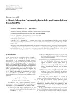
5.2. Modeling Multiprocessors Architectures. In what follows,
we present how the CPN basic models can be used to
represent and evaluate more complex system architectures.
In particular, this section presents a shared memory multiprocessor architecture, in which each microcontroller has
its own MAM latches (acting as very small cache devices).
Hence, this case study presents a study of a hierarchical
shared memory multiprocessor architecture, where each
microcontroller has a three-phase pipeline. Thus, consider

a hardware platform with two LPC2106 sharing an external
memory (see Figure 11(a)). The external memory interface
can only sustain one write access every two cycles, whereas
no such limitation exists for read accesses. Incoming requests
are placed in a queue and processed in a First In-First Out
policy. It is important to remember that each LPC2106 is also
connected to two private memories containing program code
and data.
The hardware platform described above was modeled
by replicating the model already presented for the LPC2106
and creating a new building block to represent the external
memory. Figure 11(b) depicts the proposed model for this
environment, and Figure 12 presents the external memory
model. Figure 12 also presents the CPN declarations for the
external memory. Incoming requests to the external memory
are placed in a queue in e1 (Figure 11(b)). Transitions read
mem or write mem (see Figure 12) become enabled whenever
there are incoming requests in the queue of place ext1.


EURASIP Journal on Embedded Systems

11
Table 3: Bubblesort typical scenarios results.

best-case
average-case
worst-case

Estimated

2414.6
4086.6
6162.3

Execution Time (μs)
Measured
2432,5
4247,8
6138.3

Table 4: Multiprocessor evaluation results.
Evaluation
Energy
Execution
time (s) consumption (μJ) time (μs)
one adpcm
(one microcontroller)
two adpcms
(two microcontrollers)

6

1065.77

12397.3

17

2408.5

13118.4

When read mem or write mem is fired, the correspondent
energy consumption and delay are computed.
This model was evaluated using the adpcm experiment,
where one adpcm code runs on each microcontroller. We
also assumed that 30% of the memory instructions access
the external memory. Table 4 shows the results (line 2) of
this experiment as well as the results (line 1) regarding
the execution of one adpcm in just one microcontroller
(already show in Table 1). Comparing the two results,
the energy consumption almost doubled, since besides the
energy consumption of the external memory, two processors
consume more energy than just one. On the other hand, the
execution time remained almost the same. Actually, since
the external memory introduces a bottleneck, there is a
slightly increase in this value. However, as in line 1 just one
adpcm is running, the reader should note the execution time
improvement in the parallel execution of two adpcms codes
in comparison to the sequential execution of these codes.

6. Conclusions
This work presented a method for evaluating energy consumption and performance in embedded systems. The proposed method adopts Coloured Petri Nets for modeling the
functional behavior of processors and memory architectures
at a high-level of abstraction. Further, the workload under
evaluation is mapped into the hardware model to carry
out the performance and energy consumption estimation. A
tool, named PECES, was implemented for automatizing the
method. Additionally, a measuring platform, named AMALGHMA, was constructed for characterizing the platform
and for comparing the respective results provided by the

proposed method.
This work adopted a real-world embedded platform as
case study, and the experimental results show that the proposed approach may be used to ensure a rapid and reliable
feedback to the designer. Besides, applications of the method,
such as the modeling of multiprocessor architectures, were
demonstrated. As future work, we plan to improve PECES

Error
0.74%
3.94%
0.39%

Estimated
2028.9
3453.4
5189.8

Energy Consumption (μJ)
Measured
2015.6
3634.4
5247.6

Error
0.66%
5.24%
1.11%

for helping the designer in the platform model construction
and to validate the method in other architectures.

References
[1] V. Tiwari, S. Malik, and A. Wolfe, “Power analysis of embedded
software: a first step towards software power minimization,”
IEEE Transactions on Very Large Scale Integration (VLSI)
Systems, vol. 2, no. 4, pp. 437–445, 1994.
[2] D. Brooks, V. Tiwari, and M. Martonosi, “Wattch: a framework
for architectural-level power analysis and optimizations,” in
Proceedings of the 27th Annual International Symposium on
Computer Architecture (ISCA ’07), pp. 83–94, June 2000.
[3] G. de Almeida Callou, P. Maciel, E. de Andrade, B. Nogueira,
and E. Tavares, “A coloured petri net based approach for
estimating execution time and energy consumption in embedded systems,” in Proceedings of the 21st Annual Symposium on
Integrated Circuits and System Design, pp. 134–139, 2008.
[4] E. Senn, J. Laurent, N. Julien, and E. Martin, “Algorithmic level
power and energy optimization for DSP applications: SoftExplorer,” in Proceedings of the IEEE International Symposium on
Image/Video Communications (ISIVC ’04), 2004.
[5] W. Ye, N. Vijaykrishnan, M. Kandemir, and M. J. Irwin,
“The design and use of SimplePower: a cycle-accurate energy
estimation tool,” in Proceedings of the 37th Design Automation
Conference (DAC ’00), pp. 340–345, June 2000.
[6] K. Jensen, Coloured Petri Nets: Basic Concepts, Analysis Methods, and Practical Use, Springer, New York, NY, USA, 1992.
[7] T. Murata, “Petri nets: properties, analysis and applications,”
Proceedings of the IEEE, vol. 77, no. 4, pp. 541–580, 1989.
[8] L. Wells, Performance analysis using coloured petri nets, Ph.D.
thesis, University of Aarhus, July 2002.
[9] C. Bleakley, M. Casas-Sanchez, and J. Rizo-Morente, “Software
level power consumption models and power saving techniques
for embedded DSP processors,” Journal of Low Power Electronics, vol. 2, no. 2, pp. 281–290, 2006.
[10] V. Tiwari and M. T.-C. Lee, “Power analysis of a 32-bit

embedded microcontroller,” VLSI Design, vol. 7, no. 3, pp.
225–242, 1998.
[11] M. N. Oliveira Jr., S. Neto, P. Maciel et al., “Analyzing software
performance and energy consumption of embedded systems
by probabilistic modeling: an approach based on coloured
petri nets,” in Proceedings of the 27th International Conference
on Applications and Theory of Petri Nets and Other Models
of Concurrency (ICATPN ’06), vol. 4024 of Lecture Notes in
Computer Science, pp. 261–281, 2006.
[12] J. Laurent, E. Senn, N. Julien, and E. Martin, “Highlevel energy estimation for DSP systems,” in Proceedings of
the International Workshop on Power and Timing Modeling,
Optimization and Simulation (PATMOS ’01), pp. 311–316,
Yverdon-Les-Bains, Switzerland, September 2001.
[13] A. Zimmermann, Stochastic Discrete Event Systems: Modeling,
Evaluation, Applications, Springer, New York, NY, USA, 2007.


12
[14] C. Cassandras and S. Lafortune, Introduction to Discrete Event
Systems, Springer, New York, NY, USA, 2008.
[15] G. Bolch, S. Greiner, H. de Meer, and K. Trivedi, Queueing
Networks and Markov Chains, Wiley-Interscience, New York,
NY, USA, 2005.
[16] W. Stewart, Probability, Markov Chains, Queues, and Simulation: The Mathematical Basis of Performance Modeling,
Princeton University, Princeton, NJ, USA, 2009.
[17] C. Hirel, R. Sahner, X. Zang, and K. Trivedi, “Reliability
and performability modeling using sharpe,” in Proceedings of
the 11th International Conference on Computer Performance
Evaluation. Modelling Techniques and Tools, vol. 1786 of
Lecture Notes in Computer Science, pp. 345–349, Schaumburg,

Ill, USA, March 2000.
[18] A. Vinter Ratzer, L. Wells, H. Lassen et al., “CPN tools for
editing, simulating, and analysing coloured petri nets,” in
Proceedings of the 24th International Conference on Applications
and Theory of Petri Nets, vol. 2679 of Lecture Notes in Computer
Science, pp. 450–462, Springer, Eindhoven, The Netherlands,
2003.
[19] ARM Limited, “ARM7TDMI-S Technical Reference Manual
(Rev. 4),” 2001.
[20] Philips Electronics, “NXP LPC2104, LPC2105, LPC2106 Data
Sheet,” 2004.
[21] D. Lilja, Measuring Computer Performance: A Practitioner’s
Guide, Cambridge University Press, Cambridge, UK, 2005.
[22] Keil, “Gcc compiler,” />.htm.
[23] M. Westergaard and L. Kristensen, “The access/CPN framework: a tool for interacting with the CPN tools simulator,” in
Proceedings of the 30th International Conference on Applications
and Theory of Petri Nets, vol. 5606 of Lecture Notes in Computer
Science, pp. 313–322, Springer, 2009.

EURASIP Journal on Embedded Systems