Báo cáo hóa học: " Research Article Adaptive Resource Allocation with Strict Delay Constraints in OFDMA System" ppt

Hindawi Publishing Corporation
EURASIP Journal on Wireless Communications and Networking
Volume 2010, Article ID 121080, 14 pages
doi:10.1155/2010/121080

Research Article
Adaptive Resource Allocation with Strict Delay Constraints in
OFDMA System
Naveed Ul Hassan and Mohamad Assaad
Department of Telecommunications, Ecole Sup´rieure d’Electricit´ (Sup´lec), Plateau de Moulon, 3 rue Joliot Curie,
e
e
e
91192 Gif-sur-Yvette Cedex, France
Correspondence should be addressed to Naveed Ul Hassan,
Received 18 September 2009; Revised 20 April 2010; Accepted 5 August 2010
Academic Editor: A. Lee Swindlehurst
Copyright © 2010 N. Ul Hassan and M. Assaad. This is an open access article distributed under the Creative Commons Attribution
License, which permits unrestricted use, distribution, and reproduction in any medium, provided the original work is properly
cited.
We consider the adaptive resource allocation problem in downlink Orthogonal Frequency Division Multiple Access (OFDMA)
system with strict packet delay constraints in the range of 1 < D < ∞. In this range of delay constraints, resource optimization
has to be simultaneously performed over multiple time slots. Thus optimal allocation decisions require future Channel State
Information (CSI) and packet arrival rate information. The causal nature of CSI combined with the increase in the number
of optimization variables makes it a very challenging problem. We propose a two-step solution by separating scheduling from
subcarrier and power allocation. Our proposed causal scheduler ensures delay guarantees by deriving a minimum data rate out of
the user queues while minimizing transmit power in every time slot. The output rates are fed to the resource allocation block and
the problem is formulated as a convex optimization problem. The subcarrier and power allocation decisions are made in order
to satisfy the demanded rates within the peak power constraint. We address the feasibility of the physical layer resource allocation
problem and develop efficient algorithms. When the problem is infeasible we devise a strategy which incurs minimum deviation
from the proposed rates for maximum number of users. We show by simulations that our proposed scheme can efficiently utilize

time variations as well as multiuser diversity in the system.

1. Introduction
Harsh wireless channel conditions, scarce bandwidth,
and limited power resources require intelligent allocation
schemes which can efficiently exploit channel variations.
OFDMA is a multicarrier modulation and multiplexing
technique which divides the wideband frequency selective
wireless channel into a set of orthogonal narrowband channels and provides immunity from Intersymbol Interference
(ISI) [1]. In a multiuser system, different subcarriers can be
allocated to different users without interference. Due to the
multi-carrier nature of OFDMA systems, enormous opportunities exist for dynamic subcarrier and power allocation
strategies [2–4].
Most of the existing work on adaptive resource allocation
schemes in OFDMA systems has focused on traffic types with
delay constraints of either D = ∞ or D = 1. D = ∞ represents
the delay tolerant traffic while D = 1 represents the delay

intolerant traffic. In both these cases (D = 1 and D = ∞),
optimal subcarrier and power allocation decisions require
instantaneous CSI only [5–7]. It is obvious that D = ∞ and
D = 1 are in fact two extreme cases and do not represent
practical service types. For all the practical service types,
packet delay constraints are always in the range of 1 < D < ∞.
In this range of delay constraints, it is possible to exploit the
short-term channel time variations. However, the resource
allocation decisions depend on current as well as the future
values of packet arrival and channel state information. The
future traffic and channel state information is generally not
available due to causality constraints. Moreover, this problem

has a larger state space, an increased number of optimization
variables, and the stochasticity in the arrival process and
channel variations make it much harder to exploit time
diversity and thus make this problem very challenging.
In this paper, we propose a two-step solution to sumrate maximization problem with strict delay constraints in


2

EURASIP Journal on Wireless Communications and Networking

the range 1 < D < ∞. A Minimum Rate Scheduler (MRS) is
developed which conceals the delay constraints in the form of
data rate constraints while in the second step subcarrier and
power allocation decisions are made based on the data rates
proposed by the scheduler. We compare the performance
of our physical layer resource allocation algorithm with the
solution proposed in [8]. By using a greedy algorithm, the
authors estimate the required resources based on average
channel gains of the users in the first step while in the second
step exclusive subcarrier assignments are made based on the
Hungarian algorithm [9, 10].
1.1. Previous Work. When D = 1 scheduling is not required.
Several schedulers have been developed in [11–15] for the
case when D = ∞. Some of these schedulers [11, 12] base
their scheduling decisions entirely on the current CSI and
are known as the Channel-Aware Only (CAO) schedulers.
CAO schedulers provide long-term fairness without ensuring
strict delay guarantees for any packet in the system. The
second class of schedulers employ both the channel and the

queue state informations to incorporate fairness among users
[13–15]. Modified Largest Weighted Delay First (M-LWDF)
rule [14] and the Exponential (Exp) Rule [15] schedulers
are Channel-Aware Queue-Aware (CAQA) schedulers. These
schedulers perform significantly better than CAO schedulers
but they are also unable to respect strict packet delay
constraints. Scheduling is separated from subcarrier and
power allocation in [16–18]. However, the objective of the
authors in these papers is the average delay minimization
rather than strict delay constraint achievement. In [19],
the authors consider packet scheduling with strict delay
constraints for AWGN channels and derive robust energy
efficient schedulers. The authors in [20, 21] exploit energy
delay tradeoff and propose strategies to minimize queuing delay for single-user single-carrier systems. Similarly
dynamic programming was adopted in [22] for scheduling
packets over a time-slotted single-user wireless link. Perhaps
the work in [23] for TDMA systems is closest to our approach
in terms of problem formulation. In this paper, the authors
develop energy efficient scheduler with individual packet
delay constraints by developing bounds on transmission rate
and then write the optimization problem. However, their
work is again limited to TDMA systems and there is no power
control in their developed schemes.
We want to stress that the specific optimization problem
of sum rate maximization subject to strict individual user
delay constraints is largely ignored due to the larger state
space size of the problem. In general, good schedulers to
achieve strict delay constraints when 1 < D < ∞ for
multiuser OFDMA systems are largely missing and this paper
is an effort to fill this gap.

1.2. Proposed Approach and Main Contributions. In this
subsection we highlight our proposed solution and the main
contributions of this paper.
(i) The problem of achieving strict target delay constraints is stretched in the past and in the future and
we can capture this dependence by developing certain

bounds on data rate transmission in each time slot.
We develop two bounds (upper and lower bound
constraints) which help us to write the resource
allocation problem.
(ii) We write the adaptive resource allocation problem
with strict delay constraints in OFDMA systems as an
optimization problem. The objective of the problem
is to maximize the sum-rate in D = max{D1 , . . . , DK }
time slots. The problem formulation is flexible to
accommodate different services for different users
in the system. We develop a suboptimal two-step
solution to solve this problem. We develop MRS
which propose an instantaneous data rate for each
user in each time slot and then we maximize the
instantaneous sum-rate in the next step.
(iii) The objective of MRS is to propose a minimum
data rate for each user which is just sufficient to
attain strict delay constraints of the packets. If we can
attain these data rates at the physical layer without
violating the peak power constraint strict delays are
guaranteed. In fact there are three possibilities as
follows.
(a) The proposed rates are achieved at the physical
layer and all the available power gets consumed

in achieving these rates.
(b) The proposed rates are achieved and there is
some power still left at the BS. In this case, the
remaining power is allocated to the best users
in the systems. Thus we maximize the sumrate without fearing the delay violations of the
packets.
(c) The proposed rates cannot be achieved with
the given amount of power. In this case, the
data rates proposed by MRS are not feasible.
We develop an algorithm where we decrease
the data rates of some of the users. However,
for such users the backlog is high for next
time slots. Hence, MRS will adapt its decisions
according to the backlog information and tries
to compensates this loss in future time slots.
MRS solves a sum-power minimization problem. The
optimization problem for MRS is formulated over
D time slots. In order to reduce the complexity
T
we take average power in future time slots. This is
sub-optimal but the effects due to sub-optimality are
corrected in the next time slot by utilizing the backlog
information. Thus by using QSI, MRS tracks the
actual channel conditions and corrects its decisions.
(iv) Once we have the target data rates proposed by the
MRS, the remaining problem is an instantaneous
optimization problem. However, since we have limited amount of transmission power available at the
BS hence there is an issue of feasibility. We develop
a method to detect the nonfeasibility in the problem.
Then we propose algorithms for the feasible and nonfeasible cases. MRS decisions are thus corrected by

the physical layer algorithms.


EURASIP Journal on Wireless Communications and Networking
(v) It should be noted that we do not use Dynamic
Programming (DP) or some other probabilistic optimization techniques in this paper. DP depends on
the probability distribution function (pdf) of the
arrivals (traffic and channels) and future allocations.
The state space equation is easier to write for simple
pdf functions like Bernouilli, Gaussian, or Brownian
process. Since the future channels and traffic can have
more elaborated pdf functions and it is hard to find
the pdf of the allocation in the future time slots, thus
it is difficult to write the problem using a state space
equation. Moreover the use of DP is restricted by
the number of variables in the optimization problem
since they increase the number of state space variables. Since in our problem we have power allocation,
plus exclusive subcarrier assignment constraint over
D time slots thus the state space of our problem is
very huge and dynamic programming techniques are
not feasible.
The rest of the paper is organized as follows. In Section 2,
system model is described and the problem is formulated. Section 3 details the causal scheduler which derives
minimum data rates for the users. Physical layer resource
allocation algorithm and feasibility issues are discussed in
Section 4. Complexity analysis of the scheduler and the
resource allocation algorithms is carried out in Section 5
while simulation results are presented in Section 6. Finally,
the paper is concluded in Section 7.

2. System Model and Problem Formulation
We consider a downlink OFDMA system with K users and
F subcarriers. We assume that the total transmit power
from the BS is constrained to Pmax . Time is divided into
slots and during each time slot a data frame consisting of
M OFDM symbols is transmitted. User channels remain
constant for the duration of a time slot but may change from
one time slot to another. We assume that perfect Channel
State Information (CSI) is available at the BS. The channel
t
gain to noise ratio gk, f of user k on subcarrier f during
t
time slot t is given by gk, f = |ht f |2 /N0 B, where |ht f |
k,
k,
denotes the channel coefficient of user k on subcarrier f
after Fast Fourier Transform (FFT), N0 is the power spectral
density (PSD) of white noise, and B denotes the bandwidth
of single subcarrier. Each user maintains a separate queue at
the BS which receives data from the higher layer. We assume
that all the packets of user k have same delay constraint
which is in terms of number of time slots and denoted by
Dk (different users have different packet delay constraints).
Therefore, packets of user k arriving at time t must be out
of the queue before the start of time slot t + Dk , otherwise
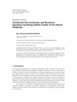
they are dropped. The system model is detailed in Figure 1.
Each user has a separate MRS scheduler which derives a
minimum rate based on the available channel and Queue
State Information at the start of each time slot. Resource
allocation algorithm is employed which allocates power and

subcarriers according to the minimum rates and peak power
constraint. This assignment information is sent to the users

3

via separate control channels which allow the users to recover
their data.
t
Let Rt and Xk be the output rate and the input arrival
k
t
rate of user k at time t, the queue backlog Bk then evolves
according to the following equation:
t+1
t
t+1
Bk = Bk + Xk − Rt
k

+

∀k.

,

(1)

Without any loss of generality we assume that we start at time
t = 1 and that the initial backlog is zero. The backlog at the
start of time slot t for user k is

t
t
1
Bk = Xk − R1 + · · · + Xk−1 − Rt−1
k
k

(2)

t −1

=
i=1

i
Xk − Rik ,

∀k.

We assume that the packets are dropped if they cannot be
delivered before their delay deadline which means that at
t+1
time t, Bk −Dk = 0. In order to ensure strict delay constraint
Dk for all the packets, we must impose certain conditions on
the output data rate of each user k at each time slot t. Below
we derive these necessary conditions,
2.1. Lower Bound Constraint. Since all the packets of user k
have same delay constraint Dk , we have
t
1

Xk + · · · + Xk ≤ R1 + · · · + Rt + · · · + Rt+Dk −1 ,
k
k
k

∀k.

(3)
Therefore, at any time t the output rate Rt must satisfy the
k
following constraint:

i=1

t+Dk −1

t −1

t

Rt ≥
k

i
Xk −

i=1

Rik −

i=t+1

Rik ,

∀k.

(4)

Finally, we can write that
t+Dk −1
t
t
Rt ≥ Bk + Xk −
k

i=t+1

Rik ,

∀k.

(5)

This constraint ensures that a packet arriving at time t
will be out of the buffer before t + Dk − 1. Equation (5)
gives a lower bound on the output data rate. We have to
proceed sequentially in time to derive the optimal output
rates. Moreover, the dependence of Rt on future allocation
k
decisions is explicit from this constraint.

2.2. Upper Bound Constraint. This constraint arises from the
fact that a packet cannot be transmitted before its arrival.
Therefore, packets arriving at time t should be transmitted
either during this time slot or future time slots, that is,
t
1
R1 + · · · + Rt ≤ Xk + · · · + Xk ,
k
k

∀k.

(6)

The condition on output rate becomes
t
t
Rt ≤ Bk + Xk ,
k

∀k.

Equation (7) gives an upper bound on Rt .
k

(7)


4

EURASIP Journal on Wireless Communications and Networking

2.3. Optimization Problem. Since this is an OFDMA problem
t
we assume that Ik are the subcarriers allocated to user k
during time slot t. By using the Shannon capacity formula,
the data rate achieved by user k on its allocated subcarrier set
t
Ik during time slot t is given as ( data rates are expressed in
nats for analytical convenience)
t
t
Rt pk, f , gk, f =
k

t
t
log 1 + pk, f gk, f nats/s/Hz,
t
f ∈Ik

(8)

t
where pk, f is the power allocated to user k on subcarrier f
during time slot t. We now write an optimization problem in
order to determine the optimal output rates and to allocate
the subcarriers and powers to different users. Let D =
max{D1 , . . . , DK }. In order to achieve the target packet delay
constraints, we have the following optimization problem:

t+D−1 K

max
i=t k=1

i
i
Rik pk, f , gk, f

(9)

t,k
propose a minimum data rate Rmin for each user according
to constraints (10) and (11). The instantaneous subcarrier
and power allocation decisions are then made by solving
a constrained instantaneous sum-rate maximization problem.( There are some instantaneous constraints in the above
optimization problem. These constraints remain the same
and do not affect the two-step approach. The peak power
constraint has to be attained in each time slot as well as the
OFDMA constraints. We replace the upper and lower bound
constraints by the minimum data rate constraints. Now if
the data rates proposed by the scheduler are optimal the two
step approach is completely justified. Due to approximations
and the complexity of our problem the scheduler is not
optimal hence there is some performance loss. However,
some of this performance loss is compensated by the physical
layer algorithm.) In this problem, the proposed data rate
vector by the scheduler is an additional constraint along with
constraints (12), (13) and (14). The instantaneous sum-rate
problem is as follows:

K

subject to

t
t
Rt f pk, f , gk, f
k,

max
i+Dk −1

i
i
i
i
Rik pk, f , gk, f ≥ Bk + Xk −

t
t
Rt pk, f , gk, f
k

∀k, i,

t=i+1

subject to

(10)

Rik

i
i
pk, f , gk, f

≤

i
Bk

i
+ Xk

∀k, i,

(11)

(15)

t
k=1 f ∈Ik

t,k
t
t
Rt f pk, f , gk, f ≥ Rmin
k,

∀t, k,

t
f ∈Ik

(16)

K
t
pk, f ≤ Pmax ,

K
i
pk ≤ Pmax ,

∀i,

(12)

t
t
Im ∩ In = Φ,

k=1
i
Im

i
∩ In

= Φ,

∀m = n,
/

∀i,

(13)

i
Ik

⊆ {1, . . . , F },

∀m = n,
/

∀i.

(14)

k=1

The objective of the problem in (9) is the throughput
maximization or system capacity which is the main goal of
the network operators. Constraints (10) and (11) are the
instantaneous constraints on the data rate of each user in
order to ensure strict delay constraints. These constraints
correspond to the lower bound (5) and the upper bound
(7) on the output data rates, respectively. Constraint (12)
demands that the total transmit power should always be less

than the peak power constraint in each time slot. Constraints
(13) and (14) are the OFDMA constraints which demand
that at any time t each subcarrier should be allocated to no
more than one user and that the sum of all the subcarriers
should be equal to the total number of subcarriers in the
system.
To get an optimal solution we need to find the optimal
output rates Rt , for all t, k. This problem is nonconvex
k
and is not easy to solve because the optimal value of Rt
k
in (10) is bounded by unknown variables which depend
on future allocation decisions as well as future channel
gains and future input arrival rates. We develop a twostep solution to solve this problem. We develop MRS which

(17)

∀t,

(18)

K
t
Ik ⊆ {1, . . . , F },

K

∀t,

t

k=1 f ∈Ik

∀t.

(19)

k=1

Equation (16) is the instantaneous data rate constraint. If
the data rates achieved by the resource allocation algorithm
t,k
are equal to or greater than the proposed data rates Rmin ,
for all k, then delay constraints are satisfied. However, if in
any time slot these data rates cannot be achieved due to bad
channel conditions and power limitations then this loss is
compensated for by the MRS in the next time slot. Hence,
time diversity in the wireless channel is utilized since D > 1.
Moreover, since we are maximizing the instantaneous sumrate in (15) therefore the long term objective in (9) is also
maximized. In the next section, we develop the Minimum
t,k
Rate Scheduler to derive Rmin .

3. Minimum Rate Scheduler
We are interested in developing a scheduler which can propose minimum data rates such that strict delay constraints
are guaranteed. From Figure 1, we can see that scheduler
works in advance of subcarrier and power allocation block.
Since actual transmitted power is not decided by the
scheduler therefore we will base our scheduling decisions on
transmit power minimization. Power minimization can be

EURASIP Journal on Wireless Communications and Networking

5

Base station

User k

R1
R2
CSI

CSI
MRS

QSI

CSI

OFDM
transceiver

OFDM
transceiver

CSI

Data
user k

Rk

MRS

QSI

Data

MRS
QSI

Subcarrier
and power
allocation

User k

User 1 User 2

CSI

Subcarrier
and power
allocation
algorithm

Subcarrier
information
Subcarrier

information
for user k

Subcarrier
selector

QSI: queue state information
CSI: channel state information
MRS: minimum rate scheduler

Figure 1: System model.

seen as a useful way of enhancing sum-rate during resource
allocation process. An optimal scheduler is able to to fully
exploit the leverage provided by the delay constraints and at
any time instant t it schedules a minimum rate out of the
buffer which is able to satisfy all the delay constraints. If this
is not the case then scheduling more packets than required
will result in huge increase in power. So the name MRS
comes from the fact that the scheduled rates are the lowest
possible data rates which ensure strict delay guarantees while
consuming the least amount of power. If these minimum
rates can be achieved then the remaining power can be
strictly utilized in enhancing the system capacity without
worrying about delay violations. Thus the objective of MRS
is the minimization of total transmit power subject to
achieving strict delay constraints of the packets.
Since each user has a separate scheduler so in the
subsequent analysis we will drop the user index for simplicity.
During each time slot t we solve the optimization problem

for MRS in a very large interval [t, t + T]. We call T the
1, T
D, for all k. The
optimization interval where T
reason behind solving the optimization problem for T time
t,k
slots is to make explicit the dependence of Rmin on future
arrival rates. Since the delay constraints of packets arriving at
time slot t +T is D, hence the summation is over t +T +D − 1.
In fact this formulation for MRS problem has been inspired
from the work in [23]. The optimization problem for MRS is
as follows:
t+T+D−1

min pt +

pi
i=t+1

(20)

subject to
t+T+D−1

Rt pt , g t +

t+T

Ri pi , g i = Bt + X t +
i=t+1

X i,

(21)

i=t+1
t+D−1

Rt pt , g t ≥ Bt + X t −

Rd pd , g d ,

(22)

d =t+1

Rt pt , g t ≤ Bt + X t .

(23)

Due to causal nature of the scheduler and the fact that
optimization interval T is assumed to be sufficiently large,
at any time t the problem can be written as
min pt + (T + D − 1)p

(24)

subject to
Rt pt , g t + (T + D − 1)E R p, g

= B t + X t + (T)X0 ,

(25)
Rt pt , g t ≥ Bt + X t − (D − 1)E R p, g ,

(26)

Rt pt , g t ≤ Bt + X t .

(27)

The objective in (24) is the average power minimization in
the optimization interval. Constraint (25) ensures that all the
packets arriving in the optimization interval are transmitted
before their delay deadlines. Constraints (26) and (27) are
again the lower and upper bounds on the data rates. In this
optimization problem, p and X0 denote the mean power
and the mean input arrival rate while E[R(p, g)] is the


6

EURASIP Journal on Wireless Communications and Networking

mean output rate estimated at time t. The above problem
is not convex due to the presence of bounding constraints.
We propose a heuristic solution where in order to get a
good starting point we solve the problem by ignoring the
bounding constraints (26) and (27). This problem results in
output rate which may or may not be satisfying the bounding

constraints. However, once this data rate is obtained, it
is used in subsections A to C to get minimum output
rate satisfying constraints (26) and (27). We observe that
E[R(p, g)] is a function of two random variables that is, g
and p. By Jenson’s inequality we have
Eg,p R p, g

≥ Eg R p, g

= Eg log 1 + pg

,

(28)

where Eg [R(p, g)] is the lower bound on the expected values
of future output rates which will ensure that the minimum
required rate over D time slots will be achieved. With this
approximation, the relaxed optimization problem without
constraints (26) and (27) can be written as
min pt + (T + D − 1)p

(29)

subject to
log 1 + pt g t + (T + D − 1)Eg log 1 + pg

(30)

= B t + X t + (T)X0 .

This optimization problem can be solved using the Lagrange
optimization techniques since the objective and the single
constraint function are convex and KKT conditions are
sufficient to arrive at the solution [24]. Let β be the Lagrange
multiplier associated with the constraint, the Lagrangian is,
L pt , p = pt + (T + D − 1)p
− β log 1 + pt g t

(31)

+ (T + D − 1)Eg log 1 + pg
−B t − X t − (T)X0 .

βEg

=

0 and

gt
1 + pt g t

= 1,

(32)

g
1 + pg

= 1.

(33)

Let, f1 (p) = Eg [g/1 + pg] and f2 (p) = Eg [log(1 + pg)]. From
(33), we have
β=

1
.
f1 p

(34)

Similarly, from (32), we have log(1 + pt g t ) = log(βg t ) so we
can rewrite (30) as
gt
log
f1 p

t

(1) Numerically solve (35) to get the value of p.
(2) For this value of p, find β using (34).
(3) The output rate at time t is Rt = log(βg t ).
(4) The anticipated scheduled rates for future time slots at time t
are, log(βg0 ), where g0 is the mean channel gain value.

Based on the previus equations we develop an algorithm
which we will refer to as the MRS algorithm to find the

value of Rt provided the probability density function (pdf)
of the underlying physical channel is known. This algorithm
is given in Table 1. It should be noted that the scheduled
rates are not the actual future output rates because their
exact values cannot be determined until that future time is
reached. The value of interest is the current output rate Rt
which may not be satisfying the two constraints given in (26)
and (27).
Remark. f1 (p) and f2 (p) depend on the nature of the
underlying physical channel and can be determined if
the probability density function (pdf) of random channel
variable g is known. Thus, the solution developed in this
section is quite general and can be used for any type of
channel as long as channel pdf is known and f1 (p) and f2 (p)
are computable.
Example. As an example, we determine the values of f1 (p)
and f2 (p) by assuming the underlying channel to be Rayleigh
fading. In this case, random variable g is exponentially
distributed with mean g0 and probability density function
given by 1/g0 e−g/g0 . With f1 (p) and f2 (p) defined on the
interval [0, ∞), we have
f1 p =
f2 p =

From KKT conditions ∂L{ pt , p}/∂pt
∂L{ pt , p}/∂p = 0, we get
β

Table 1: MRS algorithm.

t

+ (T + D − 1) f2 p = B + X + (T)X0 .
(35)

ge−g/g0 dg
g0 p − e1/g0 p Ei 1/g0 p
=
,
g0 1 + pg
g0 p 2

1
log 1 + pg e−g/g0 dg = e1/g0 p Ei 1/g0 p ,
g0
(36)

where Ei is the exponential integral function, defined as
∞
Ei(p) = p e− p d p/ p, p > 0.
Since the output rate has to satisfy both the upper and the
lower bound constraints hence there are three possibilities
for the value of Rt attained by the above algorithm. Let, x =
Rt , y = Bt + X t , and z = (D − 1)E[R(p, g)] in the constraint
equations (26) and (27), then these three cases are as follows.
3.1. Case I: x ≤ y and x ≥ y − z. In this case, both the
t,k
constraints are satisfied so Rmin = Rt is a valid minimum
rate.
3.2. Case II: x > y. Constraint (27) is violated because

the proposed output rate is higher than total number of
packets available for transmission. The output rate is high
because the channel is good. Therefore, valid strategy is to


EURASIP Journal on Wireless Communications and Networking
transmit all the available packets in this time slot. We reduce
t,k
the output rate and make it equal to y, that is, Rmin =
t + X t . It is obvious that by decreasing Rt , constraint (26)
B
is not violated because all the packets are scheduled for
instantaneous transmission.
3.3. Case III: x ≤ y and x < y − z. In this case, constraint
(26) is violated so the delay deadlines of the packets are not
achieved. The output rate is less than what is required to
ensure the delay constraints. Therefore, we have to increase
x or z so that x + z = y. The problem can be viewed as
rescheduling y packets over D time slots which is equivalent
to the unconstrained problem in the optimization interval
[t, t + D − 1]:
min pt + (D − 1)p

7

total transmit power subject to minimum rate constraints.
On the other hand, rate-adaptive objective has no minimum
rate constraints as it maximizes the sum-rate subject to
peak power constraint. Moreover, this optimization problem
is a combinatorial problem due to the fact that users

cannot share the same subcarrier. The combinatorial nature
of the problem can be avoided by allowing the users to
time-share each subcarrier over an OFDM symbol [2]. We
t
introduce a time sharing factor γk, f ∈ [0, 1] for kth user on
subcarrier f . During an OFDM symbol user k is allowed to
t
transmit on subcarrier f for γk, f percentage of time. This is
possible from resource allocation point of view because we
have assumed that channel remains constant in each time
slot. This assumption on subcarrier sharing introduces the
following constraint:

(37)
K

subject to

t
γk, f ≤ 1,
t

R + (D − 1)E R p, g

= y.

(38)

This problem can be solved on similar lines to the relaxed
problem discussed before and the same algorithm can be

used. The resulting value of Rt is now a valid output
rate which satisfies both the constraints. It is important to
mention here that since we are proceeding sequentially in
time so we are achieving delay constraint in every time slot.
Since x + z = y, therefore, constraint (27) cannot be violated.
It should be noted that both constraints cannot be
violated at the same time because they represent the upper
and the lower bounds. After obtaining the minimum rates
we pass them to the physical layer resource allocation block.

4. Physical Layer Resource Allocation
t,k
Let Rmin be the data rate passed by each MRS to physical layer.
The optimization problem during any time slot is,

⎛

Rt f
k,

t
t
t
pk, f , γk, f , gk, f

=

t
γk, f

log⎝1 +

⎛

K

t
γk, f log⎝1 +

max

(39)

t
γk, f

t
t
pk, f gk, f

f =1k=1

t
k=1 f ∈Ik

subject to

t
t
pk, f gk, f

⎞
⎠.

(45)

Equation (45) represents a concave function which can be
verified from its Hessian which is negative semidefinite when
t
t
γk, f ≥ 0 and pk, f ≥ 0. Finally, we can write the optimization
problem as
F

t
t
Rt f pk, f , gk, f
k,

(44)

As a result of time sharing, data rate achieved by user k on
t
t
t
t
t
subcarrier f becomes Rt f (pk, f , gk, f ) = γk, f log(1 + pk, f gk, f ).
k,
This function is neither convex nor concave. Therefore we

t
t
t
define pk, f = γk, f pk, f as the average power allocated to user
k on subcarrier f . With this change of variable, we have

K

max

∀f.

k=1

t
γk, f

⎞
⎠

(46)

subject to
Rt f
k,

t
t
pk, f , gk, f

≥

t,k
Rmin

∀t, k,

t
f ∈Ik

(40)
F

K
t
pk, f

≤ Pmax ,

∀t,

(41)

t
k=1 f ∈Ik

t
t
Im ∩ In = Φ,

⎛
t
γk, f log⎝1 +

t
t
pk, f gk, f )
t
γk, f

f =1

⎞
⎠ ≥ Rt,k ,
min

∀k,

(47)

K

∀m = n,
/

∀t,

(42)

K

t
γk, f ≤ 1,

∀t.

This problem can be viewed as a combination of marginadaptive and rate-adaptive optimization problems. It is
important to mention here that margin adaptive objective
does not include power constraint as it tries to minimize

(49)

K

(43)

k=1

(48)

t
pk, f ≤ Pmax .

F
t
Ik ⊆ {1, . . . , F },

∀f,

k=1

f =1k=1

This is a convex optimization problem with linear and convex differentiable constraints. We can solve it by using convex
t
optimization theory [24, 25]. Let (δk )k=1,...,K , (μtf ) f =1,...,F and


8

EURASIP Journal on Wireless Communications and Networking

αt be the Lagrange multipliers associated with constraints
(47), (48), and (49), respectively. The Lagrangian is
K

L

t
t
pk, f , γk, f

t
1 + δk

=
k=1

⎧
⎨

⎩

⎛

F
t
γk, f

t t,k
δk Rmin

−

t⎝

t
pk, f

P (R) = {Pt : (Ck = Rk , ∀k)}.

− Pmax ⎠

⎛

f =1

K

⎞
t

γk, f ⎠ − 1).

k=1

(50)
Since the objective and constraint functions are convex
the duality gap is zero and we can use Lagrange dual
decomposition theory to solve this problem. The dual
problem is to maximize

K

G

= maximize L

t
t
pk, f , γk, f

.

⎛

t
t
t
Sk, f δk , αt , μtf = 1 + δk ⎩γk, f log⎝1 +
t
t

− αt pk, f − μtf γk, f

t
t
pk, f gk, f
t
γk, f

⎛
t
γk, f

(52)

∀k, f .

⎛

t
1 + δk

⎞+
t
⎝ 1 + δk − 1 ⎠ ,
=
t
t

α

gk, f

f =1

α

= μf ,

(53)
αt

t
t
1 + δk gk, f

⎞+ ⎞
⎠ ⎟
⎠

∀f.

(54)
From (53) and (54), it is extremely difficult to develop an
algorithm for subcarrier and power allocation. Moreover,
there is also a question of feasibility because given a fixed total
power, it might not be possible to support all the minimum
rates during current time slot.
4.1. Feasibility of Physical Layer Optimization Problem. Since
our problem is convex, a necessary and sufficient condition
for feasibility is the nonemptiness of the feasible set. Let

C = {C1 , . . . , Ck } be the achieved data rate vector and R =
{R1 , . . . , RK } be the rate constraint vector. Let Pt be the total
power required in achieving C. The feasible set can be defined
as
R = {C : (Ck ≥ Rk , ∀k) ∩ Pt ≤ Pmax },

t
γk, f

⎞
⎠ ≥ Rt,k ,
min

∀k,

(58)

K
t
γk, f ≤ 1,

∀f.

(59)

From our previous analysis it is evident that this is also a
t
convex optimization problem, therefore, with (δk )k=1,...,K and
t
(μ f ) f =1,...,F as the Lagrange multipliers associated with the

constraints (58) and (59), respectively. Then by solving the
Lagrange-KKT optimality conditions, we get
⎛
t
pk, f

(55)

t
δk ⎝

⎛

log

t t
δk gk, f

⎞+

1
t
= ⎝δk − t ⎠ ,
gk, f

⎛

∀k, f ,

⎛⎛ ⎛

⎞⎞+ ⎛
t
t
⎜⎝ ⎝ 1 + δk gk, f ⎠⎠
− ⎝1 −
⎝ log
t

log⎝1 +

t
t
pk, f gk, f

k=1

t
Since subproblems Sk, f (δk , αt , μtf ) are also convex,
KKT conditions are sufficient to find a solution. From
t
t
t
t
∂Sk, f (δk , αt , μtf )/∂ pk, f = 0 and ∂Sk, f (δk , αt , μtf )/∂γk, f = 0,
we arrive at
t
pk, f

(57)

subject to

(51)

⎞⎫
⎬
⎠
⎭

t
pk, f
k=1 f =1

t
We can readily decompose G(δk , αt , μtf ) on subcarriers and
users to get KF subproblems

⎧
⎨

F

min

F
t
δk , αt , μtf

(56)

Let Pmg be the optimal point of the set (56). Our problem is
feasible if Pmg ∩ R2 is nonempty which is possible if Pmg lies
inside or on the boundary of R2 . Therefore, the feasibility
issue is reduced to finding Pmg which can be obtained by
solving the following margin adaptive problem:

k=1 f =1

μtf ⎝

−

t
γk, f

⎞⎫
⎬
⎠
⎭

⎞

F

K

−α

k=1
F

t
t
pk, f gk, f

f =1

⎛

K

log⎝1 +

where R is the intersection of two sets. Let the set defined
by rate constraint vector be denoted by R1 and peak
power constraint by R2 . Each rate constraint vector has an
associated power region. Let P be the power region when
Ck = Rk , for all k, that is,

+

(60)

⎞+ ⎞

1
− ⎝1 − t t ⎠ ⎠ = μtf .
δk gk, f

(61)

Using (60) and (61), we can develop a margin adaptive
algorithm. This algorithm is very similar to the one given in
[2]. The algorithm is presented in Table 2. A set of subcarriers
I k gets allocated to each user k and power is allocated on
these subcarriers according to waterfilling principle. Step 1
of this algorithm can be used to get margin adaptive solution
for single user OFDM system. For a small enough step size
the convergence of above algorithm is surely attained [24].
There is a possibility that more than one user converge to
the same value of μtf . In this case, the optimal solution is
attained by time sharing of a subcarrier between the tied
users on each such subcarrier. These ties can be broken by
randomly picking a single user for exclusive transmission
on such subcarrier. Although this heuristic to break the ties
will lead to small deviations in QoS requirements however
it is adopted here to reduce the complexity of our proposed
solution. Moreover, the probability of this event vanishes
exponentially under some reasonable conditions as K and F
increases. Further details can be found in [26, 27].
Comparing (60) and (61) with (53) and (54) we can
see that the original problem with power constraint turns


EURASIP Journal on Wireless Communications and Networking

9

Table 2: Margin adaptive algorithm.
t

t
(1) Initialization: = mink, f 1/gk, f , ∀k, φk, f = 0, ∀k, f , γk, f = 0, ∀k, f , Γk = 0, ∀k.
(2) Repeat till all the rate constraints are achieved.
(3a) Repeat till kth user rate constraint is achieved.
t
t
(3b) Increase waterlevel of user k, δk = δk + Δm .
+
+
t
t t
t t
(3c) On all the subcarriers compute φk, f = δk ((log(δk gk, f )) − (1 − 1/δk gk, f ) ).
t
t
(3d) Allocate subcarrier to this user if φk, f is maximum and set γk, f = 1 other wise γk, f = 0.
+
F
t
t t
(4) Compute the achieved data rates according to, Γk = f =1 γk, f (log(δk gk, f )) ∀k.
t
δk

t,k, f

adaptive algorithm. We suppose that pr is the additional
power allocated to user k on subcarrier f . We can write the
following optimization problem to allocate additional power:

pr (k, f )
1/η
δ1

t,k, f

log 1 + pm

max
t
k∈Ω f ∈Ik

δ2

pm (k, f )

t,k, f

+ pr

t
gk, f

(62)

subject to

1/g(k, f )

k = 1 k =1 k = 1 k = 1 k = 1 k = 2 k = 2 k = 2

Subcarriers f = 1, . . . , 8

Figure 2: Illustration of multiuser waterfilling for 2 user 8
subcarrier system for feasible case.

t,k, f

pm

4.2. Feasible Case: Pmg ≤ Pmax . When the problem is
feasible, minimum rates can be achieved under the peak
power constraint. If Pmg < Pmax , there is more power
than required to satisfy the minimum rates. We develop a
scheme to allocate this additional power to the users. We
use margin adaptive algorithm (αt = 1) to find subcarrier
allocation. Then on the allocated subcarriers remaining
power is utilized. Let Ω be the set of users with non-empty
t,k
t+1
queues after the transmission of Rmin , that is, Bk > 0,
t,k, f
for all k ∈ Ω . Let pm be the margin adaptive power
t
allocation and Ik be the set of subcarriers assigned by margin

t,k, f

pm

+

t
k∈Ω f ∈Ik

= Pmax .

t
k ∈ Ω f ∈Ik
/

(63)

This problem is also convex, so with ηt as Lagrange
multiplier associated with the constraint (63) and solving
KKT conditions, we arrive at
⎛
t,k, f
pr

into margin adaptive problem when αt = 1. Therefore,
margin adaptive problem can be viewed as a special case of
the original optimization problem. From (53) it is obvious
that power is inversely proportional to αt . Therefore, as αt
increases beyond zero total transmit power decreases and
minimum power is attained for αt = 1. Since by definition
αt = 1 corresponds to minimum total power therefore no
solution exists for the original problem when Pmg > Pmax .
Similarly it can be argued that when Pmg > Pmax increasing
αt above one cannot attain Pmax . This argument is based
on the observation that decrease in power when αt > 1 is

t
compensated by the individual user waterlevels δk which are
directly associated with the demanded rates and the resulting
total power converges to Pmg . Therefore, if Pmg < Pmax , the
original problem is feasible otherwise it is not.

t,k, f

+ pr

⎛

⎞⎞+

1
1
t,k, f
= ⎝ t − ⎝ pm + t ⎠⎠ .
η
gk, f
t,k, f

Since from (60) we have pm
t,k, f

pr

=

(64)

t
t
+ 1/gk, f = δk . therefore, we get

1
t
− δk
ηt

+

.

(65)

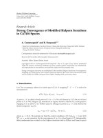
In fact this solution has a very simple interpretation. The
remaining power is waterfilled on top of the existing margin
adaptive waterlevels of the users with non-empty queues. The
additional power is strictly utilized in maximizing the system
throughput without any fear of delay violations. Figure 2
explains the multi-level waterfilling in multiuser OFDMA
system for the feasible case with K = 2 and F = 8. δ1 and δ2
are the margin adaptive waterlevels corresponding to users 1
t
and 2, respectively. For each user, channel gains gk, f on their
allocated subcarriers are inverted which are represented by
the blank regions. The amount of margin adaptive power
allocated on each subcarrier is represented by the shaded
portion and the additional power is waterfilled on top of

margin adaptive water levels. Throughput is maximized
because more power is allocated to the users which can
t+1
achieve maximum data rates. Finally, the backlog values Bk
are updated accordingly for the next time slot. Thus the
additional power is now utilized in strictly increasing the
sum-rate of the system without fearing about the packet
drops and delay violations.


10

EURASIP Journal on Wireless Communications and Networking

4.3. Nonfeasible Case: Pmg > Pmax . In this case, we cannot
respect all the minimum rates proposed by MRS during
current time slot. In order to respect the constraint on
Pmax , we have to decrease the data rates of the users. We
develop an algorithm where the data rates of some of
the users are decreased in such a way that throughput is
least sacrificed. Moreover, we ensure in this algorithm that
minimum number of users are affected by the rate decrease
so that the proposed rates of maximum number of users are
attained. Again we use the subcarrier allocation as obtained
by margin adaptive algorithm. Our algorithm is based on the
observation that MRS propose higher data rates in following
scenarios: (i) user channel is good compared to its mean
channel gain, (ii) backlog value is high, and (iii) both (i) and
(ii). Therefore, the user with maximum data rate constraint
is the user with urgent need of data transmission. Decreasing

its data rate will result in maximum delay violations. Let
t,k
t,k
Rm be the margin adaptive rate and Pm be the margin
adaptive power allocated to user k. We have Algorithm 1 for
the nonfeasible case.
In step 1, we identify a data rate region C. All the users
whose demanded rates lie in this interval are the ones with
urgent need of data rate transmission. In step 2, we form a
set of users which will be considered for possible decrease in
their data rate. We select a user k which consumes maximum
power to achieve its rate constraint. This user represents the
worst user of the set Ω. Therefore, if we decrease its data rate
by a small amount we will end up saving a huge amount
of power. We repeat the process till Pmax is achieved. This
algorithm converges for small values of Δ. In step 1, φ is used
to determine the lower bound on interval C. This parameter
is adjusted in such a way that enough users are included in
the set Ω for possible rate decrease.
Since we have decreased the data rates of some of the
users, their backlog has increased. MRS utilizes the backlog
information in its scheduling decisions hence it will propose
a high data rate for such users in next time slots. Thus such
users will get a higher data rate in future time slots in order
to avoid packet drops, thereby decreasing the overall packet
drop rate.

5. Complexity Analysis
In this section, we will separately analyze the complexity of
the scheduler and the resource allocation algorithms.

5.1. MRS Complexity. The scheduler operates in two parts.
In the first part, the MRS algorithm propose output rates
without the bounding constraints (26) and (27) while in the
second part these rates are adjusted in Case I to Case III. We
separately analyze the complexity of these two parts.
(1) During each time slot, the MRS algorithm has four
steps all of which involve mathematical operations.
Let C1 denote the complexity of the mathematical
operations involved in this algorithm. Since each user
has a separate MRS, the total complexity of this part
is KC1 .

Table 3: Complexity order of different algorithms for K users and
F subcarriers in the system.
Algorithm
Complexity Order Required CSI (tti)
MRS scheduler
O(2K)
1
1
Margin Adaptive Algorithm
O(Im FK)
Feasible case
O(K)
1
1
Nonfeasible case
O(In f FK)

(2) The additional complexity of the scheduler comes

from the second step where the output rates are
adjusted in Case I to Case III. Case I and Case II do
not incur additional complexity. Case III can result
in solving additional optimization problems by using
the MRS algorithm. The maximum complexity of
this step occurs when all the users require Case III.
In this situation, the complexity of this part becomes
equal to that of part 1.
Thus the maximum complexity of scheduling is CS =
2KC1 . Since the complexity of mathematical operations
can be ignored it can be concluded that the maximum
complexity of the scheduler is of the order O(2K).
5.2. Margin Adaptive Algorithm. The complexity of this
algorithm depends on the number of iterations Im required
t
to update the waterlevels δk for a given step size Δm . Since
the algorithm has to find the best user on each subcarrier
by employing waterfilling power allocation, therefore, the
complexity order of the sum-power minimization algorithm
becomes O(Im FK). The complexity of this algorithm is
polynomial in number of users and subcarriers.
5.3. Feasible Case. This algorithm is not an iterative algorithm and like MRS only involves mathematical operations.
Let C2 denote the complexity of the waterfilling operation in
this case. Since additional power is allocated to the users with
non-empty queues on top of the margin adaptive waterlevels,
hence the complexity of this algorithm depends only on the
number of users with non-empty queues. The number of
such users can be less than or equal to the total number of
users in the system. Therefore, the maximum complexity of
this algorithm can be CFC = KC2 and the complexity order

is O(K).
5.4. Nonfeasible Case. The algorithm for the non-feasible
case is an iterative algorithm. The complexity of this
algorithm depends on the number of iterations required to
decrease the data rate of the users for a given step size Δ till
convergence. Since the algorithm achieves the new data rate
by using waterfilling algorithm on the subcarriers allocated
by the margin adaptive algorithm, therefore, the complexity
order of this algorithm is O(In f FK). The complexity of
this algorithm is also polynomial in number of users and
subcarriers.
The complexity orders and the required CSI of these
algorithms are given in Table 3.


EURASIP Journal on Wireless Communications and Networking

11

Initialization: Prem = Pmg − Pmax
While Prem > 0
(1) Rub = max Rt,k , Rlb = Rub − φRub , C = [Rlb , Rub ]
m
(2) Ω = {∀k | 0 < Rt,k < Rlb }
m
t,k
(3) k = maxk∈Ω Pm /Rt,k
m
t+1
t+1,k

(4) Rt,k = Rt,k − Δ, Bnew = Bk + Δ
new
m
t,k is achieved by using step 1 of the margin adaptive algorithm.
(5) Rnew
t
t,k
(6) Pnew is the power allocated to user k by waterfilling over Ik .
t,k
t,k
(7) Prem = Prem − {Pm − Pnew }
t+1
t,k
t,k
t+1,k
(8) Pm = Pnew , Rt,k = Rt,k and Bk = Bnew .
m
new

320
300
280
260
240
220
200
180
160
140
120

Packets with delay violations (%)

Achieved rate (bits/OFDM symbol)

Algorithm 1: Pmg > Pmax .

7
6
5
4
3
2
1
0
1

10

12

14

16
18
20
22
Total power (dbs)

24

26

28

Our algo
Hungarian algo

Figure 3: Total achieved rate versus Pmax for 10 user 24 subcarrier
system. Total demanded rate = 100 bits/OFDM symbol.

6. Numerical Analysis
We consider a single cell downlink OFDMA system with
perfect channel state information and a peak power constraint of 43 dBm. We consider a frequency selective Rayleigh
fading channel with exponential delay profile. Path losses
are calculated according to Cost-Hata Model [28]. The
power spectral density of noise is −174 dBm/Hz. Time is
divided into slots and duration of each time slot is 1 ms. A
given number of packets are generated for each user every
time slot. We assume that all the packets have same delay
constraint and each packet has a size of 1 Kbits. The users are
uniformly distributed in a cell of radius 700 m. Moreover, the
bandwidth of each subcarrier is 375 KHz. The simulations
are carried out for different scenarios. In each scenario,
the distances of the users from BS remain constant which
is a realistic assumption for low-speed mobile users. Each
scenario is simulated for a total of 1000 tti which corresponds
to 1 second of real time. Furthermore, in all the scenarios we
assume that one user is always at a maximum distance from
the BS in order to analyze the performance of our approach

for worst user in the system.
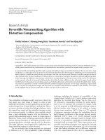
In Figure 3, we compare the performance of our physical
layer algorithm with the algorithm presented in [8] for

1.5

2 2.5 3 3.5 4 4.5 5
Input arrival rate (packets/tti/user)

5.5

6

Delay = 1tti
Delay = 10tti

Figure 4: Percentage of packets with delay violations versus input
arrival rate for all the users in the system. Users = 14, Subcarriers =
40, Cell Radius = 700 m, and tti = 1 ms.

10 users and 24 subcarriers. It should be noted that this
is the comparison of the physical layer resource allocation
algorithms and not the comparison of our whole approach.
Moreover, we have assumed in this simulation that the
queues are backlogged and there are always packets available
for transmission so that we are able to utilize all the available
power. The authors in [8] solve the resource allocation
problem presented in Section 4 for the feasible case by using
hungarian algorithm. Although the authors do not consider
scheduling and delay constraints, however, their algorithm

can be considered to be applicable for feasible case assuming
that the underlying application demands a delay of D = 1
t,k
t
and Rmin = Xk , for all t, k. From the simulations we can
see that the total achieved rate by our approach is much
higher because for the feasible case our algorithm gives
the remaining power by waterfilling while the algorithm
presented in [8] gives all the remaining resources to the user
with highest mean channel gain value.
In order to evaluate the performance of our whole
scheme (scheduling and resource allocation), we plot Figures
4, 5, 6, and 7. ( The optimal solution for this problem
is unknown in the literature. Moreover, the brute force
method is also not applicable to this framework. In the brute


12

EURASIP Journal on Wireless Communications and Networking

Packets with delay violations (%)

Packets with delay violations (%)

20
18
16
14
12

10
8
6
4
2

22
20
18
16
14
12
10
8
6
4
2
0
90

0
1

1.5

2 2.5 3 3.5 4 4.5 5
Input arrival rate (packets/tti/user)

5.5

6

Delay = 1tti
Delay = 2tti

Delay = 1tti
Delay = 10tti

Figure 5: Percentage of packets with delay violations versus input
arrival rate for worst user. Users = 14, Subcarriers = 40, Cell Radius
= 700 m, and tti = 1 ms.

Delay = 5tti
Delay = 10tti

Figure 7: Percentage of packets with delay deadline violations for
worst user versus delay constraint achievement probability. Users =
14, Subcarriers = 40, Input arrival rate = 6 packets/tti, Cell Radius =
700 m, and tti = 1 ms.

8

70

7

Average sum output rate (packets)

Packets with delay violations (%)

91 92 93 94 95 96 97 98 99 100
Delay constraint achievement probability (worst user)

6
5
4
3
2

60
50
40
30
20

1
10
10

0
90

92
94
96
98
100
Delay constraint achievement probability (all users)
Delay = 1tti
Delay = 2tti

Delay = 5tti
Delay = 10tti

Figure 6: Percentage of packets with delay deadline violations for
all user versus delay constraint achievement probability. Users = 14,
Subcarriers = 40, Input arrival rate = 6 packets/tti, Cell Radius =
700 m,and tti = 1 ms.

force method we have to try all the possible combinations.
However, in this case since the rate is given by a continuous
function w.r.t power there are infinite possibilities. It is therefore impossible to obtain the optimal solution using brute
force method. Hence comparisons with optimal solution of
this problem are not possible.) We plot these figures for 14
users and 40 subcarriers. Figure 4 shows the input arrival
rate versus the percentage of packets whose delay constraints
are violated for all the users in the system. We are interested
in the maximum input arrival rate that can result in strict
delay constraint achievement of all the packets in the system.
When D = 1 tti, input arrival rate has to be constrained to

20
30
40
50
60
Average sum input arrival rate (packets/tti)

70

Delay = 1tti
Delay = 10tti

Figure 8: Average output sum rate versus average sum input arrival
rate. Users = 14, Subcarriers = 40, Cell Radius = 700 m, and tti =
1 ms.

4.9 packets/tti/user for 0% packet delay violations. However,
when D = 10 tti, our scheduling policy is able to deliver 5.9
packets/tti/user without any delay violations. This difference
translates into achieving 14 Mbits/s higher transmission rate
while achieving strict delay constraint for all the packets.
As the input arrival rates are further increased, more and
more packets are unable to achieve their delay constraints.
In Figure 5, we plot the same parameters for worst user in
the system.
Since the main objective of this work is a scheduling
policy for delay constraints in the range of 1 < D < ∞
therefore the performance of the scheduler has to be judged
based on the number of packets which cannot achieve their
delay constraints. We divide the total simulation interval into


EURASIP Journal on Wireless Communications and Networking
subintervals of D time slots. The average achieved rate in each
sub-interval should be greater than or equal to the average
input arrival rate if all the packets are delivered successfully.
If the achieved rate in a sub-interval is greater than or equal
to the average input arrival rate, we term it as 100% delay
achievement probability. However, if the achieved rate is,

for example, 0.9 times the average input arrival rate then
this results in 90% delay achievement probability. We plot in
Figures 6 and 7 the delay constraint achievement probability
versus the percentage of packets whose delay constraints are
violated at the input arrival rate of 6 packets/tti/user. The
figures are plotted for different values of delay constraints for
the worst user and for all the users in the system. We can see
that as D increases, more and more packets are able to achieve
their respective delay constraints. In case of worst user when
D = 1, at 100% delay achievement probability almost 80%
of the packets are able to achieve their demanded delay
constraint. However, when D = 10tti, the delay violations are
less than 1% which goes to zero for 90% delay achievement
probability. It is also evident that maximum improvement is
achieved when delay is increased from 1tti to 2tti. In case of
worst user, at 100% delay achievement probability only 6%
of the packets are unable to achieve their delay constraints
when D = 2 compared to more than 19% of the packets
whose delay constraints are violated when D = 1. Therefore,
by allowing a small delay tolerance huge performance gains
can be made.
Finally in Figure 8 we plot the average output sum rate
versus the average sum input arrival rate for D = 1 and D =
10 tti. It should be noted that the achieved data rates are the
same till we reach the average sum input rate of 50 packets/tti.
Since we do not consider infinite backlogged queues in our
analysis and in the context of strict delay constraints, we drop
the packets whose delay deadlines are not achieved thus all we
can do is to transmit all the available packets in these queues.
However, it is obvious that for lower values of sum input

arrival rates there is some power available which is wasted if
the user queues are empty and there are no more packets left
for transmission. As the sum input arrival rate increase, we
can transmit more packets till we reach the point where delay
deadlines of the packets start getting violated. If we further
increase the sum input arrival rate beyond this point the
achieved sum rate becomes a flat curve since system capacity
is reached and we cannot transmit more packets. However,
for D = 10 tti the curve gets flat at input sum arrival rate of
60 packets/tti compared to 50 packets/tti for D = 1 tti.

7. Conclusion
In this paper, we have given a two-step solution to the
sum-rate maximization problem with strict delay constraints
on data transmission in OFDMA system. In the first step,
we developed a causal Minimum Rate Scheduler for packet
delays in the range of 1 < D < ∞. The proposed data rates
by the scheduler conceals the delay constraints from physical
layer resource allocation block. Based on the minimum data
rates and limited power budget, we studied the feasibility
conditions of our resource allocation problem. We developed

13

efficient algorithms for the feasible and the non-feasible
cases. By separating scheduling from resource allocation, we
achieved a significant reduction in complexity by solving a
series of simple optimization problems. Simulation results
revealed that by increasing packet delay constraint higher
input arrival rates can be supported. The enhanced performance at higher values of delay constraint is due to better

exploitation of time, frequency, and multiuser diversities.

References
[1] B. Yang, K. B. Letaief, R. S. Cheng, and Z. Cao, “Channel estimation for OFDM transmission in multipath fading channels
based on parametric channel modeling,” IEEE Transactions on
Communications, vol. 49, no. 3, pp. 467–479, 2001.
[2] C. Y. Wong, R. S. Cheng, K. B. Letaief, and R. D. Murch,
“Multiuser OFDM with adaptive subcarrier, bit, and power
allocation,” IEEE Journal on Selected Areas in Communications,
vol. 17, no. 10, pp. 1747–1758, 1999.
[3] J. Jang and K. B. Lee, “Transmit power adaptation for
multiuser OFDM systems,” IEEE Journal on Selected Areas in
Communications, vol. 21, no. 2, pp. 171–178, 2003.
[4] W. Rhee and J. M. Cioffi, “Increase in capacity of multiuser
OFDM system using dynamic subchannel allocation,” in
Proceedings of the Vehicular Technology Conference (VTC ’00),
vol. 2, pp. 1085–1089, May 2000.
[5] D. N. C. Tse and S. V. Hanly, “Multiaccess fading channelspart I: polymatroid structure, optimal resource allocation
and throughput capacities,” IEEE Transactions on Information
Theory, vol. 44, no. 7, pp. 2796–2815, 1998.
[6] R. Knopp and P. A. Humblet, “Information capacity and
power control in single-cell multiuser communications,” in
Proceedings of the IEEE International Conference on Communications, vol. 1, pp. 331–335, June 1995.
[7] G. Caire, G. Taricco, and E. Biglieri, “Optimum power control
over fading channels,” IEEE Transactions on Information
Theory, vol. 45, no. 5, pp. 1468–1489, 1999.
[8] H. Yin and H. Liu, “An efficient multiuser loading algorithm
for OFDM-based broadband wireless systems,” in Proceedings
of the IEEE Global Telecommunication Conference (GLOBECOM ’00), vol. 1, pp. 103–107, December 2000.
[9] D. Niyato and E. Hossain, “Adaptive fair subcarrier/rate

allocation in multirate OFDMA networks: radio link level
queuing performance analysis,” IEEE Transactions on Vehicular
Technology, vol. 55, no. 6, pp. 1897–1907, 2006.
[10] B. Bai, W. Chen, Z. Cao, and K. B. Letaief, “Achieving high
frequency diversity with subcarrier allocation in OFDMA
systems,” in Proceedings of the IEEE Global Telecommunications
Conference (GLOBECOM ’08), pp. 1–5, November 2008.
[11] P. Viswanath, D. N. C. Tse, and R. Laroia, “Opportunistic
beamforming using dumb antennas,” IEEE Transactions on
Information Theory, vol. 48, no. 6, pp. 1277–1294, 2002.
[12] Y. Liu and E. Knightly, “Opportunistic fair scheduling over
multiple wireless channels,” in Proceedings of the 22nd Annual
Joint Conference on the IEEE Computer and Communications
Societies (INFOCOM ’03), vol. 2, pp. 1106–1115, March 2003.
[13] G. Song, Y. Li, L. J. Cimini Jr., and H. Zheng, “Joint
channel-aware and queue-aware data scheduling in multiple
shared wireless channels,” in Proceedings of the IEEE Wireless
Communications and Networking Conference (WCNC ’04), vol.
3, pp. 1939–1944, March 2004.
[14] M. Andrews, K. Kumaran, K. Ramanan, A. Stolyar, R.
Vijayakumar, and P. Whiting, “CDMA data QoS scheduling on


14

[15]

[16]

[17]

[18]

[19]

[20]

[21]

[22]

[23]

[24]
[25]

[26]

[27]

[28]

EURASIP Journal on Wireless Communications and Networking
the forward link with variable channel conditions,” Technical
Memo, Bell Labs, April 2000.
S. Shakkottai and A. L. Stolyar, “Scheduling for multiple flows
sharing a time-varying channel: the exponential rule,” Analytic
Methods in Applied Probability, vol. 207, pp. 185–202, 2002.
G. Song and Y. Li, “Utility based resource allocation and
scheduling in OFDM based wireless broadband networks,”

IEEE Transactions on Wireless Communications, vol. 43, pp.
127–134, 2005.
H. T. Cheng and W. Zhuang, “Joint power-frequency-time
resource allocation in clustered wireless mesh networks,” IEEE
Transactions on Networks, vol. 22, no. 1, pp. 45–51, 2008.
C. Zhou and G. Wunder, “A novel low delay scheduling
algorithm for OFDM broadcast channel,” in Proceedings of
the 50th Annual IEEE Global Telecommunications Conference
(GLOBECOM ’07), pp. 3709–3713, November 2007.
M. A. Khojastepour and A. Sabharwal, “Delay-constrained
scheduling: power efficiency, filter design, and bounds,” in
Proceedings of the IEEE Conference on Computer Communications (INFOCOM ’04), pp. 1938–1949, March 2004.
R. A. Berry and R. G. Gallager, “Communication over
fading channels with delay constraints,” IEEE Transactions on
Information Theory, vol. 48, no. 5, pp. 1135–1149, 2002.
B. Collins and R. L. Cruz, “Transmission policies for time
varying channels with average delay constraints,” in Proceedings of the 37th Annual Allerton Conference on Communication,
Control and Computing, September 1999.
D. Rajan, A. Sabharwal, and B. Aazhang, “Delay-bounded
packet scheduling of bursty traffic over wireless channels,”
IEEE Transactions on Information Theory, vol. 50, no. 1, pp.
125–144, 2004.
W. Chen, M. J. Neely, and U. Mitra, “Energy efficient scheduling with individual packet delay constraints: offline and online
results,” in Proceedings of the IEEE 26th IEEE International
Conference on Computer Communications (INFOCOM ’07),
pp. 1136–1144, May 2007.
S. Boyd and L. Vandenberghe, Convex Optimization, Cambridge University Press, Cambridge, UK, 2003.
D. P. Palomar and M. Chiang, “A tutorial on decomposition
methods for network utility maximization,” IEEE Journal on
Selected Areas in Communications, vol. 24, no. 8, pp. 1439–

1451, 2006.
A. G. Marques, X. Wang, and G. B. Giannakis, “Dynamic
resource management for cognitive radios using limited-rate
feedback,” IEEE Transactions on Signal Processing, vol. 57, no.
9, pp. 3651–3666, 2009.
A. G. Marques, G. B. Giannakis, F. F. Dignam, and F. J.
Ramos, “Power-efficient wireless OFDMA using limited-rate
feedback,” IEEE Transactions on Wireless Communications, vol.
7, no. 2, pp. 685–696, 2008.
Cost 231, “Urban transmission loss models for mobile radio
in the 900 and 1800 MHz bands,” Tech. Rep. TD (90) 119 Rev
2, September 1991.