Báo cáo hóa học: " Research Article Opportunistic Adaptive Transmission for Network Coding Using Nonbinary LDPC Codes" pptx

Hindawi Publishing Corporation
EURASIP Journal on Wireless Communications and Networking
Volume 2010, Article ID 517921, 15 pages
doi:10.1155/2010/517921

Research Article
Opportunistic Adaptive Transmission for
Network Coding Using Nonbinary LDPC Codes
Giuseppe Cocco, Stephan Pfletschinger, Monica Navarro, and Christian Ibars
Centre Tecnol`gic de Telecomunicacions de Catalunya, 08860 Castelldefels, Spain
o
Correspondence should be addressed to Giuseppe Cocco,
Received 31 December 2009; Revised 14 May 2010; Accepted 3 July 2010
Academic Editor: Wen Chen
Copyright © 2010 Giuseppe Cocco et al. This is an open access article distributed under the Creative Commons Attribution
License, which permits unrestricted use, distribution, and reproduction in any medium, provided the original work is properly
cited.
Network coding allows to exploit spatial diversity naturally present in mobile wireless networks and can be seen as an example
of cooperative communication at the link layer and above. Such promising technique needs to rely on a suitable physical layer in
order to achieve its best performance. In this paper, we present an opportunistic packet scheduling method based on physical layer
considerations. We extend channel adaptation proposed for the broadcast phase of asymmetric two-way bidirectional relaying to
a generic number M of sinks and apply it to a network context. The method consists of adapting the information rate for each
receiving node according to its channel status and independently of the other nodes. In this way, a higher network throughput
can be achieved at the expense of a slightly higher complexity at the transmitter. This configuration allows to perform rate
adaptation while fully preserving the benefits of channel and network coding. We carry out an information theoretical analysis
of such approach and of that typically used in network coding. Numerical results based on nonbinary LDPC codes confirm the
effectiveness of our approach with respect to previously proposed opportunistic scheduling techniques.

1. Introduction
Intensive work has been devoted the field of network coding
(NC) since the new class of problems called “network

information flow” was introduced in the paper of Ahlswede
et al. [1], in which the coding rate region of a single
source multicast communication across a multihop network
was determined and it was shown how message mixing at
intermediate nodes (routers) allows to achieve such capacity.
Linear network coding consists of linearly combining packets
at intermediate nodes and, among other advantages [2],
allows to increase the overall network throughput. In [3],
NC is seen as an extension of the channel coding approach
introduced by Shannon in [4] to the higher layers of the
open systems interconnection (OSI) model of network architecture. Important theoretical results have been produced in
the context of NC such as the min-cut max-flow theorem
[5], through which an upper bound to network capacity can
be determined, or the technique of random linear network
coding [6, 7] that achieves the packet-level capacity for
both single unicast and single multicast connections in both

wired and wireless networks [3]. Practical implementations
of systems where network coding is adopted have also been
proposed, such as CodeCast in [8] and COPE in [9].
The implementation proposed in [9] is based on the idea
of “opportunistic wireless network coding”. In such scheme
at each hop, the source chooses packets to be combined
together so that each of the sinks knows all but one of the
packets. Considering the problem in a wireless multihop
scenario, each of the potential receivers will experiment
different channel conditions due to fading and different
path losses. At this point, a scheduling problem arises:
which packets must be combined and transmitted? Several
solutions to this scheduling problem have been proposed up

to now. In [10], a solution based on information theoretical
considerations is described, that consists of combining and
transmitting, with a fixed rate, packets belonging only to
nodes with highest channel capacities. The number of such
nodes is chosen so as to maximize system throughput.
In [11], the solution [10] has been adapted to a more
practical scenario with given modulations and finite packet
loss probabilities. In both cases network coding and channel


2

EURASIP Journal on Wireless Communications and Networking

coding are treated separately. However, as pointed out in the
paper by Effros et al. [12], such approach is not optimal
in real scenarios. In [13, 14], a joint network and channel
coding approach has been adopted to improve transmissions
in the two-way relay channel (TWRC) in which two nodes
communicate with the help of a relay. One of the main ideas
used in these works is that of applying network coding after
channel encoding. This introduces a new degree of flexibility
in channel adaptation, which leads to a decrease in the packet
error rate of both receivers.
Up to our knowledge, this approach has been applied
only to the two-way relay channel. In the present paper,
we extend the basic idea of inverting channel and network
coding to a network context. While in the TWRC the
relay broadcasts combinations of messages received by the
two nodes willing to communicate, in our setup the relay

can have stored packets during previous transmissions by
other nodes, which is typical in a multihop network, and
transmit them to a set of M sinks. As a matter of fact,
in a wireless multihop network more than just two nodes
(sinks) are likely to overhear a given transmission. Due to the
different channel conditions, a per-sink channel adaptation
is done in order to enhance link reliability and decrease
frequent retransmissions which can congest parts of the
network, especially when ARQ mechanisms are used [9]. In
particular, packet ui of length K is considered as a buffer by
the transmitting node (source node). At each transmission,
a part of the buffer, containing K bits, is included in a
new packet of total length N that contains N − K bits of
redundancy. Network Coding combination takes place on
such packets. The value of K , which determines the amount
of redundancy to be introduced in each combined packet
(i.e., the code rate), is chosen by the source node considering
the physical channel between source node and sink i. Given
a set of channel code rates {r1 , . . . , rs }, we propose that the
code rate in channel i be the one that maximizes the effective
throughput on link i defined as
thi = rk 1 − ppli (rk ) ,

(1)

where ppli (rk ) is the current probability of packet loss on
channel i when using rate rk .
In present paper, we carry out an information theoretical
analysis and comparison for the proposed method and the
method in [10], which maximizes overall throughput in a

system where opportunistic network coding is used, showing
how the first one noticeably enhances system throughput.
Moreover, we evaluate the performance of the two methods
in a real system using capacity-approaching nonbinary lowdensity parity-check (LDPC) codes at various rates (in [13,
14] parallel concatenated convolutional codes (PCCC) have
been adopted for channel coding). Numerical results confirm
those obtained analytically. Finally, we consider some issues
regarding how modifications at physical level affect network
coding from a network perspective.
The paper is organized as follows. In Section 2, the system
model is described. In Section 3, we propose a benchmark
system with equal rate link adaptation. Section 4 contains
the description of our proposed opportunistic adaptive

transmission for network coding. In Section 5, we carry out
the comparison between the two methods by comparing
the cumulative density functions of the throughput and the
ergodic achievable rates. Section 6 contains the description of
the simulation setup and the numerical results. In Section 7,
we consider some scheduling and implementation issues at
network level that arise from applying the proposed adaptive
transmission method, and finally in Section 8, we draw the
conclusions about the results obtained in this paper, and we
suggest possible future work to be carried out.

2. System Model
2.1. Network Level. Let us consider a mobile wireless multihop network such as the one depicted in Figure 1. We denote
by Fq the finite field (Galois field) of order q = 2l . Each
packet is an element in FK ; that is, it is a K-dimensional
q

vector with components in Fq . We say that a node ni is the
generator of a packet pi if the packet pi originated in ni . We
say that a node is the source node during a transmission slot
if it is the node which is transmitting. We call sink node the
receiving node during a given transmission slot and destination node the node to which a given packet is addressed.
We will refer to generators’ packets as native packets. Each
node stores overheard packets. Native and overheard packets
are transmitted to neighbor nodes. For ease of exposition
and without loss of generality we assume that a collision-free
time division multiple access is in place. The number of hops
needed to transmit a packet from generator to destination
node depends on the relative position of the two nodes in
the network. In Figure 1, two generator-destination pairs
are shown (G1–D1, G2–D2). Thin dashed lines in the figure
represent wireless connectivity between nodes and thick lines
represent packet transmissions. G1 has a packet to deliver to
D1 and G2 has a packet to deliver to node D2. In the first time
slot, generator G1 and G2 broadcast their packets p1 and p2,
respectively, (thick red dash-dotted line). In the second time
slot, node 6 acts as a source node broadcasting packet p2
(thick green dotted line) received in previous slot. Note that
in this case node 6 is a source node but not a generator node.
Finally, in the third time slot, node 5 broadcasts the linear
combination in a finite field of packets p1 and p2 (indicated
in Figure 1 with p1 + p2). Destination nodes D1 and D2 can,
respectively, obtain packets p1 and p2 from p1 + p2 using
their knowledge about packets p2 and p1 overheard during
previous transmissions.
In general, using linear network coding we proceed
as follows. Each node stores overheard packets, linearly

combines them and transmits the combination together with
the combination coefficients. As the combination is linear
and coefficients are known, a node can decode all packets
if and only if it receives a sufficient number of linearly
independent combinations of the same packets. At this point,
a scheduling solution must be found in order to decide which
packets must be combined and transmitted each time. In the
paper by Katti et al. [9], a packet scheduling based on the
concept of network group has been described. Such solution,
called opportunistic coding, consists of choosing packets so
that each neighbor node knows all but one of the encoded


EURASIP Journal on Wireless Communications and Networking

3

Node 3
(G2)

Node 2
(D1)

Node 1

p1 + p2

p2

p2

p1 + p2

p2

p2
p1 + p2
Node 4
(D2)

p2

Node 5
p1

p2

Node 6

p1 + p2

p2
Node 7

p1
p1 + p2

Node 8
(G1)

p1
p1

Node 10

p1 + p2

p1 + p2
Node 9

Node 14

Node 13
Node 12
Node 11

1st time slot
2nd time slot
3rd time slot

Figure 1: Mobile wireless multihop network. Two different information flows exist between two generator-destination pairs G1–D1 and
G2–D2. Thin dashed lines represent wireless connectivity among nodes while thick lines represent packet transmissions. In the first time slot
generator G1 and G2 broadcast their packets p1 and p2, respectively, (thick dash-dotted line). In the second time slot, node 6 broadcasts
packet p2 (thick dotted line) received in previous slot. In the third time slot, node 5 broadcasts the linear combination of packets p1 and p2
(p1 + p2). Destination nodes D1 and D2 can, respectively, obtain packets p1 and p2 from p1 + p2 using their knowledge about packets p2
and p1 overheard during previous transmissions.

packets. Such approach has been implemented in the COPE
protocol, and its practical feasibility has been shown in [9].
A network group is formally defined as follows.

Definition 1. A set of nodes is called a size M network group
(NG) if it satisfies the following:
(1) one of the nodes (source) has a set U = {u1 , . . . , uM }
of M native packets to be delivered to the other nodes
in the set (sinks);
(2) all sink nodes are within the transmission range of
the source;
(3) each of the sink nodes has all packets in U but
one (they may have received them during previous
transmissions).
All native packets are assumed to contain the same number K
of symbols. A native packet is considered as a K-dimensional
vector with components in Fq with q = 2l , that is, a native
packet is an element in FK .
q
Figure 2 shows an example of how a network group is
formed during a transmission slot.

Network groups appear in practical situations in wireless
mesh networks and other systems. A classical example is a
bidirectional link where two nodes communicate through a
relay. More examples can be found in [9]. In the following,
we will assume that all transmissions adopt the network
group approach; that is, during each transmission slot, the
source node chooses the packets to be combined so that each
of the sinks knows all but one of the packets. As a matter of
fact, if nodes are close one to each other it is highly probable
that many of them overhear the same packets. Nevertheless
this assumption is not necessary to obtain NC gain or to
apply the technique proposed in this paper. In Section 7, we

will extend the results to a more general case, in which a node
may not know more than one of the source packets.
We assume time is divided into transmission slots. During each transmission slot source node combines together
the M packets in U and broadcasts the resulting packet to
sink nodes of the network group. Let us indicate with ui the
packet to be delivered to node i. The packet transmitted by
the source node is
M

x=

ui ,
i=1

(2)


4

EURASIP Journal on Wireless Communications and Networking

N2
P1

N1

P1

P4

exponentially distributed random variable with probability
density function

P3

1
p γi (t) = e−γi (t)/γ ,
γ

γ2
γ1
N4
(S)

P1

P2

P3

for γi (t) ≥ 0,

(5)

where γ is the mean value of the SNR. We assume that
α
the quantities γi (t)dsi at the various sinks are i.i.d. random
variables. In the model we are not taking into account
shadowing effects.

P4

γ3

3. Constant Information Rate Opportunistic
Scheduling Solutions

⎛ ⎞

γ1

⎜ ⎟
γ = ⎜γ2⎟
⎝ ⎠

γ3

P3

N3

P4

Figure 2: Network group formation. N4 is going to access the
channel. Node N4 knows which packets are stored in its neighbors’
buffers. Based on this knowledge it must choose which packets to
XOR together in order to maximize the number of packets decoded
in the transmission slot. A possible choice is, for example, P1 + P2
which allows nodes N1 and N2 to decode, but not N3. A better
choice is to encode P1 + P3 + P4, so that 3 packets can be decoded

in a single transmission. The difference in SNR for the three sinks
(γ1 ,γ2 , and γ3 ) can lead to high packet loss probability on some of
the links if a single channel rate is used for all the sinks. γ is the
vector of SNRs.

where indicates the sum in FK . Let us define packet x\ j as
q
follows:
M

x\ j =

ui

(3)

i=1,i = j
/

Sink i can obtain ui by adding x and x\ j in FK , where x\ j is
q
known according to our assumptions.
Note that in the network in Figure 1 many aspects deserve
in-depth study, such as end-to-end scheduling of packet
transmissions on multiple access schemes. These aspects are
however beyond the scope of this paper, where we focus on
maximizing the efficiency of transmissions within a network
group.

Based on the propagation model in (5), the channel from

source to each sink will have a different gain. The difference
in link states experienced by the sinks gives rise to the
problem of how to choose the broadcast transmission rate.
In [10], an interesting solution has been proposed based
on information-theoretical capacity considerations. Sink
nodes are ordered from 1 to M with increasing SNR. The
solution proposed consists of combining and transmitting
only packets having as destination the M − v + 1 sinks with
highest SNR. The transmission rate R chosen by the source
node is the lowest capacity in the group of M − v + 1
channels. The instantaneous capacity obtained during each
transmission is then
(v)
Cinst = (M − v + 1)log2 1 + γ(v) ,

where γ(v) is the SNR experienced on the vth worse channel.
v is chosen so that (6) is maximized. Note that all sinks in
the network group receive the same amount of information
per packet. In [11], another approach is proposed in which
the source node transmits to all nodes in the NG. A practical
transmission scheme with finite bit error probability and
fixed modulations is described.
3.1. Constant Information Rate Benchmark. Based on [10,
11], we define a constant information rate (CIR) system that
will be used as a benchmark to our proposed adaptive system.
Let us now define the effective throughput as
M

2.2. Physical Level. Physical links between source and sinks
are modeled as frequency-flat, slowly time-variant (block

fading) channels. The SNR of sink i during time slot t can
be expressed as
γi (t) =

Ptx |hi (t)|2
,
α
dsi σ 2

(4)

where Ptx is the power used by source node during transmission, hi (t) is a Rayleigh distributed random variable that
models the fading, dsi is the distance between source and
sink i, α is the path loss exponent and σ 2 is the variance
of the AWGN at sink nodes. From expression (4) it can
be seen that the SNR at a receiver with a given dsi is an

(6)

th =

1 − ppli ri = 1 − ppl

T

r,

(7)

i=1

where ppl and r are two M ×1 vectors containing, respectively,
the packet loss probabilities and the coding rates for the
various links, T represents the transpose operator and 1 is
an M-dimensional vector of all ones. The quantity expressed
in (7) measures the average information flow (bits/sec/Hz)
from source to sinks. ppl is an M-dimensional function that
depends on the modulation scheme, coding rate vector r and
SNR vector γ. We assume channel state information (CSI) at
both transmitter and receiver (i.e., the source knows vector γ
containing the SNR of all sinks and node i knows γi ).
In the CIR system, the source calculates first the rate
of the channel encoder which maximizes the effective


EURASIP Journal on Wireless Communications and Networking
throughput for each sink (individual effective throughput).
Formally, for each sink i, we calculate
ri∗ = arg max 1 − ppli γi , ri ri ,

(8)

ri

where ppli (γi , ri ) is the packet loss probability on the ith link
∗
depending on the rate ri . For each rate rk , we define mk as
the number of sinks for which
∗
ri ≥ rk .

(9)

At this point, for each k we calculate the effective throughput,
setting r = r k 1k where 1k is a mk -dimensional vector of
all ones. Finally, we choose k to maximize the effective
throughput. Note that with the CIR approach only sinks
whose optimal rate is greater or equal than the rate which
maximizes the total effective throughput will receive data.

5

As previously stated we will assume that a constant
energy per channel symbol is used. We will not consider
the case of constant energy per information bit as packet
combination at source node is done in FK before channel
q
symbol amplification.
As we will see in Section 6, in this paper, we consider
nonbinary LDPC codes which have a word error rate
characteristic (WER) versus SNR with a high slope. Thus,
the packet loss probability is negligible (≤10−3 ) beyond a
given SNR threshold and rapidly rises below the threshold.
The threshold depends of the code rate considered. Under
this assumption, (10) can be approximated with
⎛

ropt γ = arg max⎝
r

= arg max
r

4. Opportunistic Adaptive Transmission for
Network Coding
We propose a scheme in which information rate is adapted to
each sink’s channel. This can be accomplished by inverting
the order of channel coding and network coding at the
source. In order to explain our method, let us consider again
Figure 2. In the figure, a network group is depicted, in which
node 4 accesses the channel as source node (S) and nodes N1,
N2 and N3 are the sink nodes.
As mentioned in Section 2, the source is assumed to know
the packets in each sink (this can be accomplished with a
suitable ACK mechanism such as the one described in [9]).
We propose a transmission scheme for a size M Network
Group consisting in M variable-rate channel encoders, a FK
q
adder and a modulator as shown in Figure 3. We assume
CSI at both ends. The transmission scheme is as follows.
Based on the SNR to sink i, γi , the source chooses the code
rate ri = Ki /N that maximizes the throughput to sink i,
i = 1, . . . , M. Overall, the rate vector chosen by the source
is the one that maximizes the effective throughput, defined
as
⎛

ropt γ = arg max⎝
r

= arg max
r

M

⎞

1 − ppli γi , ri ri ⎠

i=1

1 − ppl γ, r

(10)
T

r .

As we are under the hypothesis of independent channel gains,
optimal rate can be found independently for each physical
link. In order to apply our method to a packet network, we fix
the size of coded packets to N symbols. Channel adaptation is
performed by varying the number of information symbols in
the coded packet. So, referring to Figure 3, once the optimal
rate ri∗ = Ki /N has been chosen for link i, i = 1, . . . , M, the
source takes Ki information symbols from native packet ui
and encodes them with a rate ri∗ encoder, thus obtaining a
packet ui of exactly N symbols. Finally, packets u1 , . . . , uM
are added in Fq , modulated and transmitted. On the receiver
side, sink i is assumed to know a priori the rate used by the

source for packet ui as it can be estimated using CSI.

M
i=1

⎞

1 − ppli γi , ri ri ⎠

1 − ppl γ, r

(11)
T

r ,

where ppli (γi , ri ) takes value 1 if γ ≤ γthresh and 0 otherwise,
γthresh being a threshold that depends on the rate ri . We will
refer to our approach as adaptive information rate (AIR),
indicating that the number of information bits per packet
received by a given sink is adapted to its channel status. The
same approximation regarding ppl will be used for the CIR
system.

5. Information Theoretical Analysis
Let us consider a system where opportunistic network coding
[9] is used. As described in Section 2, opportunistic Network
Coding consists in a source node combining together and
transmitting M native packets to M sinks. Each of the
sinks knows a priori all but one of the native packets (see

Figure 2). Each of the receivers can, then, remove such
known packets in order to obtain the unknown one. In
the following, we provide an outline of the achievability
for the achievable rate of the system, based on the results
in [15] for the broadcast channel with side information
[16]. In order to study the proposed adaptive transmission
method we need to introduce an equivalent theoretical
model. We model each of the M packets stored in the
source node as an information source. Thus an equivalent
model for our system is given by a scheme with a set of
M information sources IS = {IS1 , . . . , ISM } all located in
the source node, and a set of M sinks D = {D1 , . . . , DM }.
Information source ISi produces a message addressed to sink
Di who has side information (perfect knowledge, specifically)
about messages produced by sources in the subset IS \
ISi . This models the situation in which each of the sinks
knows all but one of the messages transmitted by source
node (see Figure 2). Figure 4 depicts the equivalent model.
Let us consider the system we described in Section 4.
The theoretical idea behind such system is to adapt the
information rate of each information source ISi to channel
i. Each information source ISi chooses a message from a set
of 2nRi different messages. An M-dimensional channel code
book is randomly created according to a distribution p(x)
and revealed to both sender and receiver. The number of


6

EURASIP Journal on Wireless Communications and Networking

Source node

U1

K1 Multiple rate LDPC
encoder for sink 1

U2

K2 Multiple rate LDPC
encoder for sink 2

Network group
(M sinks)

Channel 1

Channel 2

Channel M

.
.

.
.
.
N

Modulo

2 adder

Source buffer

Sink M

.
.

Modulator

KM Multiple rate LDPC
encoder for sink M

UM

Sink 2

N

N
.
.
.

Sink 1

CSI for all sinks(γ vector)

Figure 3: Transmission scheme at source node for the proposed adaptive transmission scheme: the number of information symbols per

packet addressed to a given sink is adapted to the sink’s channel status using channel encoders at different rates. In the picture, the packet
length at the output of the various blocks is indicated.

M

sequences in the channel code book is 2n i=1 Ri . Source node
produces a set of M messages, one for each information
source in it. Given a set of messages, the corresponding
channel codeword X is selected and transmitted over the
channel. Sink Di decodes the output Yi of his channel by
fixing M − 1 dimensions in the channel code book using
its side information about the set of information sources
S \ ISi and applying typical set decoding along dimension i. If
we impose that for each information source Ri < I(X ; Yi ) =
log2 (1 + γi ) where X and Yi are, respectively, the input
and output of a channel where only transmission to sink
Di takes place, then an achievable rate for the system is the
sum of the instantaneous achievable rates of the various
links
M

Rair =
v=1

log2 1 + γv .

that produce messages addressed to these nodes are selected
for transmission. An achievable rate for this system can be
obtained from (12) by setting to 0 the first v terms in the
sum, setting the others equal to log2 (1 + γv ) and optimizing

with respect to v
Rcir = max (M − v + 1)log2 1 + γ(v)
v

,

(13)

where γ(v) indicates the vth worst channel SNR. In order
to compare the two approaches, we will consider the
probability, or equivalently the percentage of time, during
which each of the systems achieves a rate lower than a given
value R, that is,

(12)

Let us now consider the scheduling solution proposed
in [10]. According to this solution, sinks are ordered from
1 to M with increasing channel quality. The M − v + 1
information sources aiming to transmit to the M − v + 1
sinks with best channels (i.e., sinks Dv , Dv+1 , . . . , DM ) are
selected. Each information source in the source node chooses
a message from a set of 2nR elements, where R is chosen so
that R = log2 (1 + γv ). This means that only sinks whose
channels have instantaneous capacity greater than or equal to
node v can decode their message. Only information sources

P {Rinst < R} = FRinst (R),

(14)

where FRinst (R) is the cumulative density function of the
variable Rinst . In the constant information rate system such
probability is

P {Rcir < R} = P max (M − v + 1)log2 1 + γv
v

(15)


EURASIP Journal on Wireless Communications and Networking

7
{W2 , . . . , WM }

Channel 1
p (y1 |x)

IS-1

Y1

W1

Decoder 1
{ W1 , W 3 , . . . , W M }

W1

Y2

IS-2
X

M-dimensional
encoder

W2

W2

Channel 2
p (y2 |x)

.
.
.

Decoder 2
.
.
.

.
.
.

{W1 , W2 , . . . , WM −1 }

WM
IS-M

Channel M
p (yM |x)

YM

WM

Decoder M

Source node
Sink nodes

Figure 4: Equivalent scheme for adaptive transmission. M information sources {IS1 , . . . , ISM } are located in the source node. Information
source ISi produces a message addressed to sink i which has previous knowledge of messages produced by information sources in the subset
S \ ISi . p(yi | x) represents the probability transition function of the channel between the source node and sink i.

We calculated this expression for a network with a generic
number M of nodes (see Appendix A). Such expression is
given by

Let us now consider the cumulative density function
for our proposed system (adaptive information rate). By
definition we have
⎧
⎨M

P {Rair < R} = P ⎩

FRcir (R)
1 M − j1 min(2− j1 ,M − j1 − jM ) min(2− j1 − j2 ,M − j1 − j2 − jM )

=

=P
j1 =0 jM =1

j2 =0

j3 =0

v=1

⎧
⎨M
⎩

v=1

⎫
⎬

log2 1 + γv < R⎭
⎫
⎬

ci < R⎭ =

R
−∞

fc1 (c) ⊗ · · · ⊗ fcM (c)dc,
(19)

min(M −2− j1 −···− jM −3 ,M − j1 − j2 −···− jM −3 − jM )

···

where:
jM −2 =0

×

M!
j1 ! · · · jM !

j

j

j

M − j − j2 −···− jM −2 − jM

M−
α11 α22 · · · αM −22 αM −11

j

M
αM ,

(16)
where
α j = α j (R) = e1/γ e−2

R/( j+1) /γ

− e−2

R/ j /γ

,

(17)

for v = M, and
/
αM = αM (R) = e1/γ e−1/γ − e−2

R/M /γ

,

(18)

γ being the mean value of the SNR, assumed to be exponentially distributed.

fci (c) =

e1/γ
c
ln(2)2c e−2 /γ u(c),
γ

(20)

u(c) being a function that assumes value 0 for c < 0 and 1 for
c > 0. Expression (19) is difficult to calculate in closed form
for the general case. For the low SNR regime we calculated
the following expression (see Appendix B):
P {Rair < R} = 1 − e−R ln(2)/γ

M −1
v=0

v

R ln(2)/γ
.
v!

(21)

In Figure 5, expressions (16) and (21) are compared for
a Network Group of 5 nodes and an average SNR of −10 dB.
The Montecarlo simulation of our system is also plotted for
comparison with (21). At higher SNR (see Figure 6), the CDF

of AIR system is upper bounded by (16) and loosely lower
bounded by the (21) (see Appendix B). A better lower bound
is given by (see Appendix B):
−
FRdir (R) = eM/γ e−1/γ − e−2

R/M /γ

M

.

(22)


8

EURASIP Journal on Wireless Communications and Networking
1
Ergodic achievable rate

0.9
0.8
0.7
CDF

0.6
0.5
0.4
0.3

0.2

10
9
8
7
6
5
4
3
2
1
0

1

1.5

2

2.5

0

0

0.1

0.2

0.3

0.4

0.5

0.6

0.7

0.8

0.9

1

Capacity

Figure 5: Comparison between cumulative density functions in the
system with constant information rate (CIR), adaptive information
rate (AIR) and Montecarlo simulation of AIR. For each value of
R, the constant rate system has a probability not to achieve a rate
equal or greater that R which is higher with respect to our system.
Equivalently, our system will be transmitting at a rate higher than R
for a greater percentage of time.

CDF N =5

3.5

4

4.5

5

Analytical AIR
Montecarlo CIR

Figure 7: Ergodic achievable rate for AIR and CIR systems for
a Network Coding group with M = 5 nodes. The high values of
the rates are due to NC gain. We see how AIR system gains about
2 bits/sec/Hz in all the considered SNR range.

Analytic approximation AIR
Montecarlo AIR
Analytic CIR

1
0.9
0.8
0.7
0.6
0.5
0.4
0.3
0.2
0.1
0

3

Average SNR (dB)

0.1

As for the system with adaptive information rate, we have
⎧
⎨M

Rair = E{Rair } = E⎩

v=1

⎫
⎬

ci ⎭ = ME{ci } = M

1
e1/γ
E1
ln 2
γ

,
(24)

where E1 (x) is the exponential integral defined as
E1 (x) =

∞

1

e−tx
dt.
t

(25)

In Figure 7, the average achievable rate of the two
systems, assuming constant transmitted power, is plotted
against the mean SNR for AIR and CIR systems with M = 5
nodes.

6. Simulation Setup and Results
0

5

10

15

Achievable rate
Analytic AIR (approx. at low SNR)
Montecarlo AIR

Analytic CIR

Lower bound AIR

Figure 6: Comparison between cumulative density functions of the
two systems with M = 5 nodes and SNR = 5 dB. We can see how
for the 40% of time the rate of AIR system will be above 8 bits/s/Hz
while CIR system achievable rate will be above 5.2 bits/s/Hz. At high
SNR the (21) is a loose upper bound for the (19). A tighter lower
bound is given by 22 which is also plotted.

The ergodic achievable rate of the two systems can now
be calculated. For the constant information rate system, we
have
Rcir = E{Rcir } =
where FRcir (c) is given by (16).

+∞
−∞

c

dFRcir (c)
dc,
dc

In this section, we describe the implementation of the
proposed scheme using nonbinary LDPC codes and soft
decoding.
6.1. Notation. During each transmission slot the source node
combines together the packets in U (see Section 4) and
broadcasts the resulting packet to sink nodes of the network

group. In this paper, we used the DaVinci codes, that is, the
nonbinary LDPC codes from the DaVinci project [17]. For
such codes the order of the Galois field is q = 64 = 26 ,
that is, each GF symbol corresponds to 6 bits. We denote the
elements of the finite field by Fq = {0, 1, . . . , q − 1}, where 0
is the additive identity.
ui ∈ FKi denotes the message of user i, of length Ki
q
symbols, that is, 6Ki bits. ci ∈ FN is the codeword of user
q
i, of length N = 480 symbols, that is, 6 · 480 = 2880 bits,
constant for all users.

(23)
6.2. L-Vectors. A codeword c contains N code symbols. At the
receiver, the demapper provides the decoder with an LLRvector (log-likelihood ratio) of dimension q for each code


EURASIP Journal on Wireless Communications and Networking
symbol, that is, for each codeword, the demapper has to
compute q · N real values.
The LLR-vector corresponding to code symbol n is
defined as L = (L0 , L1 , . . . , Lq−1 ), with
Lk

ln

P cn = k | y
.
P cn = 0 | y

(26)

For 64-QAM and a channel code defined over F64 , this
simplifies to (see e.g., [18])
Lk =

1
N0

yn − hn μ(0)

2

− yn − hn μ(k)

2

,

9
c\i

(27)

U

cj.
j =1
j =i

/

(28)

ln

P ci,n = k | yn , c\i,n
P cn − c\i,n = k | yn
= ln
P ci,n = 0 | yn , c\i,n
P cn − c\i,n = 0 | yn

= ln

P cn = k + c\i,n | yn
P cn = c\i,n | yn

= ln

Rc =

10−1

1
2

Rc =
Rc =

2

3

3
4

Rc =

Uncoded
5
6

10−2

10−3
8

10

12

14

16

18

20

22

24

26

28

SNR (dB)

Then the LLR-vector of user i for code symbol n is
L(i)
k

ui

AWGN channel, N = 480 code symbols

100

WER

6.3. Network Decoding for LLR-Vectors. We want to compute
the LLR-vector of user i, having received yn = hn μ(cn ) + wn .
c = U 1 ci is the sum (defined in Fq ) of all codewords.
i=
We assume that user i knows the sum of all other
codewords

(i)
Network L
Channel

decoder
decoder

Figure 8: Receiver scheme for node i. The demapper provides
the decoder with L vectors relative to received symbols. Network
decoder uses knowledge of symbol c\i to calculate L(i) vector, that is,
the L vector of ci .

where μ : Fq → X is the mapping function, which maps
a code symbol to a QAM constellation point, the noise is
CN(0, N0 ) distributed and hn is the channel coefficient.

c\i

L Rq×N
Soft
demapper

y CN

User i

P cn = k + c\i,n | yn P cn = 0 | yn
P cn = 0 | y n
P cn = c\i,n | yn

= Lk+c\i,n − Lc\i,n .

(29)
The sum in the indices is defined in Fq . In Figure 8 the

block scheme of the ith receiver is illustrated.
Note that in our scheme, we have inverted the order of
network and channel coding, while doing soft decoding at
the receiver. This approach has the important advantage of
allowing rate adaptation while fully preserving the advantages of channel and network coding.
The network coding stage is transparent to the channel
coding scheme; that is, the channel seen by the channel
decoder is equivalent to the channel without network coding.
This is the reason why no specific design of the channel code
is required for the proposed scheme.
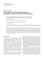
6.4. Rate Adaptation. For 64-QAM with the DaVinci codes
of length N = 480 code symbols and rates Rc ∈
{1/2, 2/3, 3/4, 5/6}, we obtain the following word error rate
(WER) curves.
For a target WER of 10−3 , this leads to the SNR thresholds
of Table 1.

Figure 9: Word error rate (WER) for nonbinary LDPC codes
at various rates. The high slopes of the curves allow to define
thresholds for the various rates, such that a very low word error rate
(<10−3 ) is achieved beyond the threshold, while it rapidly increases
before such thresholds.

6.5. Simulation Results. In the following, the channel is block
Rayleigh fading with average SNR γ. For M = 5 users, sum
rates for the proposed system and for the benchmark system
are depicted in Figure 10.
Next, we consider two users, where the first one has
average SNR γ1 and the second one γ2 = 0.1γ1 , that is, 10 dB
less. The resulting rates are depicted in Figure 11.

As before, the error rate is very low in both cases (the
adaptation is designed such that Pw < .001, and this is
fulfilled.)

7. Implementation
In this section, we discuss some issues arising by the
application of our proposed scheme. In particular we discuss
a generalization of network groups, in order to apply our
method to a real system, the effects of packet fragmentation
due to the use of different code rates and the implications our
method has on system fairness.
7.1. Generalized Network Group. In Section 2, we assumed
that, at each transmission, the source combines so that each
of the sinks knows all but one of the packets. This assumption
can be relaxed, leading to a more general case which makes
our scheme usable in most situations arising in practice.


10

EURASIP Journal on Wireless Communications and Networking

Table 1: In the table the information packet length K and the coding rate Rc are indicated for each SNR threshold. Note that for each
threshold we have: K/Rc = 480, that is, all encoded packets have the same length.
K
Rc
SNR (dB)

0
0

−∞

240
1/2
11

320
2/3
14.4

360
3/4
15.9

480
1
27

¯
¯
Block fading, 2 users, γ2 = 0.1γ1

Block fading, 5 users
6

25

5

20

4
R1 , R2

30

Sum rate

400
5/6
17.5

15

3

10

2

5

1

0

0
10

15

20
25
30
¯
Average SNR γ (dB)

35

40

Benchmark
Rate-adaptive

10

15

20
25
30
¯
Average SNR γ1 (dB)

Benchmark, user 1
Benchmark, user 2

Figure 10: Sum rate for AIR and CIR systems for a Network Coding
group with M = 5 nodes. Variable rate nonbinary LDPC codes
with 64 QAM modulation have been used. The high values of the

rates are due to NC gain. We see how AIR system gains about
2 bits/channel use in the higher SNR range. It is interesting to note
that almost the same gain has been calculated in Section 5 when
considering the average achievable rates for CIR and AIR systems
with the same number of nodes at lower SNRs.

Let us consider a generalized network group of size M. The
source has a set of packets US while sink j has a set of packets
U j lacking one or more packets in US . Let us now define the
set U∗ j as
∩\
U∗ j = U1 ∩ · · · ∩ U j −1 ∩ Ucj ∩ U j+1 ∩ · · · ∩ UM ,
∩\
(30)
where Ucj denotes the complement of U j . In other words,
U∗ j represents all packets which are common to all sinks
∩\
but sink j. The source transmits to node j one of the packets
in the set US ∩ U∗ j (i.e., all packets in U∗ j which are
∩\
∩\
known to the source node). Thus, if we indicate with |U| the
cardinality of set U, the sink j will need |US ∩ U∗ j | linearly
∩\
independent (in GF(q)) packets in order to decode all the
|US ∩ U∗ j | original native packets [19]. Such l.i. packets can
∩\
be obtained from the same source node or from other nodes
in the network which previously stored the packets. With
such scheme a total of max j (|Uc |) transmission phases are

i
needed for all the sinks to know all the packets. As a special
case, if |US ∩ U∗ j | = 1 for all j, we have the NG considered
∩\
in Section 2.

35

40

Rate-adaptive, user 1
Rate-adaptive, user 2

Figure 11: Comparison of the rates of two nodes belonging to
a Network Coding group with M = 2 nodes in both AIR and
CIR systems. One of the nodes suffers from a higher path loss
attenuation (10 dB) with respect to the other. Node with better
channel in AIR system achieves higher rate with respect to node
with better channel in CIR system. The gain arises from adapting
the coding rate of each node to the channel independently from the
other nodes.

In order to understand how to proceed when more than
one packet is unknown at one or more sinks, define an Mdimensional vector space associated to the source packet
set US . A canonical basis for this space is defined as e1 =
[10 · · · 0] · · · eM = [0 · · · 01]. The transmitted packet is a
linear combination of this basis, x = a1 ∗ e1 + · · · + aM ∗ eM .
The sets of missing packets in sink i, Uc , define a
i
|Uc |-dimensional space. In the concept of network group

i
described in Section 2, the transmitted packet is obtained as
x = e1 + · · · + eM , which is linearly independent from the
subspace spanned by the packets owned by sinks 1 · · · M. As
a result, the packets contained in each sink together with x
span the whole space IS , therefore all packets can be decoded.
In a more general case, where more than one packet
is unknown by one or more sinks, we need to transmit a
number of packets that, along with the subspaces spanned
by the packets of sinks 1 · · · M, span the whole US .
Transmitting maxi (|Uc |) linear combinations of packets is
i
sufficient to achieve this goal.


EURASIP Journal on Wireless Communications and Networking

P1

P2

P3

P6

P4

N2

P5

P6

N1
γ2

γ1

P1

S

P2

P3

P4

P5

P6

γ3

P1

N3

P3

P4

P5

Figure 12: In the setup the three sinks have three distinct subsets of
packets in S’s buffer and channels from S to each of the sinks have a
different SNR.

x(1)
x(N −2)

N

x(N −1)

R
N

.
.
.

x(N)
0

R
3

R
2

R

Figure 13: Virtual representation of event A. Random variables
x1 , . . . , xM are sorted in ascending order in sequence x(1) , . . . , x(M) .
According to the definition of event A the vth variable must assume
a value less or equal R/(M − v + 1).

In Figure 12, an example is given which clarifies the
concept just described. In the setup the three sinks have
three distinct subsets of packets and channels from S to
each of the sinks have SNRs γ1 , γ2 and γ3 . Table 2 gives a
possible scheduling and transmission solution for the setup
in Figure 12 by applying the method we just described
together with channel adaptation.
In particular, during the transmission the source broadγ
γ
γ
casts a packet obtained by adding packets p41 , p12 , and p63 ,
γ1
where p4 is packet p4 after channel encoding adapted to
γ1 . Once sink 1 receives p4 , it needs packet p5 . Next packet
γ
γ
γ
transmitted by S is p51 added with p32 and p23 for sinks 2 and
γ2
3, respectively. Finally packet p2 is transmitted to sink 2.
7.2. Packet Fragmentation and Fairness. Our proposed solution implicitly assumes that native packets can be fragmented. Each native packet u can be considered as a length
K buffer. In order to match the optimal rate on the channel,

only a part of the buffer u is sent over the channel during a
time slot on size N coded packet. In the following, we discuss
how to handle native packet fragmentation at the network
level.

11

Scheduling in Packet Fragmentation. When a node requests a
packet that needs to be fragmented the first part of the packet
is always sent out first. This avoids that different nodes in
the network have nonoverlapping parts of the same native
packet, which could make the formation of network coding
groups more difficult. Let us now consider the case in which a
given node i requests a fragment fv of a given native packet ui .
In this case, nodes belonging to its NC group do not need to
know the whole native packet. It is sufficient that the portion
they know of native packet ui include fragment fv .
Capacity and NC Group Limits. The maximum rate at which
a given node in a network group can receive data is actually
limited by two factors. One is the capacity of the physical
link between source and node (capacity-limited rate). The
other factor that limits the transmission rate is the minimum
across the nodes of the NC group of the portion of packet
ui . If such portion has length K , then the maximum
transmission rate for packet ui during a packet slot must be
less than K /N, otherwise not all nodes in the NC group
will be able to correctly decode the packet addressed to
them (NC group-limited rate). The last factor must be taken
into account in the formation of the NC group. In order to
avoid such situation we can impose that a packet cannot be

transmitted before it has been completely received.
Fairness Improvement. Shadowed users in a network would
probably experience a high packet loss rate. The CIR
approach penalizes those nodes, as their channels will have
a low capacity. By adapting the rate to each of the nodes’
channel conditions we can guarantee that users which experience shadowing for a long time (e.g., because of big urban
barriers) are not totally excluded from the communication.
This is likely to increase fairness and decrease delay in the
system.
These are some side effects at network level of our proposed method. The global behavior of a network in terms of
aggregated throughput, reliability, delay, and fairness where
such transmission scheme is used need to be quantified by
means of analytical/numerical methods, and is beyond the
scope of this paper.

8. Conclusion
In this paper we proposed a new approach for rate adaptation
in opportunistic scheduling. Such approach applies channel
adaptation techniques originally proposed for asymmetric
TWRC communication to a network context. After system
model definition at both packet level (network group) and
physical level (channel statistics), we described previously
proposed methods for transmission scheduling in NC. We
carried out a comparison between our method (adaptive
information rate) and the scheduling method typically
used in nc (constant information rate) from a information
theoretical point of view. We obtained expression for the cdf
of achievable rates for CIR system and a lower bound for
AIR system’s cdf. We also calculated an approximation to
AIR cdf at low SNRs and showed that cdf of CIR systems

12

EURASIP Journal on Wireless Communications and Networking

Table 2: Scheduling solution for the setup of Figure 12. txk indicates the transmission phase. Each phase corresponds to the complete
transmission of a native packet (or a sum of native packets).
Trx phase
U1
0
p1 , p2 , p3 , p6
1
p1 , p2 , p3 , p6 , p4
2
p1 , p2 , p3 , p4 , p5 , p6
3
p1 , p2 , p3 , p4 , p5 , p6

US ∩ U∗ 1
∩\
p4 , p5
p5

U2
p4 , p5 , p6
p4 , p5 , p6 , p1
p1 , p3 , p4 , p5 , p6
p1 , p2 , p3 , p4 , p5 , p6

is an upper bound that of AIR system. We implemented a
simulator using nonbinary LDPC codes developed in the
DaVinci project [17] and showed that our method allows
a better exploitation of good channels with respect to CIR
method. This was shown to increase throughput at each
transmission. We then discussed some issues that arise from
the modifications at physical level brought from AIR method
in a network coding scenario. Such issues will be extensively
analyzed and their impact quantified in our future works, as
well as a system-level throughput analysis gain. New coding
techniques can also be investigated in order to fully exploit
achievable throughput and fairness enhancements in AIR
systems.

Appendices
In the following, we derive the calculation for the cumulative
density function of the achievable rate for the system with
constant information rate and the approximation for the cdf
of the adaptive information rate system we proposed in this
paper. We talk about achievable rates and not capacity as we
are not optimizing with respect to power.

A. Constant Information Rate
Channel coefficients are i.i.d. exponentially distributed random variables with mean value γ. Their marginal pdf is then
1
fΓ γ = e−γ/γ u γ .
γ

(A.2)

We will use round brackets to indicate variables sorted
in ascending order, that is, γ(1) is the smallest among
variables γ(v) . As stated in Section 5, the cdf for the constant
information rate system is given by:
FRcir (R) = P {Rcir < R}
=P

max

v∈{1,...,M }

(M − v + 1)log2 1 + γ(v)

(A.3)

Let us introduce the following notation:
xv = log2 1 + γv ,
x(v) = log2 1 + γ(v) ,

U3
p1 , p3 , p4 , p5
p1 , p3 , p4 , p5 , p6
p1 , p2 , p3 , p4 , p5 , p6
p1 , p2 , p3 , p4 , p5 , p6

US ∩ U∗ 3
∩\
p6
p2

Transmitted
γ
γ
γ
p4 1 ⊕ p1 2 ⊕ p6 3
γ1
γ2
γ
p5 ⊕ p3 ⊕ p2 3
γ2
p2

and finally
z=

max

v∈{1,...,M }

(M − v + 1)log2 1 + γv

= Rcir .

(A.5)

Using (A.5) in (A.3) we can write
Fcir (R) = P {z < R} = FZ (R),

(A.6)

where FZ (R) is the cumulative distribution function of the
variable z calculated in point R. The function FZ (R) is, by
definition
FZ (R) = P Mx(1) < R, (M − 1)x(2) < R, . . . , x(M) < R .
(A.7)
Note that the smaller the variable x(v) , the higher the
multiplying coefficient M − v + 1.
We can rewrite the (A.7) as
FZ (R) = P x(1) <

R
R
, x(2) <
, . . . , x(M) < R . (A.8)
M
M−1

Let us indicate the event inside brackets as A. Figure 13 gives
a graphical representation of event A.
We can calculate the probability of event A by using the
law of total probability
M

FZ (R) =

P { A ∩ Bi } ,

(A.9)

i=1

(A.1)

Let us sort channel coefficients of the M receivers in
ascending order, namely,
γ(1) < γ(2) < · · · < γ(M −1) < γ(M) .

US ∩ U∗ 2
∩\
p1 , p3
p3
p2

where Bi are disjoint events partitioning the area of the
sample space to which A belongs. Let us choose as Bi the
event “ jn out of M variables fall in the interval [R/(n +
1), R/n]” for all n ∈ {1, 2, . . . , M } and putting R/(M + 1) = 0
and M 1 jn = M. The intersection with A imposes on Bi the
n=
further constraint
jn ≤ n,

∀n ∈ {1, 2, . . . , M }.

(A.10)

Let us give an example to clarify the definitions given
up to now for the case with M = 2 nodes. We have two
i.i.d. random variables x1 and x2 . We sort them and call

the smallest one x(1) and the biggest one x(2) . Event A is,
by definition: A = {x(1) < R/2, x(2) < R}. Events Bi , with
i ∈ {1, 2, 3} are the following:
(i) B1 = “2 variables fall in the interval [R/2, R] and 0
variables fall in the interval [0, R/2]”;

(A.4)

(ii) B2 = “2 variables fall in the interval [0, R/2] and 0
variables fall in the interval [R/2, R]”;


EURASIP Journal on Wireless Communications and Networking
(iii) B3 = “1 variable falls in the interval [R/2, R] and 1
variable falls in the interval [0, R/2]”.
It is easy to see that these are disjoint events which partition
the sample space, that is, they take into account all the
possible ways in which the two variables can be distributed
in the two intervals. In order to calculate the (A.9), we need
to find the intersection between event A and each of the Bi .
It can be easily verified that such intersection can be found
by adding to each Bi the constraint (A.10), which, for M = 2,
can be expressed as “the number of variables that fall in the
interval [R/2, R] must be less than or equal to 1 and the
number of variables that fall in the interval [0, R/2] must be
less than or equal to 2”. This implies that the (A.9) is given
by the sum of the probabilities of events B2 and B3 . Note that
events Bi do not consider sorted variables, as the sorting is
implicitly defined in the definition of such events. This allows
to consider the variables as i.i.d, which makes calculation of

events Bi easier.
A similar calculation can be done for a generic number M
of nodes. As seen in the example, the calculation reduces to
defining events Bi , choose those which describe event A and
sum their probabilities. Such probabilities can be calculated
as follows. The probability that a generic variable xv =
log2 (1 + γv ) (unsorted) falls in the interval [R/(n + 1), R/n] is
equal to FX (R/n) − FX (R/(n+1)), FX (x) being the cumulative
density function of x. FX (x) can be obtained transforming
the exponential r.v. γ
FX (x) = e1/γ e−1/γ − e−2 /γ u(x),
x

(A.11)

where u(x) is a function that assumes value 0 for x <
0, 1 for x > 0 and 1/2 in 0. Because of independency
among the variables, we can calculate the probability that
jn variables fall in the interval [R/(n + 1), R/n], which is
[FX (R/n) − FX (R/(n + 1))] jn . From now on, we will indicate
with αn the difference FX (R/n) − FX (R/n + 1). We can now
express the probability of the union of events Bi with the
formula (A.12)
M

P { Bi }

13

number n. Finally, including constraint (A.10) we obtain

expression (A.13)
FZ (R)
M

=

P { A ∩ Bi }
i=1
1 M − j1 min(2− j1 ,M − j1 − jM ) min(2− j1 − j2 ,M − j1 − j2 − jM )

=
j1 =0 jM =1

j3 =0

min(M −2− j1 −···− jM −3 ,M − j1 − j2 −···− jM −3 − jM )

···
jM −2 =0

×

M!
j j
jM − M − j − j −···− jM −2 − jM jM
αM .
α 1 α 2 · · · αM −22 αM −11 2
j1 ! · · · jM ! 1 2
(A.13)

B. Adaptive Transmission
B.1. CDF in the Low SNR Regime. Let us indicate with ci the
(unsorted) instantaneous capacity of the link between source
and receiver i. Let us recall from Section 5 that an achievable
rate for such system is
M

Radapt =

⎧
⎨M

FRair (c) = P ⎩

ci = log2 1 + γi ,

(B.15)

(B.16)

γi being an exponentially distributed random variable with
mean value E{γi } = γi = γ.
1 (which is the case most of the time in
When γi
the SNR regime), we can approximate the logarithm with its
Taylor expansion at the second term, that is

M

···

γi
.
ln(2)

(B.17)

M

ci
i=1

jM −1 =0

j1 ! · · · jM !

ci < c⎭,

where

Rair =

M − j1 − j2 −···− jM −3 − jM −2

×

⎫
⎬

Thus, we have

j3 =0

j j
α11 α22

i=1

ci = log2 1 + γi

=

(B.14)

We wish to calculate an approximation for the cdf of Cair
in the low SNR regime. By definition the cdf of Rair is

M M − j1 M − j1 − j2

M!

ci .
i=1

i=1

j1 =0 j2 =0

j2 =0

M
γi
= γi .
ln(2) i=1
i=1

(B.18)

Using expression (B.18) we can calculate the pdf of Rair as
jM −2 jM −1 jM − j − j −···− jM −2 − jM −1
· · · αM −2 αM −1 αM 1 2
,

(A.12)
where the coefficient M!/ j1 ! · · · jM ! is the number of partitions of M elements in M bins putting jn elements in bin

fRair (c) = fγ1 (c) ⊗ fγ2 (c) ⊗ · · · ⊗ fγM (c).

(B.19)

By substituting the expression of fγ1 (c) in (B.19) we find
fRair (c) =

cM −1 e−c/γ
u(c),
(M − 1)!γM

(B.20)

14

EURASIP Journal on Wireless Communications and Networking

and finally:
low
FRair (c) =

c
0

M −1
c ln(2)/γ
xM −1 e−x/γ
−c ln(2)/γ
.
M dx = 1 − e
v!
(M − 1)!γ
v=0
(B.21)
v

At higher SNR the (B.24) is a loose lower bound for the cdf
of Cair , in fact we have the following inequalities:
γi =

γi
> log2 1 + γi = ci ,
ln(2)

M

⎧
⎨M

low
FRair (c) = P ⎩

i=1

i=1

⎫
⎬

ci ,
i=1

⎧
⎨M

γi < c ⎭ < P ⎩

i=1

(B.23)

R
R
− FC

M
M+1

+ FC

R
M−1

R
M

FC

M −2

MR
MR
,
− FC
M
M+1
(B.29)

+FC

the FC (c) being the cdf of the random variable c = log2 (1+γ).
We recall the expression for the FC (c)
FC (c) = e1/γ e−1/γ − e−2 /γ u(c).
c

ci < c⎭ = FRair (c). (B.24)

R
R
, . . . , cM < R .
δ = c 1 < , . . . , ci <
M
M−i+1

(B.25)

Now it is sufficient to prove that the following two propositions are true
β ⊂ δ,

(B.26)
P {s} > 0.

(B.27)

Let us start with the (B.26). For β to be verified, at least one
of the ci must be be greater than R. Moreover, if we impose that c j < R/M
for a given j, there must be at least another ci such that
ci < (R/(M − 1)). If this is not verified there will be M − 1 ci
for which ci > (R/(M − 1)) plus c j , so the total sum would be
greater than R. Iterating this M times we will obtain exactly
the condition δ which, as just shown, must be verified for the
β to be true. Now let us consider the (B.27). We can take as
condition s the following:
s=

= FC

⎫
⎬

B.2. Upper Bound of cdf. We now show that the (16) upper
bounds the cdf of the achievable rate for the AIR system.
Let us start by modifying the condition in brackets in the
(B.15) that we will call condition β. We relax such condition
so that it be verified with higher probability for each R. Such
condition says that the sum of capacities in all links must not
exceed R. We want to find a condition δ so that if β is true
also δ is true, but there must exist a set of events with non
zero probability for which if δ is verified β is not. For this
purpose, let us put δ = A, where A is the event that defines
the cdf of cir system (see Appendix A), that is

∃s ⊂ δ | s ⊆ β,
/

P {s}

(B.22)

M

γi >

show that P {s} > 0. The probability of s is a finite quantity

given by

R R
R
R
< c1 < ,
< c2 <
,
M+1
M M
M−1
R
R
MR
...,
< cM −1 <
,
< cM < R .
M
M−1 M+1

(B.28)

It can be easily seen that s ⊂ δ. The minimum value for the
sum of all ci under condition s is R(2 − 2/M) which is greater
than R for M
2. This means that s ⊆ β. We have left to
/

(B.30)

B.3. Lower Bound. In order to find a lower bound for the cdf
of AIR system, we introduce the following constraint to the
condition inside brackets in the (B.15)
ci <

R
, ∀i ∈ {1, 2 . . . , M }.
M

(B.31)

Adding (B.31) in (B.15) we obtain the following expression:
⎫

⎧
⎨M

⎬
R
Fadapt (R) = P ⎩ ci < R, ci < , ∀i ∈ {1, 2, . . . , M }⎭
M
i=1
−

= P ci <

R
M R
, ∀i ∈ {1, 2, . . . , M } = Fci

M
M

= eM/γ e−1/γ − e−2

R/M /γ

M

.
(B.32)

Acknowledgments
The authors would like to thank Dr. Deniz Gunduz for
the helpful discussions made during the development of
present work. This work was partially supported by the
Spanish Government through Project m:VIA (TSI-0203012008-3), by the European Commission by INFSCO-ICT216203 DaVinci (Design And Versatile Implementation of
Nonbinary wireless Communications based on Innovative
LDPC Codes) and the Network of Excellence in Wireless
COMmunications NEWCOM++ (Contract ICT-216715),
and by Generalitat de Catalunya under Grant 2009-SGR940. G. Cocco is partially supported by the European Space
Agency under the Networking/Partnering Initiative.

References
[1] R. Ahlswede, N. Cai, S.-Y. R. Li, and R. W. Yeung, “Network
information flow,” IEEE Transactions on Information Theory,
vol. 46, no. 4, pp. 1204–1216, 2000.
[2] C. Fragouli and E. Soljanin, “Network coding fundamentals,”
Foundations and Trends in Networking, vol. 2, no. 1, pp. 1–133,
2007.

[3] D. S. Lun, M. M´ dard, R. Koetter, and M. Effros, “On coding
e
for reliable communication over packet networks,” Physical
Communication, vol. 1, no. 1, pp. 3–20, 2008.


EURASIP Journal on Wireless Communications and Networking
[4] C. E. Shannon, “A mathematical theory of communication,”
The Bell System Technical Journal, vol. 27, pp. 379–423, 623–
656, 1948.
[5] L. R. Ford Jr. and D. R. Fulkerson, “Flows in networks,” Tech.
Rep., United States Air Force Project RAND, August 1962.
[6] T. Ho, R. Koetter, M. M´ dard, D. R. Karger, and M. Effros,
e
“The benefits of coding over routing in a randomized
setting,” in Proceedings of the IEEE International Symposium
on Information Theory (ISIT ’03), p. 442, June-July 2003.
[7] T. Ho, M. M´ dard, R. Koetter et al., “A random linear
e
network coding approach to multicast,” IEEE Transactions on
Information Theory, vol. 52, no. 10, pp. 4413–4430, 2006.
[8] J.-S. Park, M. Gerla, D. S. Lun, Y. Yi, and M. M´ dard, “Codee
Cast: a network-coding-based ad hoc multicast protocol,”
IEEE Wireless Communications, vol. 13, no. 5, pp. 76–81, 2006.
[9] S. Katti, H. Rahul, W. Hu, D. Katabi, M. Medard, and
J. Crowcroft, “XORs in the air: practical wireless network
coding,” IEEE/ACM Transactions on Networking, vol. 16, no.
3, pp. 497–510, 2008.
[10] H. Yomo and P. Popovski, “Opportunistic scheduling for
wireless network coding,” IEEE Transactions on Wireless Communications, vol. 8, no. 6, pp. 2766–2770, 2009.

[11] S.-L. Gong, B.-G. Kim, and J.-W. Lee, “Opportunistic scheduling and adaptive modulation in wireless networks with
network coding,” in Proceedings of the 69th IEEE Vehicular
Technology Conference (VTC ’09), pp. 1–5, April 2009.
[12] M. Effros, M. Medard, T. Ho, S. Ray, D. Karger, and R.
Koetter, “Linear network codes: a unified framework for
source, channel, and network coding,” in Proceedings of the
DIMACS Workshop on Network Information Theory, 2003.
[13] C. Hausl, “Improved rate-compatible joint network-channel
code for the two-way relay channel,” in Proceedings of the
Joint Conference on Communications and Coding (JCCC 06),
Să lden, Austria, March 2006.
o
[14] J. Hou, C. Hausl, and R. Kă tter, Distributed turbo coding
o
schemes for asymmetric two-way relay communication,” in
Proceedings of the 5th International Symposium on Turbo Codes
and Related Topics, pp. 237–242, September 2008.
[15] E. Tuncel, “Slepian-Wolf coding over broadcast channels,”
IEEE Transactions on Information Theory, vol. 52, no. 4, pp.
1469–1482, 2006.
[16] T. M. Cover and J. A. Thomas, Elements of Information Theory,
Wiley-Interscience, New York, NY, USA, 1991.
[17] />[18] S. Pfletschinger, A. Mourad, E. L´
opez, D. Declercq, and G.
Bacci, “Performance evaluation of non-binary LDPC codes,”
in Proceedings of the ICT Mobile Summit, Santander, Spain,
June 2009.
[19] P. A. Chou, Y. Wu, and K. Jain, “Practical network coding,” in
Proceedings of the 51st Allerton Conference on Communication,
Control and Computing, October 2003.

15