Báo cáo hóa học: " Research Article Crystallized Rate Regions for MIMO Transmission" doc

Hindawi Publishing Corporation
EURASIP Journal on Wireless Communications and Networking
Volume 2010, Article ID 919072, 17 pages
doi:10.1155/2010/919072
Research Article
Crystallized Rate Regions for MIMO Transmission
Adrian Kliks (EURASIP Member),
1
Pawel Sroka (EURASIP Member),
1
and Merouane Debbah
2
1
Poznan Univer sity of Technology, Chair of Wireless Communications, Polanka 3, 60-965 Poznan, Poland
2
SUPELEC, Alcatel-Lucent Chair on Flexible Radio, 3 rue Joliot-Curie, 91192 Gif-sur-Yvette, France
Correspondence should be addressed to Pawel Sroka,
Received 1 February 2010; Revised 2 July 2010; Accepted 8 July 2010
Academic Editor: Osvaldo Simeone
Copyright © 2010 Adrian Kliks et al. This is an open access article distributed under the Creative Commons Attribution License,
which permits unrestricted use, distribution, and reproduction in any medium, provided the original work is properly cited.
When considering the multiuser SISO interference channel, the allowable rate region is not convex and the maximization of the
aggregated rate of all the users by the means of transmission power control becomes inefficient. Hence, a concept of the crystallized
rate regions has been proposed, where the time-sharing approach is considered to maximize the sumrate.In this paper, we extend
the concept of crystallized rate regions from the simple SISO interference channel case to the MIMO/OFDM interference channel.
As a first step, we extend the time-sharing convex hull from the SISO to the MIMO channel case. We provide a non-cooperative
game-theoretical approach to study the achievable rate regions, and consider the Vickrey-Clarke-Groves (VCG) mechanism design
with a novel cost function. Within this analysis, we also investigate the case of OFDM channels, which can be treated as the special
case of MIMO channels when the channel transfer matrices are diagonal. In the second step, we adopt the concept of correlated
equilibrium into the case of two-user MIMO/OFDM, and we introduce a regret-matching learning algorithm for the system to
converge to the equilibrium state. Moreover, we formulate the linear programming problem to find the aggregated rate of all users

and solve it using the Simplex method. Finally, numerical results are provided to confirm our theoretical claims and show the
improvement provided by this approach.
1. Introduction
The future wireless systems are characterized by decreasing
range of the transmitters as higher transmit frequencies are
to be utilized. The decreasing cell sizes combined with the
increasing number of users within a cell greatly increases the
impact of interference on the overall system performance.
Hence, mitigation of the interference between transmit-
receive pairs is of great importance in order to improve the
achievable data rates.
The Multiple Input Multiple Output (MIMO) technol-
ogy has become an enabler for further increase in system
throughput. Moreover, the utilization of spatial diversity
thanks to MIMO technology opens new possibilities of
interference mitigation [1–3].
Several concepts of interference mitigation have been
proposed, such as the successive interference cancellation
or the treatment of interference as additive noise, which
are applicable to different scenarios [4–6]. When treating
the interference as noise the, n-user achievable rates region
has been found to be the convex hull of n hypersurfaces
[7]. A novel strategy to represent this rate region in the n-
dimensional space, by having only on/off power control has
been proposed in [8]. A crystallized rate region is obtained by
forming a convex hull by time-sharing between 2
n
−1corner
points within the rate region [8].
Game-theoretic techniques based on the utility maxi-

mization problem have received significant interest [7–10].
The game-theoretical solutions attempt to find equilibria,
where each player of the game adopts a strategy that they
are unlikely to change. The best known and commonly used
equilibrium is the Nash equilibrium [11]. However, the Nash
equilibrium investigates only the individual payoff, and that
may not be efficient from the system point of view. Better
performance can be achieved using the correlated equilib-
rium [12], in which each user considers the others’ behaviors
to explore mutual benefits. In order to find the correlated
equilibrium, one can formulate the linear programming
2 EURASIP Journal on Wireless Communications and Networking
problem and solve it using one of the known techniques,
such as the Simplex algorithm [13]. However, in case of
MIMO systems, the number of available game strategies is
high, and the linear programming solution becomes very
complex. Thus, a distributed solution can be applied, such
as the regret-matching learning algorithm proposed in [8],
to achieve the correlated equilibrium at lower computational
cost. Moreover, the overall system performance may be
further improved by an efficient mechanism design, which
defines the game rules [14].
In this paper, the rate region for the MIMO interference
channel is examined based on the approach presented in
[8, 15]. Specific MIMO techniques have been taken into
account such as transmit selection diversity, spatial water-
filling, SVD-MIMO, or codebook-based beamforming [16–
19]. Moreover, an application of the correlated equilibrium
concept to the rate region problem in the considered
scenario is presented. Furthermore, a new Vickey-Clarke-

Groves (VCG) auction utility [11] formulation and the
modified regret-matching learning algorithm are proposed
to demonstrate the application of the considered concept for
the 2-user MIMO channel.
The reminder of this paper is structured as follows.
Section 2 presents the concept of crystallized rates region
for MIMO transmission. Section 3 describes the applica-
tion of correlated equilibrium concept in the rate region
formulation and presents the linear programming solution
for the sum-rate maximization problem. Section 4 outlines
the mechanism design for application of the proposed
concept in 2-user interference MIMO channel, comprising
the VCG auction utility formulation and the modified
regret-matching learning algorithm. Moreover, specific cases
of different MIMO precoding techniques, including the
ones considered for future 4G systems such as the Long
Term Evolution-Advanced (LTE-A) [20, 21], and Orthogonal
Frequency Division Multiplexing (OFDM) transmission are
presented as examples of application of the derived model.
Finally, Section 5 summarizes the simulation results obtained
for the considered specific cases, and Section 6 draws the
conclusions.
2. Crystallized Rate Regions for
MIMO/OFDM Transmission
In this section, we present the generalization of the concept of
crystallized rate regions in the context of the OFDM/MIMO
transmissions. We start with defining the channel model
under study and follow by the analysis of the achievable
rate regions for the interference MIMO channel, when
interference is treated as Gaussian noise. Finally, the gener-

alized definition of the rate regions for the MIMO/OFDM
transmission will be presented.
2.1. System Model for 2-User Interference MIMO Channel.
The multicell uplink interference MIMO channel is con-
sidered in this paper. Without loss of generality and for
the sake of clarity, the channel model consists in the 2-
user 2-cell scenario, in which each user (denoted as the
Mobile Terminal (MT)) communicates with his own Base
Station (BS) causing interference to the neighboring cell
(see Figure 1(a)). Each MT is equipped with N
t
(transmit)
antennas, and each BS has N
r
(receive) antennas. Moreover,
user i can transmit data with maximum total power P
i,max
.
Perfect channel knowledge in all MTs is assumed. In order to
ease the analysis, we limit our derivation to the 2
×2MIMO
case (see Figure 1(b)), where both the transmitter and the
receiver use only two antennas.
User i transmits the signal vector X
i
∈ C
2
through the
multipath channel H
∈ C

4×4
,where
H
=

H
11
H
12
H
21
H
22

, H
i, j
∈ C
2×2
. (1)
The channel matrix H
i, j
={h
(i, j)
k, l
∈ C,1≤ k, l ≤ 2} consists
of the actual values of channel coefficients h
(i, j)
k, l
, which define
the channel between transmit antenna k at the ith MT and

the receive antenna l at the jth BS. In the considered 2-user
2
× 2 MIMO case, only four channel matrices are defined,
that is, H
11
, H
22
(which describe channel between the first
MT and first BS or second MT and second BS, resp.), H
12
,
and H
21
(which describe the interference channel between
first MT and second BS and between second MT and first
BS, resp.). Additive White Gaussian Noise (AWGN) of zero
mean and variance σ
2
is added to the received signal. Receiver
i observes the useful signal, denoted as Y
i
, coming from the
ith user. Moreover, in the interference scenario, receiver i
(BS
i
) receives also interfering signals from other users located
at the neighboring cell Y
j
, j
/

=i. Interested readers can find
solid contribution on the interference channel capacity in the
rich literature, for example, [1, 2, 22, 23]. When interference
is treated as noise, the achievable rates for 2-user interference
MIMO channel are defined as follows [22]:
R
1
(
Q
1
, Q
2
)
= log
2

det

I + H
11
Q
1
H
∗
11
·

σ
2
I + H

21
Q
2
H
∗
21

−1

,
R
2
(
Q
1
, Q
2
)
= log
2

det

I + H
22
Q
2
H
∗
22

·

σ
2
I + H
12
Q
1
H
∗
12

−1

,
(2)
where R
1
and R
2
denote the rate of the first and second user,
respectively, (A
∗
) denotes transpose conjugate of matrix A,
det(A) is the determinant of matrix A,andQ
i
is the ith user
data covariance matrix, that is, E
{X
i

X
∗
i
}=Q
i
and tr(Q
1
) ≤
P
1, max
,tr(Q
2
) ≤ P
2, max
. We define the rate region as R =

{
(R
1
(Q
1
, Q
2
), R
2
(Q
1
, Q
2
))}.

One can state that the formulas presented above allow
us to calculate the rates that can be achieved by the users in
the MIMO interference channel scenario in a particular case
when no specific MIMO transmission technique is applied.
Such approach can be interpreted as a so-called Transmit
Selection Diversity (TSD) MIMO technique [16], where the
BS can decide between one of the following strategies: to put
all of the transmit power to one antenna (N
t
strategies, where
N
t
is the number of antennas), to be silent (one strategy), or
to equalize the power among all antennas (one strategy).
EURASIP Journal on Wireless Communications and Networking 3
N
r
H
11
N
t
H
12
H
21
1
2
N
t
H

22
N
r
(a)
X
1
X
2
MT 1
MT 2
h
(11)
11
h
(11)
12
h
(12)
11
h
(12)
12
h
(11)
21
h
(11)
22
h
(12)

21
h
(12)
22
h
(21)
11
h
(21)
12
h
(22)
11
h
(22)
12
h
(21)
21
h
(21)
22
h
(22)
21
h
(22)
22
Y
1

Y
2
BS 2
BS 1
(b)
Figure 1: MIMO interference channel: general 2-cell 2-user model (a) and the details representation of the considered 2 × 2case(b).
When the channel is known at the transmitter, the
channel capacity can be optimized by means of some well-
known MIMO transmission techniques. Precisely, one can
decide for example to linearize (diagonalize) the channel by
the means of Eigenvalue Decomposition (EvD) or Singular
Value Decomposition (SVD) [16, 17, 24]. Such approach will
be denoted hereafter as SVD-MIMO.v Moreover, in order to
avoid or minimize the interference between the neighboring
users within one cell, BS can precode the transmit signal.
In such a case, the sets of properly designed transmit and
receive beamformers are used at the transmitter and receiver
side, respectively. The precoders can be either calculated
continuously based on the actual channel state information
from all users or can be defined in advance (predefined) and
stored in a form of a codebook, from which the optimal
set of beamformers is selected for each user based on its
channel condition. The later approach is proposed in the
Long Term Evolution (LTE) standard where for the 2
× 2
MIMO case a specific codebook is proposed [20]. Similar
assumption is made for the so called Per-User Unitary
Rate Control (PU
2
RC) MIMO systems, where the set of

N beamformers is calculated [18, 21]. Since the process
of finding the set of transmit and receive beamformers is
usually time and energy consuming and require accurate
Channel State Information (CSI), the optimal approaches
(where the precoders are calculated based on the actual
channel state) are replaced by the above-mentioned list of
predefined beamformers stored in a form of a codebook.
Since the number of precoders is limited, the performance
of such approach could be worse than the optimal one,
particularly in the interference channel scenario. Based on
this observation, new techniques of generation of the set of
N beamformers have been proposed. One of them is called
random-beamforming [19, 25], since the set of precoders
is obtained in a random manner. At every specified time
instant, a new set of beamformers is randomly generated,
from which the subset of precoders that optimize some
predefined criteria is selected. Simulation results given in
[19, 25]andSection 5.1 show that assuming such approach,
one can achieve the global extremum in particular when the
codebook size is large. When the set of randomly generated
beamformers is used, the set of receive beamformers has to
be calculated at the receiver. Various criteria can be used,
just to mention the most popular and academic ones: Zero-
Forcing (ZF), MinimumMean Squared Error (MMSE), or
Maximum-Likelihood (ML) [16, 17]. In our simulation, we
consider the combination of these methods, that is, ZF-
MIMO, MMSE-MIMO, and ML-MIMO, with three different
codebook generation methods—one of the size N, that is,
generated randomly (denoted hereafter as RAN-N), one
defined as proposed for LTE and one specified for PU

2
RC-
MIMO. In other words, the abbreviation ZF-MIMO-LTE
describes the situation when the transmitter uses the LTE
codebook and the set of receive beamformers is calculated
using the ZF criterion.
However, let us stress that (2) has to be modified when
one of the precoding techniques (including SVD method,
which is a particular case of precoding) is applied. Thus, the
general equations for the achievable rate computation are
defined as follows:
R
1
(
Q
1
, Q
2
)
= log
2

det

I + u
∗
1
H
11
v

1
Q
1
v
∗
1
H
∗
11
u
1
·

σ
2
u
∗
1
u
1
+ u
∗
1
H
21
u
2
Q
2
u

2
H
∗
21
u
1

−1

,
R
2
(
Q
1
, Q
2
)
= log
2

det

I + u
∗
2
H
22
v
2

Q
2
v
∗
2
H
∗
22
u
2
·

σ
2
u
∗
2
u
2
+ u
∗
2
H
12
u
1
Q
1
u
1

H
∗
12
u
2

−1

,
(3)
where u
i
and v
i
denote the set of receive and transmit
beamformers, respectively, obtained for the ith user. In a case
of SVD-MIMO, the above-mentioned vectors are obtained
by the means of singular value decomposition of the channel
transfer matrix whereas for the other precoded MIMO
systems, the set of receive coefficients is calculated as follows
[23]:
(i) for zero-forcing receiver
v
i
=


H
∗
ii

H
ii

−1
·H
∗
ii

∗
,
(4)
4 EURASIP Journal on Wireless Communications and Networking
(ii) for MMSE receiver
v
i
=
⎛
⎜
⎜
⎝
⎛
⎜
⎜
⎝
H
∗
ii
H
ii
+


j
j
/
=i
P
j
P
i
H
∗
ji
H
ji
+ σ
2
I
⎞
⎟
⎟
⎠
−1
·H
∗
ii
⎞
⎟
⎟
⎠
∗

,
(5)
(iii) for the ML receiver the elements of receive beam-
formersareequalto1(inotherwords,noreceive
beamforming is used).
The last Hermitian conjugate in (4) and in (5) is due to the
assumed definition of the achievable user rates in (3).
For comparison purposes, the spatial waterfilling tech-
nique will be considered [26], where the transmit power is
distributed among the antennas based on the waterfilling
algorithm. The spatial waterfilling approach will be denoted
hereafter as SWF-MIMO.
2.2. Achievable Rate Regions in a Case of TSD-MIMO
Interference Channel. In [8], the achievable rate regions in
the 2-user SISO scenario have been studied, where the
authors have treated the interference as Gaussian noise. It
has been stated that the rate region for the general n-user
channel is found to be the convex hull of the union of n
hyper-surfaces [7], which means that the rate regions entirely
encloses a straight line that connects any two points which
lie within the rate region bounds. In the 2-user case, the
rate regions can be easily represented as the surface limited
by the horizontal and vertical axes and the boundaries of
the 2-dimensional hypersurface (straight lines). Let us stress
that the same conclusions can be drawn for the MIMO case.
We will then discuss various achievable rate regions for the
interference MIMO channel. We will analyze the properties
of the rate regions introduced below in three cases: when the
results are averaged over 2000 channel realizations (Case A)
and for specific channel realizations (Cases B and C).

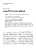
2.2.1. Rate Region for TSD-MIMO Interference Channel Case
A. The rate region for the general interference TSD-MIMO
channel is depicted in Figure 2. The results have been
obtained based on the assumption that both users transmit
with the same uniform power P
i,max
= 1 and the results have
been averaged over 2000 channel realizations, for h
(i, j)
k, l
∼
CN (0, 1, 0). One can define three characteristic points on
the border of the rate region, that is, points A, B, and
C. Specifically, point A describes the situation, where the
first user transmits with the maximum power, and Q
1
is
chosen such that Q
1
= arg max

Q
1
R
1
(

Q
1
, Q

2
= 0). Point
C can be defined in the same way as point A, but with
reference to the second user. Point B corresponds to the
situation, where both users transmit with the maximum
power and the distribution of the power among the antennas
is optimal in the sum-rate sense, that is, (Q
1
, Q
2
) =
arg max

Q
1
,

Q
2
(R
1
(

Q
1
,

Q
2
)+R

2
(

Q
1
,

Q
2
)). The first frontier
line Φ
AB
= Φ(Q
1, p
,:),p = P
1, max
,(whereQ
i, p
denotes
the covariance for which tr(Q
i
) = p) is obtained when
holding the total transmit power for the first user fixed and
0
1
2
3
4
5
6

7
8
9
012 3456789
Point A
Point B
Point C
Φ
AB
= Φ(P
1,max
,:)
Φ
BC
= Φ(:, P
2,max
)
Time-sharing line
R
1
R
2
Figure 2: Achievable rate region for the MIMO interference
channel—averaged over 2000 channel realizations.
varying the total transmit power for the second user from
zero to P
2, max
. Similarly, the second frontier line Φ
BC
=

Φ(:, Q
2, p
), p = P
2, max
, is characterized by holding the
total transmit power of the second user fixed to P
2, max
and
decreasing the total transmit power by the first user from
P
1, max
to zero. One can observe that the achievable rate
region for the two user 2
×2MIMOcaseisnotconvex,thus
the time-sharing (see Section 2.5) approach seems to be the
right way for system capacity improvement. The potential
time-sharing lines are also presented in Figure 2.
2.2.2. Rate Region for TSD-MIMO Interference Channel Case
B. Quite different conclusions can be drawn for a specific
channel realization (i.e., the obtained rate regions are not
averaged over many channel realizations), where the second
user receives strong interference (see Figure 3). In such a case,
new characteristic points can be indicated on the frontier
lines of the achieved rate region. While the points A and
C can be defined in the same way as in the previous case
(i.e., when the results were averaged), two new points D
and E appeared. All of the characteristic points define a
combination of four possible situations. These are: (a) user i
balances all the power on the first antenna (b) user i balances
all the power on the second antenna (c) user i divides the

transmit power in an optimal way among both antennas (d)
user i does not transmit. When both users chose one of the
four predefined strategies, one of the characteristic points (in
our case points A, C, D, and E) on the frontier line of the
rate regions can be reached. In Figure 3 the potential time-
sharing lines are also plotted.
2.2.3. Rate Region for TSD-MIMO Interference Channel Case
C. In Figure 4, the results obtained for another fixed channel
realization are presented mainly a case is considered, where
the first user transmits data with twice the maximum power
(i.e., P
1, max
= 2 · P
2, max
) of user 2. One can observe that
user 1 achieves significantly higher rates compared to user 2.
For this situation, similar conclusions can be drawn as for
EURASIP Journal on Wireless Communications and Networking 5
0
1
2
3
4
5
6
7
8
9
0123456
Point A

Point D
Point E
Point C
R
1
R
2
Figure 3: Achievable rate region for the MIMO interference
channel—one particular channel realization (user two observes
strong interference).
0
2
4
6
8
10
12
14
012345 67
Point A
Point D
Point E
Point C
R
1
R
2
A
∗
1

A
∗
2
A
∗
3
Figure 4: Achievable rate region for the MIMO interference
channel—the transmit power of the first user is twice higher than
the transmit power of the second user.
the situation depicted in Figure 3, that is, new characteristic
points have occurred.
Let us put the attention on the additional dashed curves
which are enclosed inside the rate region and usually start
and finish in one of the characteristic points (depicted
as small black-filled circles). These curves show the rate
evolution achieved by both users when the users decide to
choose one of the four predefined strategies. Let us define
them explicitly: user i does not transmit any data (strategy
α
(0)
i
), puts all the transmit power to the antenna number
1(strategyα
(1)
i
)or2(strategyα
(2)
i
), or distribute the total
power equally between both antennas (strategy α

(3)
i
). For
example, the line with the plus marks denotes the following
user behavior: starting from point A
∗
1
, when the first user
transmits all the power on the first antenna and the second
5
10
15
20
25
510152025
R
1
R
2
Time sharing line
SVD frontier line
SWF line / Q
(3)
−Q
(3)
line
Figure 5: Achievable rate region for the precoded MIMO interfer-
ence channel.
user is silent, the second user increases the transmit power
on the second antenna from zero to P

2, max
achieving point
A
∗
2
; user 2 transmits with fixed power on the second antenna,
and the first user reduces the power from the P
1, max
to zero
reaching point A
∗
3
. In other words, this line corresponds to
the situation when user 1 chooses strategy α
(1)
, and the user
2 selects strategy α
(2)
. The other lines below the frontiers
show what rate will be achieved by both users when they
decide to play one of the predefined strategies all the time.
Let us notice that choosing the strategy α
(0)
by one of the
user results in moving over the vertical or horizontal border
of the achievable rate region. However, such a case will not
be discussed in this paper. It is worth mentioning that the
frontier lines define the boundaries of the rate region that
corresponds to choosing the best strategy in every particular
situation by both users. In other words, the frontier line

is more or less similar to the rate achieved by both users
when every time both of them select the best strategy for the
actual value of transmit power, what can be approximated as
switching between the dashed lines in order to maximize the
instantaneous throughput?
2.3. Achievable Rate Regions for the Precoded MIMO Systems.
Similar analysis can be applied for the SVD-MIMO case.
In such a situation, the BS can also select one of the four
strategies defined in the previous subsection however, the
precoder is computed in an (sub) optimal way by the means
of SVD based on the information on the channel transfer
function. The channel transfer functions H
ij
that define the
channel between user in the ith cell and the jth BS in a
jth cell are assumed to be unknown by the neighboring
BSs. An exemplary plot of the achievable rate region for
2000 channel realizations is presented in Figure 5.Onecan
observe that the obtained rate region is concave, thus the
time-sharing approach seems to provide better results. As
in a TSD-MIMO case, the obtained results are characterized
by a higher number of corner points (degrees of freedom)
when compared to the Single-Input/Single-Output (SISO)
6 EURASIP Journal on Wireless Communications and Networking
transmission. The transmitter can select one of the corner
points in order to optimize some predefined criteria (like
minimization of interference between users). The spatial
waterfilling line is also shown in this figure which matches
the Q
(3)

−Q
(3)
line (i.e., the line when both users choose the
third strategy with equally distributed power among transmit
antennas every time and control the transmit power to
maximize the capacity). Let us stress the difference between
the SWF-line and the SVD frontier line. The former is
obtained as follows: user 1 transmit with the maximum
allowed power P
max
using SWF technique and at the same
time user 2 increases its power from 0 to P
max
.Next,
the situation is reversed—the second user transmits with
maximum allowed power and user 1 reduces the transmit
power from P
max
to 0. In other words, the covariance matrix
Q
x
is simply the identity matrix multiplied by the actual
transmit power. Contrary to this case, the SVD frontier line
represents the maximum possible rates that can be achieved
by both users for every possible realization of the covariance
matrix Q
x
, whose trace is less or equal to the maximum
transmit power, and when precoding based on SVD of the
channel transfer function has been applied. The frontier line

defines the maximum theoretic rates that can be achieved by
both users. One can observe that although both lines start
and end at the same points of the achievable rate region, the
influence of interference is significantly higher in the SWF
approach.
2.4. Achievable Rate Regions for the OFDM Systems. The
methodology proposed in the previous sections can be also
applied in a case of OFDM transmission. In such a case,
the interferences will be observed only in a situation, when
the neighboring users transmit data on the same subcarrier.
Two achievable rate regions for OFDM transmission are
presented below that is, in Figure 6, the rate region averaged
over 2000 different channel realizations is shown, and in
Figure 7, the rate region achieved for one arbitrarily selected
channel realization are presented (in particular, the channel
between the first user and its BS was worse than the second
user-channel attenuation was higher, and the maximum
transmit power of the second user was twice higher than
for the first one). In both figures, the time-sharing lines
are plotted. Moreover, the curves that show the rate region
boundaries when the users play one specific strategy all
the time are shown (represented as the dashed lines in the
figure).
The obtained results are similar to those achieved for the
MIMO case. However, some significant differences can be
found, like the difference in the achievable rates in general—
the maximum achievable rates are lower in a OFDM case
comparing to the MIMO scenario.
2.5. Crystallized Rate Regions and Time-Sharing Coefficients
for the MIMO Transmission. The idea of the crystallized rate

regions has been introduced in [8] and can be understood
as an approximation of the achievable rate regions by the
convex time-sharing hull, where the potential curves between
characteristic points (e.g., A, B, and C in Figure 2)are
replaced by the straight lines connecting these points.
0
1
2
3
4
5
6
7
8
012345678
Strategy specific
rate region
frontier curve
Time-sharing line
Rate region frontier curve
R
1
R
2
Figure 6: Achievable rate region for the OFDM interference
channel—results averaged over 2000 channel realizations.
0
1
2
3

4
5
6
7
012345678910
Strategy specific
rate region
frontier curve
Time-sharing line
Rate region
frontier curve
R
1
R
2
Figure 7: Achievable rate region for the OFDM interference
channel—one particular channel realization, maximum transmit
power of the first user is two times higher than the maximum
transmit power of the second user.
One can observe from the results shown in Figure 4
that for the MIMO case, the crystallized rate region for the
2-user scenario has much more characteristic points (i.e.,
the points where both users transmit with the maximum
power for selected strategy) than in the SISO case (see [8]
for comparison). In order to create the convex hull, only
such points can be selected, which lie on the frontier line.
Moreover, the selection of all characteristic points that lie
on border line could be nonoptimal, thus only a subset of
these points should be chosen for the time-sharing approach
(compare Figures 3 and 4).

Let us denote each point in the rate region as Φ(Q
1, p
1
,
Q
2, p
2
), that is, tr(Q
1, p
1
) = p
1
,0 ≤ p
1
≤ P
1, max
and
tr(Q
2, p
2
) = p
2
,0≤ p
2
≤ P
2, max
. Point A in Figure 2 can be
defined as Φ(P
1, max
, 0); that is, user one transmits with the

maximum total power and the second user is silent; point
C, as Φ(0, P
2, max
); that is, the first user does not transmit
EURASIP Journal on Wireless Communications and Networking 7
any data and the second user transmits with the maximum
total power; point B is defined as Φ(P
1, max
, P
2, max
); that is,
both users transmit with the maximum total power. One can
observe that these points are corner (characteristic) points of
the achievable rate region. In the 2-user 2
× 2 TSD-MIMO
channel, there exist 15 points, which refer to any particular
combination of the possible strategies. In general, for the n-
user N
t
× N
r
MIMO case, there exist (N
t
+2)
n
− 1 points;
that is, the ith user can put all power to one antenna (N
t
pos-
sibilities), divide the power equally among the antennas (one

possibility), or be silent (one possibility). We do not take into
account the case when all users are silent. In a SISO case,
N
t
= 1 and the number of strategies is limited to two (i.e.,
the division of the power equally among all antennas denotes
that all the power is transmitted through the antenna).
Following the approach proposed in [8], we state that
instead of power control problem in finding the metrics P
i
,
the problem becomes finding the appropriate time-sharing
coefficients of the (N
t
+2)
n
−1 corner points. For the 2-user
2
× 2 TSD-MIMO case, we will obtain 15 points, that is,
Θ
= [θ
k, l
]for0≤ k, l ≤ 3, which fulfill

k, l
θ
k, l
= 1. In
our case, the time-sharing coefficients relate to the specific
corner points; that is, the coefficient θ

k, l
defines the point,
where user 1 choose the strategy α
(k)
1
and user 2 selects the
strategy α
(l)
2
. Consequently, (2)canberewrittenasin(6),
where Q
(k)
i
denotes the ith user covariance matrix while
choosing the strategy α
(k)
i
. Let us stress that any solution
point on the crystallized rate border line (frontier) will
lie somewhere on the straight lines connecting any of the
neighboring characteristic points.
R
1
(
Θ
)
=

k, l
θ

k, l
·log
2

det

I + H
11
Q
(k)
1
H
∗
11
·

σ
2
I + H
21
Q
(l)
2
H
∗
21

−1

,

R
2
(
Θ
)
=

k, l
θ
k, l
·log
2

det

I + H
22
Q
(l)
2
H
∗
22
·

σ
2
I + H
12
Q

(k)
1
H
∗
12

−1

.
(6)
Similar conclusions can be drawn for the precoded MIMO
systems, where (6), that defines the achievable rate in a
time-sharing approach, has to be rewritten in order to
include the transmit and receive beamformers set (see (7))
R
1
(
Θ
)
=

k, l
θ
k, l
·log
2

det

I + u

∗
1
H
11
v
1
Q
(k)
1
v
∗
1
H
∗
11
u
1
·

σ
2
u
∗
1
u
1
+ u
∗
1
H

21
v
2
Q
(l)
2
v
∗
2
H
∗
21
u
1

−1

R
2
(
Θ
)
=

k, l
θ
k, l
·log
2


det

I + u
∗
2
H
22
v
2
Q
(l)
2
v
∗
2
H
∗
22
u
2
·

σ
2
u
∗
2
u
2
+ u

∗
2
H
12
v
1
Q
(k)
1
v
∗
1
H
∗
12
u
2

−1

.
(7)
3. Correlated Equilibrium for Crystallized
Interference MIMO Channel
In general, each user plays one of N
s
= N
c
+2strategies
α

(k)
,1 ≤ k ≤ N
c
,whereN
c
is the number of antennas in
case of TSD-MIMO and SVD-MIMO (N
c
= N
t
) whereas for
ZF/MMSE/ML-MIMO N
c
denotes the codebook size (N
c
=
N). As a result of playing one of the strategies, the ith user will
receive payoff, denoted hereafter U
i
(α
(k)
i
). The aim of each
user is to maximize its payoff with or without cooperation
with the other users. Such a game leads to the well-known
Nash equilibrium strategy α
∗
i
[27], such that
U

i

α
∗
i
, α
−i

≥
U
i
(
α
i
, α
−i
)
,
∀i ∈ S,
(8)
where α
i
represents the possible strategy of the ith user
whereas α
−i
defines the set of strategies chosen by the other
users, that is, α
−i
={α
j

}, j
/
=i,andS is the users set of the
cardinality n. The idea behind the Nash equilibrium is to find
the point of the achievable rate region (which is related to
the selection of one of the available strategies), from which
any user cannot increase its utility (increase the total payoff)
without reducing other users’ payoffs.
Moreover, in this context, the correlated equilibrium
used in [8] instead of the Nash equilibrium is defined as α
∗
i
such that

α
−i
∈Ω
−i
p

α
∗
i
, α
−i

U
i

α

∗
i
, α
−i

−U
i
(
α
i
, α
−i
)

≥
0, ∀α
i
, α
∗
i
∈ Ω
i
, ∀i ∈ S,
(9)
where p(α
∗
i
, α
−i
) is the probability of playing strategy α

∗
i
in a case when other users select their own strategies α
j
,
j
/
=i. Ω
i
and Ω
−i
denote the strategy space of user i and
all the users other than i,respectively.Theprobability
distribution p is a joint point mass function of the different
combinations of users strategies. As in [8], the inequality
in correlated equilibrium definition means that when the
recommendation to user i is to choose action α
∗
i
, then
choosing any other action instead of α
∗
i
cannot result in
higher expected payoff for this user. Note that the cardinality
of the Ω
−i
is (N
c
+2)

(n−1)
.
Let us stress out that the time-sharing coefficients θ
k, l
are the (N
c
+2)
(n−1)
point masses that we want to compute.
In such a case, the one-to-one mapping function between
any time-sharing coefficient θ
k, l
and the corresponding point
mass function p(α
(k)
i
, α
(l)
j
)ofthepointΦ(α
(k)
i
, α
(l)
j
)canbe
defined as follows:
θ
k, l
= p


α
(k)
i
, α
(l)
j

, (10)
where p(α
(k)
i
, α
(l)
j
) is the probability of user i playing the kth
strategy and user j playing the lth strategy.
8 EURASIP Journal on Wireless Communications and Networking
3.1. The Linear Programming (LP) Solution. Let us formulate
the LP problem of finding the optimal time-sharing coeffi-
cients θ
k, l
. Following [28, 29] and for the sake of simplicity,
we limit the problem to the sum-rate maximization (the
weighted sum) as presented below:
arg max
p

i∈S
E

p
(
U
i
)
s.t.

α
−i
∈Ω
−i
p

α
∗
i
, α
−i


U
(i)
α
∗
i
, α
−i
−U
(i)
α

i
, α
−i

 0,
∀α
i
, α
∗
i
∈ Ω
i
, ∀i ∈ S

α
∗
i
∈Ω
i
,
α
−i
∈Ω
−i
p

α
∗
i
, α

−i

=
1∀i 0 ≤ p

α
∗
i
, α
−i

≤
1,
(11)
where E
p
(·) denotes the expectation over the set of all
probabilities. We can limit ourselves into 2-users 2-BSs
scenario with N strategies. In such a case, the LP problem
can be presented as follows:
max
p
i, j
N

k=1
N

l=1


U
(1)
k, l
+ U
(2)
k, l

p
k, l
,
(12)
where U
(i)
k, l
is the utility for player i when the joint action pair
is
{α
(k)
i
, α
(l)
−i
} and p
k, l
= p(α
(k)
i
, α
(l)
−i

) is the corresponding
joint probability for that action pair. The first correlated
equilibrium constraint can be presented in matrix form with
the following inequality:
A ·P  0
A =
⎛
⎜
⎜
⎜
⎜
⎜
⎜
⎜
⎜
⎜
⎜
⎜
⎜
⎜
⎜
⎜
⎜
⎜
⎜
⎜
⎜
⎜
⎜
⎜

⎜
⎜
⎜
⎜
⎜
⎜
⎜
⎜
⎜
⎜
⎜
⎜
⎜
⎜
⎜
⎜
⎜
⎜
⎜
⎜
⎜
⎜
⎜
⎜
⎜
⎜
⎜
⎜
⎜
⎜

⎜
⎜
⎜
⎜
⎜
⎜
⎜
⎜
⎜
⎜
⎜
⎜
⎜
⎜
⎜
⎜
⎜
⎜
⎜
⎜
⎜
⎜
⎜
⎜
⎝
U
(1)
1, 1
−U
(1)

2, 1
U
(1)
1, 2
−U
(1)
2, 2
··· U
(1)
1, N
s
−U
(1)
2, N
s
00··· 00···
U
(1)
1, 1
−U
(1)
3, 1
U
(1)
1, 2
−U
(1)
3, 2
··· U
(1)

1, N
s
−U
(1)
3, N
s
00··· 00···
.
.
.
.
.
.
.
.
.00
··· 00···
U
(1)
1, 1
−U
(1)
N
s
,1
U
(1)
1, 2
−U
(1)

N
s
,2
··· U
(1)
1, N
s
−U
(1)
N
s
, N
s
00··· 00···
00··· 0 U
(1)
2, 1
−U
(1)
1, 1
U
(1)
2, 2
−U
(1)
1, 2
··· U
(1)
2, N
s

−U
(1)
1, N
s
0 ···
00··· 0 U
(1)
2, 1
−U
(1)
3, 1
U
(1)
2, 2
−U
(1)
3, 2
··· U
(1)
2, N
s
−U
(1)
3, N
s
0 ···
00··· 0
.
.
.

.
.
.
.
.
.0
···
00··· 0 U
(1)
2, 1
−U
(1)
N
s
,1
U
(1)
2, 2
−U
(1)
N
s
,2
··· U
(1)
2, N
s
−U
(1)
N

s
, N
s
0 ···
.
.
.
.
.
.
.
.
.
.
.
.
U
(2)
1, 1
−U
(2)
2, 1
0 ··· 0 U
(2)
1, 2
−U
(2)
2, 2
0 ··· U
(2)

1, N
s
−U
(2)
2, N
s
0 ···
U
(2)
1, 1
−U
(2)
3, 1
0 ··· 0 U
(2)
1, 2
−U
(2)
3, 2
0 ··· U
(2)
1, N
s
−U
(2)
3, N
s
0 ···
.
.

.0 0
.
.
.0
···
.
.
.0
···
U
(2)
1, 1
−U
(2)
N
s
,1
0 ··· 0 U
(2)
1, 2
−U
(2)
N
s
,2
0 ··· U
(2)
1, N
s
−U

(2)
N
s
, N
s
0 ···
0 U
(2)
2, 1
−U
(2)
1, 1
0 ··· 0 U
(2)
2, 2
−U
(2)
1, 2
0 ··· U
(2)
2, N
s
−U
(2)
1, N
s
···
0 U
(2)
2, 1

−U
(2)
3, 1
0 ··· 0 U
(2)
2, 2
−U
(2)
3, 2
0 ··· U
(2)
2, N
s
−U
(2)
3, N
s
···
0
.
.
.0··· 0
.
.
.0
.
.
. ···
0 U
(2)

2, 1
−U
(2)
N
s
,1
0 ··· 0 U
(2)
2, 2
−U
(2)
N
s
,2
0 ··· U
(2)
2, N
s
−U
(2)
N
s
, N
s
···
.
.
.
.
.

.
.
.
.
.
.
.
⎞
⎟
⎟
⎟
⎟
⎟
⎟
⎟
⎟
⎟
⎟
⎟
⎟
⎟
⎟
⎟
⎟
⎟
⎟
⎟
⎟
⎟
⎟

⎟
⎟
⎟
⎟
⎟
⎟
⎟
⎟
⎟
⎟
⎟
⎟
⎟
⎟
⎟
⎟
⎟
⎟
⎟
⎟
⎟
⎟
⎟
⎟
⎟
⎟
⎟
⎟
⎟
⎟

⎟
⎟
⎟
⎟
⎟
⎟
⎟
⎟
⎟
⎟
⎟
⎟
⎟
⎟
⎟
⎟
⎟
⎟
⎟
⎟
⎟
⎟
⎟
⎟
⎟
⎠
P
T
=


p
1, 1
p
1, 2
··· p
1, N
s
p
2, 1
p
2, 2
··· p
2, N
s
p
3, 1
··· p
N
s
−1, N
s
p
N
s
,1
··· p
N
s
, N
s

−1
p
N
s
, N
s

.
(13)
EURASIP Journal on Wireless Communications and Networking 9
Then, the augmented form of a LP problem can be formu-
lated as
⎛
⎜
⎜
⎜
⎜
⎜
⎜
⎝
10−c
T
1
×N
2
s
0
1×2N
2
s

−2N
s
0
1×N
2
s
01−1
1×N
2
s
0
1×2N
2
s
−2N
s
0
1×N
2
s
0
2N
2
s
−2N
s
×1
0
2N
2

s
−2N
s
×1
A
2N
2
s
−2N
s
×N
2
s
I
2N
2
s
−2N
s
×2N
2
s
−2N
s
0
2N
2
s
−2N
s

×N
2
s
0
N
2
s
×1
1
N
2
s
×1
−I
N
2
s
×N
2
s
0
N
2
s
×2N
2
s
−2N
s
I

N
2
s
×N
2
s
⎞
⎟
⎟
⎟
⎟
⎟
⎟
⎠
⎛
⎜
⎜
⎜
⎜
⎜
⎜
⎜
⎜
⎜
⎝
Z
1
P
N
2

s
×1
x
(s1)
2N
2
s
−2N
s
×1
x
(s2)
N
2
s
×1
⎞
⎟
⎟
⎟
⎟
⎟
⎟
⎟
⎟
⎟
⎠
=
(
0

)
, (14)
where x
(s1)
and x
(s2)
are vectors corresponding to the slack
variables.
Letusdenotea
N
2
s
− 1 simplex of R
N
2
s
as Δ
N
2
s
−1
={(p
1, 1
,
, p
N
s
, N
s
) ∈ R

N
2
s
+
| p
1, 1
+ ···+ p
N
s
, N
s
= 1}. Assuming
N
c
= N
t
transmit-receive antennas or equivalently N
c
= N
codewords in the codebook, the solution of the LP problem
formulated above is one of the vertexes of the polyhedron
(i.e., (
(N
c
+2)
n
)-hedron), where the number of vertexes is
equal to
(N
c

+2)
n
−1 and each vertex is Δ
N
2
s
−1
.
Several of the vertexes correspond to the Nash Equi-
librium (NE), specifically the ones that are the solution if
U
(1)
k, l
+ U
(2)
k, l
, l
/
=k is the largest among all U
(1)
k, l
+ U
(2)
k, l
.However,
it may be more beneficial when all players cooperate; that is,
for
U
(1)
k, l

+ U
(2)
k, l
, l = k, especially in case of severe interference
between the players, thus the correlated equilibrium may be
the optimal strategy.
A well-known Simplex algorithm [13] can be applied to
solve the formulated problem, but the number of necessary
operations is extremely high, especially when the number of
available strategies increases. Moreover, extensive signaling
might be necessary to provide all the required information to
solve the presented problem. Thus, a distributed and iterative
learning solution is more suitable to find the optimal time
sharing coefficients.
4. Mechanism Design and Learning Algor ithm
The rate optimization over the interference channel requires
two major issues to be coped with: first, ensure the system
convergence to the desired point, that can be achieved using
an auction utility function; second, a distributed solution is
necessary to achieve the equilibrium, such as the proposed
regret-matching algorithm.
4.1. Mechanism Designed Utility. To resolve any conflicts
between users, the Vickrey-Clarke-Groves (VCG) auction
mechanism design is employed, which aims to maximize the
utility
U
i
, for all i,definedas
U
i

Δ
= R
i
−ζ
i
,
(15)
where R
i
is the rate of user i, and the cost ζ
i
is evaluated as
ζ
i
(
α
)
=

j
/
=i
R
j
(
α
−i
)
−


j
/
=i
R
j
(
α
i
)
.
(16)
Hence, for the considered scenario with two users the
payment costs for user 1 can be defined as
ζ
1

α
1

= Q
(k)
1
, α
2

= Q
(l)
2

=

R
2

α
1

= Q
(0)
1
, α
2

= Q
(l)
2

−
R
2

α
1

= Q
(k)
1
, α
2

= Q

(l)
2

=
log
2

det

I +

H
22
Q
(l)
2
H
∗
22

·
σ
−2

−
log
2

det


I+H
22
Q
(l)
2
H
∗
22
·

σ
2
I+H
12
Q
(k)
1
H
12

−1

,
(17)
where Q
(k)
1
and Q
(l)
2

are the covariance matrices correspond-
ing to the strategies
α
(k)
1
and α
(l)
2
selected by user 1 and user
2, respectively, what is denoted
α
i

= Q
(k)
i
. The payment
cost
ζ
2
follows by symmetry. Thus, the VCG utilities can be
calculated using
{U
1
, U
2
}=

U


1

Q
(k)
1
, Q
(l)
2

, U

2

Q
(k)
1
, Q
(l)
2

, (18)
where U

1
(Q
(k)
1
, Q
(l)
2

) and U

2
(Q
(k)
1
, Q
(l)
2
) for the considered
cases are defined as in
(19), (22),and(24),respectively.
4.2. The TSD-MIMO Case. In the investigated TSD-MIMO
scenario, no transmit and receive beamforming is applied,
and the considered strategies represent the transmit antenna
selection mechanism. Hence, the VCG utilities can be
calculated as in
(19). The first part of both equations presents
the achievable rate (payoff)ofthe
ith user if no auction
theory is applied (no cost is paid by the user for starting
playing). On the other hand, last two parts express the price
ζ
i
(defined as 18) to be paid by the ith user for playing the
chosen strategy
U

1


Q
(k)
1
, Q
(l)
2

=
log
2

det

I + H
11
Q
(k)
1
H
∗
11
·

σ
2
I + H
21
Q
(l)
2

H
21

−1

−
log
2

det

I + H
22
Q
(l)
2
H
∗
22
σ
−2

+log
2

det

I + H
22
Q

(l)
2
H
∗
22
·

σ
2
I + H
12
Q
(k)
1
H
12

−1

,
10 EURASIP Journal on Wireless Communications and Networking
U

2

Q
(k)
1
, Q
(l)

2

=
log
2

det

I + H
22
Q
(l)
2
H
∗
22
·

σ
2
I + H
12
Q
(k)
1
H
12

−1


−
log
2

det

I + H
11
Q
(k)
1
H
∗
11
σ
−2

+log
2

det

I + H
11
Q
(k)
1
H
∗
11

·

σ
2
I + H
21
Q
(l)
2
H
21

−1

.
(19)
Since the precoding vectors in case of TSD-MIMO corre-
spond to the selection of one of the available transmit anten-
nas (or the selection of both with equal power distribution),
there are only four strategies are available to users, which
correspond to the following covariance matrices:
Q
(0)
i
=

00
00

, Q

(1)
i
=

P
i,max
0
00

,
Q
(2)
i
=

00
0 P
i,max

, Q
(3)
i
=
⎛
⎜
⎜
⎝
P
i,max
2

0
0
P
i,max
2
⎞
⎟
⎟
⎠
.
(20)
When selecting the strategy corresponding to Q
(0)
i
user i
decides to remain silent. On the contrary, Q
(1)
i
and Q
(2)
i
correspond to the situation when user i decides to transmit
on antenna 1 or antenna 2, respectively. Finally,
Q
(3)
i
is
the covariance matrix representing the strategy when user
i
transmits on both antennas with equal power distribution.

4.3. The OFDM Case. One may observe that the proposed
general mechanism design can be used to investigate the
performance of OFDM transmission on the interference
channel. This is the case when the channel matrices
H
ij
,
for all {i, j} are diagonal, so the specific paths represent the
orthogonal subcarriers. Similarly to the previous subsection,
first parts of the equations present the achievable rate
(payoff) of the
ith user if no auction theory is applied (no
cost is paid by the user for starting playing). Next, last two
parts defines the price
ζ
i
(defined as 18) to be paid by the
ith user for starting playing the chosen strategy. It is worth
mentioning that since the above-mentioned
H matrix is
diagonal one can easily apply the eigenvalue decomposition
(or singular value decomposition) to reduce the number
of required operations. Hence, for the considered 2-user
scenario the cost for user
i can be evaluated as in (21),and
the VCG utilities can be defined as in
(22). For the sake of
clarity, let us provide the interpretation of selected variables
in the equations below for the OFDM case:
h

(i, j)
k, k
is the
channel coefficient that characterizes the channel on the
kth
subcarriers between the
ith and the jth user and q
(i)
k, k
is the
kth diagonal element from the considered covariance matrix
Q
(i)
of the ith user
ζ
1

α
1

= Q
(k)
1
, α
2

= Q
(l)
2


=
R
2

α
1

= Q
(0)
1
, α
2

= Q
(l)
2

−
R
2

α
1

= Q
(k)
1
, α
2


= Q
(l)
2

=
log
2
⎛
⎜
⎝
1+
q
(2)
11



h
(22)
11



2
σ
2
n
⎞
⎟
⎠

+log
2
⎛
⎜
⎝
1+
q
(2)
22



h
(22)
22



2
σ
2
n
⎞
⎟
⎠
−
log
2
⎛
⎜

⎝
1+
q
(2)
11



h
(22)
11



2
σ
2
n
+ q
(1)
11



h
(12)
11




2
⎞
⎟
⎠
−
log
2
⎛
⎜
⎝
1+
q
(2)
22



h
(22)
22



2
σ
2
n
+ q
(1)
22




h
(12)
22



2
⎞
⎟
⎠
,
ζ
2

α
1

= Q
(k)
1
, α
2

= Q
(l)
2


=
R
1

α
1

= Q
(k)
1
, α
2

= Q
(0)
2

−
R
1

α
1

= Q
(k)
1
, α
2


= Q
(l)
2

=
log
2
⎛
⎜
⎝
1+
q
(1)
11



h
(11)
11



2
σ
2
n
⎞
⎟
⎠

+log
2
⎛
⎜
⎝
1+
q
(1)
22



h
(11)
22



2
σ
2
n
⎞
⎟
⎠
−
log
2
⎛
⎜

⎝
1+
q
(1)
11



h
(11)
11



2
σ
2
n
+ q
(2)
11



h
(21)
11




2
⎞
⎟
⎠
−
log
2
⎛
⎜
⎝
1+
q
(1)
22



h
(11)
22



2
σ
2
n
+ q
(2)
22




h
(21)
22



2
⎞
⎟
⎠
,
(21)
U
1

Q
(k)
1
, Q
(l)
2

=
log
2
⎛
⎜

⎝
1+
q
(1)
11



h
(11)
11



2
σ
2
n
+ q
(2)
11



h
(21)
11




2
⎞
⎟
⎠
+log
2
⎛
⎜
⎝
1+
q
(1)
22



h
(11)
22



2
σ
2
n
+q
(2)
22




h
(21)
22



2
⎞
⎟
⎠
−
ζ
1

α
1

=Q
(k)
1
, α
2

=Q
(l)
2

,

U
2

Q
(k)
1
, Q
(l)
2

=
log
2
⎛
⎜
⎝
1+
q
(2)
11



h
(22)
11



2

σ
2
n
+ q
(1)
11



h
(12)
11



2
⎞
⎟
⎠
+log
2
⎛
⎜
⎝
1+
q
(2)
22




h
(22)
22



2
σ
2
n
+q
(1)
22



h
(12)
22



2
⎞
⎟
⎠
−
ζ
2


α
1

=Q
(k)
1
, α
2

=Q
(l)
2

.
(22)
4.4. The Precoded MIMO Case. Obviously, the idea of
correlated equilibrium and of application of the auction
theorem, described in the previous subsections, can be
applied also for the precoded MIMO case. However, beside
the straightforward modification of the equations describing
the payment cost (see
(23)), and VCG utilities (see (24)) the
set of possible strategies has to be interpreted in a different
way. However, following the way provided in the previous
subsections, one can interpret the equations presented below
in more detailed way. Thus, the first part of
(24) presents the
achievable rate (payoff)ofthe
ith user if no auction theory

is applied (no cost is paid by the user for starting playing),
whereas last two parts express the price
ζ
i
(defined as 18) to
be paid by the
ith user for starting playing the chosen strategy
EURASIP Journal on Wireless Communications and Networking 11
ζ
1

α
1

= Q
(k)
1
, α
2

= Q
(l)
2

=
R
2

α
1


= Q
(0)
1
, α
2

= Q
(l)
2

−
R
2

α
1

= Q
(k)
1
, α
2

= Q
(l)
2

=
log

2

det

I + u
∗
2
H
22
v
2
Q
(l)
2
v
∗
2
H
∗
22
u
2
·σ
−2

−
log
2

det


I + u
∗
2
H
22
v
2
Q
(l)
2
v
∗
2
H
∗
22
u
2
·

σ
2
u
∗
2
u
2
+ u
∗

2
H
12
v
1
Q
(k)
1
v
∗
1
H
12
u
2

−1

,
ζ
2

α
1

= Q
(k)
1
, α
2


= Q
(l)
2

=
R
1

α
1

= Q
(k)
1
, α
2

= Q
(0)
2

−
R
1

α
1

= Q

(k)
1
, α
2

= Q
(l)
2

=
log
2

det

I + u
∗
1
H
11
v
1
Q
(k)
1
v
∗
1
H
∗

11
u
1
·σ
−2

−
log
2

det

I + u
∗
1
H
11
v
1
Q
(k)
1
v
∗
1
H
∗
11
u
1

·

σ
2
u
∗
1
u
1
+ u
∗
1
H
21
v
2
Q
(l)
2
v
∗
2
H
21
u
1

−1

,

(23)
U

1

Q
(k)
1
, Q
(l)
2

=
log
2

det

I + u
∗
1
H
11
v
1
Q
(k)
1
v
∗

1
H
∗
11
u
1
·

σ
2
u
∗
1
u
1
+ u
∗
1
H
21
v
2
Q
(l)
2
v
∗
2
H
21

u
1

−1

−
log
2

det

I + u
∗
2
H
22
v
2
Q
(l)
2
v
∗
2
H
∗
22
u
2
σ

−2

+log
2

det

I + u
∗
2
H
22
v
2
Q
(l)
2
v
∗
2
H
∗
22
u
2
·

σ
2
u

∗
2
u
2
+ u
∗
2
H
12
v
1
Q
(k)
1
v
∗
1
H
12
u
2

−1

,
U

2

Q

(k)
1
, Q
(l)
2

=
log
2

det

I + u
∗
2
H
22
v
2
Q
(l)
2
v
∗
2
H
∗
22
u
2

·

σ
2
u
∗
2
u
2
+ u
∗
2
H
12
v
1
Q
(k)
1
v
∗
1
H
12
u
2

−1

−

log
2

det

I + u
∗
1
H
11
v
1
Q
(k)
1
v
∗
1
H
∗
11
u
1
σ
−2

+log
2

det


I + u
∗
1
H
11
v
1
Q
(k)
1
v
∗
1
H
∗
11
u
1
·

σ
2
u
∗
1
u
1
+ u
∗

1
H
21
v
2
Q
(l)
2
v
∗
2
H
21
u
1

−1

.
(24)
In the previous cases (i.e., TSD-MIMO and OFDM), the
selection of one of the predefined strategies means that the
BS selects first, second, or both antennas for transmission
or is silent. In the SVD-MIMO case, the selection of the
covariance matrix
Q
i
by the BS has an interpretation of
choosing one of the calculated singular values (obtained as
the result of singular value decomposition of the transfer

channel matrix). Thus, for example, by choosing the strategy
corresponding to
Q
1
i
means that we choose the first singu-
lar value and—in consequence—the transmit and receive
precoding vector that correspond to this singular value.
Moreover, selection of the third strategy corresponding to
Q
3
i
has a meaning that no specific precoding has to be applied.
Such, situation can occur in a presence of high interference
between adjacent cells. It has to be stressed that selection
of the first strategy will be preferred since the precoding
vectors that correspond to this particular singular value
maximize the channel capacity. However, this statement can
be no longer valid in a strong interference case. The obtained
results show that in such a situation, the proposed algorithm
(that will be described later) converges to global optimum
when the second or even third strategy is selected.
Different interpretation of the user strategies has to be
defined for the ZF/MMSE/ML-MIMO transmission when
the codebook of size
N is used. In such a case, the number
of strategies has to be increased from 4 (as in TSD-MIMO
case) to
N +2, that is, the player (BS) can choose to be silent
(one strategy), not to use any specific beamformer (second

strategy), or to use one of the predefined and stored in a
codebook strategies (remaining
N strategies).
4.5. The Regret-Matching Algorithm. In [8], the regret-
matching learning algorithm is proposed to learn in a dis-
tributive fashion how to achieve the correlated equilibrium
set in solving the VCG auction. Since in [8] the interference
channel with only one transmit and one receive antenna per
user is considered, there are only two distinct binary actions
α
(0)
i
= 0 and α
(1)
i
= P
max
at every time t = T.However,in
case of the considered MIMO interference channel with
2×2
configuration, there are more actions possible. Hence, the
regret
REG
T
i
of user i at time T for playing action α
(k)
i
instead
of other actions is

REG
T
i

α
(k)
i
, α
(−k)
i

Δ
=
max

D
T
i

α
(k)
i
, α
(−k)
i

,0

,
(25)

where
D
T
i

α
(k)
i
, α
(−k)
i

=
1
T
K

j=1
j
/
=k

t≤T

U
t
i

α
(j)

i
, α
−i

−
U
t
i

α
(k)
i
, α
−i

,
(26)
where K is the cardinality of the set of all actions available
to user
i, U
t
i
(α
(·)
i
, α
−i
) is the utility at time t,andα
−i
is

the vector specifying the other users actions.
D
T
i
(α
(k)
i
, α
(−k)
i
)
is the average payoff that user i would have obtained if
it had played other action than
α
(k)
i
every time in the
past. Other definitions of average payoff are possible, for
example, finding the maximum value of average payoffs
of all strategies other than
k. The details of the regret-
matching learning algorithm are presented in Algorithm 1.
According to the theorem presented in [14], if every user
plays according to the proposed learning algorithm, then the
found probability distribution should converge on the set of
correlated equilibrium as
T →∞.
12 EURASIP Journal on Wireless Communications and Networking
Initialize arbitrarily probability for user i, p
i

For t = 2, 3, 4,
(1) Let α
(k)
i, t
−1
be the action last chosen by user i,andα
(−k)
i, t
−1
as the other actions
(2) Find the D
t−1
i
(α
(k)
i, t
−1
, α
(−k)
i, t
−1
)asin(26)
(3) Find the average regret for playing k instead of any other action
−k as in (25)
REG
t−1
i
(α
(k)
i, t

−1
, α
(−k)
i, t
−1
)
(4) Calculate the μ
(t−1)
factor value as: μ
(t−1)
=

k
REG
t−1
i
(α
(k)
i, t
−1
, α
(−k)
i, t
−1
)/(K − 1)
(5) Find the probability distribution of the actions for the next period, defined as:
If for all
k
REG
t−1

i
(α
(k)
i, t
−1
, α
(−k)
i, t
−1
) > 0,
p
t
i
(α
(−k)
i, t
) = (1/μ
(t−1)
)REG
t−1
i
(α
(k)
i, t
−1
, α
(−k)
i, t
−1
),

p
t
i
(α
(k)
i, t
) = 1 −(1/μ
(t−1)
)REG
t−1
i
(α
(k)
i, t
−1
, α
(−k)
i, t
−1
)
else
Find k where REG
t−1
i
(α
(k)
i, t
−1
, α
(−k)

i, t
−1
) = 0. Set: p
t
i
(α
(k)
i, t
) = 1p
t
i
(α
(−k)
i, t
) = 0
Algorithm 1: Regret-matching learning algorithm.
0
1
2
3
4
5
6
7
8
012345678
R
1
R
2

(α
(3)
1
, α
(2)
2
)
(α
(1)
1
, α
(2)
2
)
(α
(3)
1
, α
(3)
2
)
(α
(1)
1
, α
(3)
2
)
Leamed point
Figure 8: Crystallized rate regions in the interference limited case

with marked learned point.
5. Simulation Results
5.1. Performance of the Regret -Matching Algorithm. To v a l -
idate the correctness of the proposed idea, the 2-user
2 × 2 MIMO system has been simulated. In Figure 8, the
crystallized rate region in the interference limited case has
been shown, that is, the case when strong interference
between antennas exist. The channel matrices for this case
have been set as
H
11
=
⎛
⎝
11
0.01 0.01
⎞
⎠
, H
22
=
⎛
⎝
0.01 0.01
11
⎞
⎠
,
H
12

=
⎛
⎝
0.01 0.01
11
⎞
⎠
, H
21
=
⎛
⎝
11
0.01 0.01
⎞
⎠
,
(27)
that implies that the first user observe strong interferences
from the second user only on the second antenna while
on the first antenna only the useful signal is received, and
vice versa—the second users observes strong interference
signal only on the first antenna. Such configuration explicitly
leads toward choosing the strategy
α
(1)
and α
(2)
by the
first and second user, respectively, when the TSD-MIMO

is considered. This is shown in Figure 8, where the solid
line corresponds to the frontier lines. One can observe that
indeed—the learned solution is that the regret matching
algorithms converges to the point
(α
(1)
1
, α
(2)
2
). In other words,
both users shall transmit with the maximum power all the
times using the strategies
α
(1)
1
and α
(2)
2
,respectively.
In this figure, additional frontier lines of the possible
rate regions when the users choose one (not optimal) of
the possible strategies are presented; that is, the dotted
line represents the frontier line when both users choose
the strategy
α
(3)
i
all the time. This line corresponds to the
interference limited SISO scenario in [8]. The dashed lines

show the achievable rate regions boundaries, when one user
plays the strategy
α
(3)
all the time, while the other transmit
the whole power through one antenna.
In Figure 9, the achievable rate region for the noise
limited scenario is presented, that is, both users observe the
interferences coming from the neighboring cells, but the
power of the interferences is significantly smaller than the
power of the useful signal. In this figure, all 15 characteristic
points have been presented, as well as the achievable rate
region boundaries (dotted lines) when both players select
one specific strategy and use them all the time. As expected,
the learned point, that is, the point at the time-sharing
line, that is, indicated by the regret-matching algorithm,
corresponds to selecting the strategy
α
(3)
by both users all the
time.
Moreover, in Figures 10 and 11 the convergence of the
rate-matching algorithm in terms of number of iterations
in the interference limited TSD-MIMO scenario has been
presented.Thesamechannelmatriceshavebeenusedas
in
(27). One can notice that the algorithm have found
the optimal solution extremely fast. Indeed, after around
10 iterations the learned point fits ideally to the optimum
solution and remains unchanged.

Similar conclusions can be drawn for the precoded
MIMO case. The rate region obtained for the SVD-MIMO
EURASIP Journal on Wireless Communications and Networking 13
0
1
2
3
4
5
6
7
8
012345678910
R
1
R
2
(θ
(3)
1
, θ
(0)
2
)
(θ
(2)
1
, θ
(0)
2

)
(θ
(1)
1
, θ
(0)
2
)
(θ
(3)
1
, θ
(0)
2
)
(θ
(3)
1
, θ
(2)
2
)
(θ
(3)
1
, θ
(1)
2
)
(θ

(2)
1
, θ
(2)
2
)
(θ
(2)
1
, θ
(1)
2
)
(θ
(1)
1
, θ
(2)
2
)
(θ
(1)
1
, θ
(1)
2
)
(θ
(0)
1

, θ
(2)
2
)(θ
(0)
1
, θ
(1)
2
)(θ
(0)
1
, θ
(3)
2
)
(θ
(3)
1
, θ
(0)
2
)
(θ
(2)
1
, θ
(3)
2
)

(θ
(1)
1
, θ
(3)
2
)
Leardned
point
Figure 9: Crystallized rate regions in the noise-limited case with
marked learned point.
case for a particular channel realization is presented in
Figure 12. The interpretation of any point in the SVD rate
region is as follows: both base stations use singular value
decomposition in order to linearize the channel and the total
transmit power is within the range
< 0, P
max
>. Channel
transfer matrices have been arbitrarily selected as follows:
H
11
=
⎛
⎝
0.90.00099
0.00085 0.96
⎞
⎠
,

H
22
=
⎛
⎝
0.96 0.000096
0.0000998 0.902
⎞
⎠
H
12
=
⎛
⎝
0.000094 0.00009
0.992 0.9992
⎞
⎠
,
H
21
=
⎛
⎝
0.999 0.9904
0.0005 0.0001
⎞
⎠
,
(28)

that means that both users have good channel characteristic
within their cells (no significant interference exist between
the first transmit and second receive antenna as well as
between second transmit and first receive antenna). How-
ever, first user causes strong interference on the second
receive antenna of the second user, and the second users
disturb significantly the signal received by the first user in
his first antenna.
Analyzing the presented results one can observe that
the obtained rate region is concave thus the time-sharing
approach can provide better performance than continuous
power control scheme (i.e., when both users transmit all the
time and regulate the interference level by the means of the
value of transmit power). The potential time-sharing Lines
are presented in this figure. For the comparison purposes the
line obtained for spatial waterfilling MIMO case has been
plotted in Figure 12 (dotted line). The line has been derived
in the following way: starting from point
A (where user
Table 1: Achieved rates for channel definition (28).
MIMO scheme User 1 User 2
TSD 13.17 12.77
SVD 13.17 13.28
ZF-RAN-8 5.12 (max. 12.24) 3.62 (max. 13.00)
MMSE-RAN-8 5.08 (max. 12.38) 3.64 (max. 13.13)
ML-RAN-8 12.51 11.81
ZF-LTE 12.87 12.98
MMSE-LTE 12.87 12.98
ML-LTE 12.90 13.00
ZF-PU

2
RC-8 12.87 12.98
MMSE-PU
2
RC-8 12.87 12.98
ML-PU
2
RC-8 12.90 13.00
2 does not transmit and user 1 uses the maximum power
with the SWF technique) user 2 increases the total transmit
power up to the maximum value, when both users transmit
with the maximum total power point
B is reached; finally
user 1 decreases the transmit power from the maximum
value to zero reaching the point
C. Moreover, the power
control line has been presented—it is the case when both
users selects wrong strategy achieving extremely low rates.
In is worth mentioning that the learned points obtained
for various MIMO techniques have been marked in the
described figure. One can observe that for the optimal case
(SVD technique) algorithm converges to the point
B. Slightly
worse results have been obtained for TSD-MIMO, where no
specific precoding has been performed. The worse results,
but still in the vicinity of the point
B, are for the random
beamforming technique when 8 various precoders have been
stored in a codebook and maximum likelihood method is
used at the receiver.

The same simulation have been carried out for other
channel, when significant interference exist between all
transmit and all receive antennas between
ith user and ith BS.
The channel transfer matrices have been selected as below:
H
11
=
⎛
⎝
0.40.49
0.52 0.46
⎞
⎠
, H
22
=
⎛
⎝
0.45 0.49
0.47 0.45
⎞
⎠
,
H
12
=
⎛
⎝
0.000094 0.00009

0.992 0.9992
⎞
⎠
, H
21
=
⎛
⎝
0.999 0.9904
0.0005 0.0001
⎞
⎠
.
(29)
The obtained rate region, potential time-sharing lines, spatial
waterfilling line and exemplary power control line, as well
as some learned points (for the same MIMO techniques
as described in the previous case) have been presented in
Figure 13. One can observe that in such a case one of the
learned points is close to the optimal one (Point
B). However,
this point is reached for random beamforming technique
with maximum-likelihood method used at the receiver.
Specific rate values obtained for the considered MIMO
implementations are given in Tables 1 and 2 for channel
definitions
(28) and (29), respectively. The results obtained
for all RAN-8 scenarios (i.e., ZF, MMSE, and ML and
14 EURASIP Journal on Wireless Communications and Networking
−0.2

0
0.2
0.4
0.6
0.8
1
0 50 100 150 200 250 300 350 400 450 500
1
0
θ
1
θ
0
, θ
2
, θ
3
No of iterations
P(α
i
, α
−i
)
Figure 10: The convergence of the rate-matching algorithms—user 1.
−0.2
0
0.2
0.4
0.6
0.8

1
0 50 100 150 200 250 300 350 400 450 500
1
0
θ
2
θ
0
, θ
1
, θ
3
No of iterations
P(α
i
, α
−i
)
Figure 11: The convergence of the rate-matching algorithms—user 2.
Table 2: Achieved rates for channel definition (29).
MIMO scheme User 1 User 2
TSD 11.40 11.23
SVD 12.23 12.11
ZF-RAN-8 4.25 (max. 11.25) 4.08 (max. 10.25)
MMSE-RAN-8 3.25 (max. 10.9) 4.07 (max. 11.05)
ML-RAN-8 12.08 11.95
ZF-LTE 12.13 11.96
MMSE-LTE 12.13 11.96
ML-LTE 12.89 12.93
ZF-PU

2
RC-8 12.13 11.96
MMSE-PU
2
RC-8 12.13 11.96
ML-PU
2
RC-8 12.89 12.93
when the codebook size is equal to 8) have been averaged
over 1000 randomly generated codebooks. One can observe
that for all cases, when the regret-matching algorithm has
been applied, the obtained rates are similar to each others
and relatively close to the optimal solution. Only for the
ZF/MMSE-MIMO cases when the random beamforming
approach has been used, the averaged results are significantly
worse because of high dependency of algorithms efficiency
on the actual set of transmit beamformers. If the randomly
generated set of beamformers is well defined (i.e., at least
one precoder matches the actual channel conditions for
ith
user); the achieved rate is also close to the optimal point (see
the maximum obtained values for one particular channel
realization).
The efficiency of the random beamforming technique
strongly depends on the number of precoders. However,
the higher number of precoders the higher the complexity
of the algorithm. Thus, in order to present the relation
between the random beamforming technique efficiency and
the codebook size the computer simulation have been carried
EURASIP Journal on Wireless Communications and Networking 15

5
10
15
20
25
510152025
R
1
R
2
Time sharing line
PC line
LP for TSD
LP for ML RAN-8
B
SWF line
Learned point
(LP) for SVD
Rate region frontier line
Figure 12: SVD-MIMO rate region—channel case 1.
5
10
15
20
25
510152025
R
1
R
2

Time sharing line
PC line
LP for TSD
LP for SVD
B
SWF line
Learned point
(LP) for ML RAN-8
Rate region frontier line
Figure 13: SVD-MIMO rate region—channel case 2.
out for the particular channel realization defined as above.
The results, presented in Figure 14, have been obtained
for 1000 various codebook realizations for each codebook
size. One can observe that the obtained rate for both
users increase logarithmically as the number of precoders
increases.
5.2. The Regret-Matching Algorithm versus the Linear Pro-
gramming Solution. In order to assess the efficiency of the
proposed solution, the achievable sum rates versus the
number of antennas have been compared for two cases:
when the results have been obtained by application of the
proposed regret-matching algorithm and by solving the
linear programming problem defined in Section 3.1 .Two
simulation scenarios have been selected for the 2-user 2-BSs
MIMO configuration: TSD-MIMO and SVD-MIMO. The
spatial waterfilling MIMO approach has been also considered
for the comparison purposes. The Simplex algorithm [13]
11.3
11.4
11.5

11.6
11.7
11.8
11.9
12
12.1
12.2
2 4 6 8 10 12 14 16 18 20
Number of precoders
Average rate
User 1
User 2
Figure 14: Achieved average rate versus codebook size.
has been applied to solve the linear programming problem.
The results obtained for the strong interference channel
(similar to the one defined for
2 × 2 MIMO in (27))are
presented in Figure 15. One can observe that in both cases
(linear programming and regret matching) the achieved sum
rates are identical for both strategies when the number
of antennas is higher than 2. Only for
2 × 2 MIMO case
the proposed distributed solution performs slightly worse
in terms of the achieved sum rate. It is particularly worth
mentioning that the global optimum is reached in both
cases. Similar results have been obtained also for the spatial
waterfilling case. Let us stress that the complexity of the
Simplex method is known to be polynomial whereas the
complexity of the proposed regret-matching algorithm is
linear [28]. In other words, the optimal solution is found at

lower computation cost.
6. Conclusions
In this paper, the concept of crystallized rate regions,
introduced first in the context of finding the capacity of the
SISO interference channel, has been applied to the MIMO
and OFDM interference channels. The idea of usage of
the correlated equilibrium instead of the well-known Nash
equilibrium has been verified adequate for the case of 2-user
MIMO/OFDM transmission. A VCG auction utility function
and the regret-matching algorithm have been derived for the
generalized MIMO case. Simulation results for the selected
2-user scenarios proved the correctness of application of
the crystallized rates region to the general MIMO and
OFDM scenario. Moreover, obtained results show that the
optimal solution is found—the strategies selected in the
distributed case (by application of the regret-matching
learning algorithm) are the same as the ones indicated by
solving the linear programming problem.
16 EURASIP Journal on Wireless Communications and Networking
0
20
40
60
80
100
120
123456789
Number of antennas
Achieved sum-rate
LP

RM
(a)
0
20
40
60
80
100
120
123456789
Number of antennas
Achieved sum-rate
LP
RM
(b)
0
20
40
60
80
100
120
1234
56789
Number of antennas
Achieved sum-rate
Spatial water-filling
(c)
Figure 15: Achieved sum-rate versus the number of antennas for selected scenarios: (a) TSD-MIMO, (b) SVD-MIMO, and (c) spatial
waterfilling reference line (LP: Linear Programming, RM: Regret Matching).

Acknowledgment
This paper was supported by the European Commission in
the framework of the FP7 Network of Excellence in Wireless
COMmunications NEWCOM++ (Contract no. 216715).
References
[1] E. Telatar, “Capacity of multi-antenna Gaussian channels,”
European Transactions on Telecommunications,vol.10,no.6,
pp. 585–595, 1999.
[2] R. S. Blum, “MIMO capacity with interference,” IEEE Journal
on Selected Areas in Communications, vol. 21, no. 5, pp. 793–
801, 2003.
[3] A. Sezgin, S. A. Jafar, and H. Jafarkhani, “Optimal use of
antennas in interference networks: a tradeoff between rate,
diversity and interference alignment,” in Proceedings of the
IEEE Global Te lecommunications Conference (GLOBECOM
’09), Honolulu, Hawaii, USA, 2009.
[4] S. Annapureddy and V. V. Veeravalli, “Sum capacity of the
Gaussian interference channel in the low interference regime,”
in Proceedings of the Information Theory and Applications
Workshop (ITA ’08), pp. 422–427, San Diego, Calif, USA,
February 2008.
[5] X. Shang, G. Kramer, and B. Chen, “Outer bound and
noisy-interference sum-rate capacity for symmetric Gaussian
interference channels,” in Proceedings of the 42nd Annual
Conference on Information Sciences and Systems (CISS ’08),pp.
385–389, Princeton, NJ, USA, March 2008.
[6] A. S. Motahari and A. K. Khandani, “Capacity bounds for
the Gaussian interference channel,” IEEE Transactions on
Information Theory, vol. 55, no. 2, pp. 620–643, 2009.
[7] M. Charafeddine, A. Sezgin, and A. Paulraj, “Rates region

frontiers for n-user interference channel with interference as
noise,” in Proceedings of the Annual Allertone Conference on
Communications, Control and Computing,Allerton,Ill,USA,
September 2007.
[8] M. Charafeddine, Z. Han, A. Paulraj, and J. Cioffi,“Crystal-
lized rates region of the interference channel via correlated
equilibrium with interference as noise,” in Proceedings of the
IEEE International Conference on Communications (ICC ’09),
Dresden, Germany, June 2009.
[9] R. Ahlswede, “The capacity region of a channel with two
senders and two receivers,” Annals of Probability, vol. 2, no. 1,
pp. 805–814, 1974.
[10] T. S. Han and K. Kobayashi, “A new achievable rates region for
the interference channel,” IEEE Transactions on Information
Theory, vol. 27, no. 1, pp. 49–60, 1981.
[11] G. Owen, Game Theory, Academic, New York, NY, USA, 3rd
edition, 2001.
[12] R. J. Aumann, “Subjectivity and correlation in randomized
strategies,” Journal of Mathematical Economics,vol.1,no.1,
pp. 67–96, 1974.
[13] D. P. Bertsekas, A. Nedi
´
c, and A. E. Ozdaglar, Convex Analysis
and Optimization, Athena Scientific, Belmont, Mass, USA,
2003.
[14] S. Hart and A. Mas-Colell, “A simple adaptive procedure
leading to correlated equilibrium,” Econometr ica, vol. 68, no.
5, pp. 1127–1150, 2000.
[15] A. Kliks, P. Sroka, and M. Debbah, “MIMO crystallized rate
regions,” in Proceedings of the European Wireless Conference

(EW ’10), pp. 940–947, Lucca, Italy, April 2010.
[16] A. Paulraj, R. Nabar, and D. Gore, Introduction to Space-
Time Wireless Communications, Cambridge University Press,
Cambridge, UK, 2003.
[17] G. Lebrun, J. Gao, and M. Faulkner, “MIMO transmission
over a time-varying channel using SVD,” IEEE Transactions on
Wireless Communications, vol. 4, no. 2, pp. 757–764, 2005.
[18] K. Huang, J. G. Andrews, and R. W. Heath Jr., “Performance of
orthogonal beamforming for SDMA with limited feedback,”
IEEE Transactions on Vehicular Technology,vol.58,no.1,pp.
152–164, 2009.
[19] D. Piazza and U. Spagnolini, “Random beamforming for spa-
tial multiplexing in downlink multiuser MIMO systems,” in
Proceedings of the IEEE International Symposium on Personal,
Indoor and Mobile Radio Communications (PIMRC ’05), vol.
4, pp. 2161–2165, Berlin, Germany, September 2005.
EURASIP Journal on Wireless Communications and Networking 17
[20] 3GPP TS 36.211, “3rd Generation Partnership Project; Techni-
cal Specification Group Radio Access Network; Evolved Uni-
versal Terrestrial Radio Access (E-UTRA); Physical Channels
andModulation (Release 8),” v. 8.4.0, September 2008.
[21] Samsung Electronics, “Downlink MIMO for EUTRA,” 3GPP
TSG RAN WG1 Meeting #44/R1-060335, February 2006.
[22] A. Goldsmith, S. A. Jafar, N. Jindal, and S. Vishwanath,
“Fundamental capacity of MIMO channels,” IEEE Journal on
Selected Areas in Communications, vol. 21, 2002, Special Issue
on MIMO systems.
[23] H. Dai, A. F. Molisch, and H. V. Poor, “Downlink capacity
of interference-limited MIMO systems with joint detection,”
IEEE Transactions on Wireless Communications,vol.3,no.2,

pp. 442–453, 2004.
[24] J. Choi, S. R. Kim, and I K. Choi, “Eigenbeamforming
with selection diversity for MIMO-OFDM downlink,” in
Proceedings of the IEEE 60th Vehicular Technology Conference
(VTC ’04), vol. 3, pp. 1806–1810, Los Angeles, Calif, USA,
September 2004.
[25] M. Sharif and B. Hassibi, “On the capacity of MIMO broadcast
channels with partial side information,” IEEE Transactions on
Information Theory, vol. 51, no. 2, pp. 506–522, 2005.
[26]Z.Shen,R.W.HeathJr.,J.G.Andrews,andB.L.
Evans, “Space-time water-filling for composite MIMO fading
channels,” Eurasip Journal on Wireless Communications and
Networking, vol. 2006, Article ID 16281, 8 pages, 2006.
[27] E. G. Larsson, E. A. Jorswieck, J. Lindblom, and R.
Mochaourab, “Game theory and the flat-fading gaussian
interference channel,” IEEE Signal Processing Magazine, vol.
26, no. 5, pp. 18–27, 2009.
[28] B. Wang, Z. Han, and K. J. R. Liu, “Peer-to-peer file sharing
game using correlated equilibrium,” in Proceedings of the 43rd
Annual Conference on Information Sciences and Systems (CISS
’09), pp. 729–734, March 2009.
[29] A. Calv
´
o-armengol, “The Set of Correlated Equilibria of
2
×2 Games,” 2006, />mary?doi
=10.1.1.119.8023.