Báo cáo hóa học: " Research Article Improving the Dominating-Set Routing over Delay-Tolerant Mobile Ad-Hoc Networks via Estimating Node Intermeeting Times" pdf

Hindawi Publishing Corporation
EURASIP Journal on Wireless Communications and Networking
Volume 2011, Article ID 402989, 12 pages
doi:10.1155/2011/402989
Research Article
Improving the Dominating-Set Routing over
Delay-Tolerant Mobile Ad-Hoc Networks via Estimating No de
Intermeeting Times
Hany Samuel,
1
Weihua Zhuang,
1
and Bruno Preiss
2
1
Department of Electrical and Computer Engineering, University of Waterloo, 200 University Avenue West,
Waterloo, ON, Canada N2L 3G1
2
System Software Research Group, Research in Motion Limited (RIM), 175 Columbia Street West, Waterloo, ON, Canada N2L 5Z5
Correspondence should be addressed to Hany Samuel,
Received 31 May 2010; Revised 9 September 2010; Accepted 14 October 2010
Academic Editor: Sergio Palazzo
Copyright © 2011 Hany Samuel et al. This is an open access article distributed under the Creative Commons Attribution License,
which permits unrestricted use, distribution, and reproduction in any medium, provided the original work is properly cited.
With limited coverage of wireless networks and frequent roaming of mobile users, providing a seamless communication service
poses a technical challenge. In our previous research, we presented a supernode system architecture that employs the delay-tolerant
network (DTN) concept to provide seamless communications for roaming users over interconnected heterogeneous wireless
networks. Mobile ad hoc networks (MANETs) are considered a key component of the supernode system for services over an
area not covered by other wireless networks. Within the super node system, a dominating-set routing technique is proposed to
improve message delivery over MANETs and to achieve better resource utilization. The performance of the dominating-set routing
technique depends on estimation accuracy of the probability of a future contact between nodes. This paper studies how node

mobility can be modeled and used to better estimate the probability of a contact. We derive a distribution for the node-to-node
intermeeting time and present numerical results to demonstrate that the distribution can be used to improve the dominating-set
routing technique performance. Moreover, we investigate how the distribution can be employed to relax the constraints of selecting
the dominating-set members in order to improve the system resource utilization.
1. Introduction
The supernode system is introduced in [1] to achieve end-
to-end information delivery for users roaming over het-
erogeneous wireless networks. Considering a set of hetero-
geneous wireless networks interconnected over an Internet
backbone, a roaming user can encounter an intermittent
connection to wireless access networks due to many factors
such as user mobility, link failure, vertical handoff between
heterogeneous networks, power off, and limited wireless
network coverage. The supernode system adopts the delay-
tolerant network (DTN) architecture [2] to achieve message
delivery over intermittent connections. The message delivery
is accomplished through the store and forward mechanism
where intermediate nodes store a received message and then
forward it to its destination node or to another intermediate
node that is likely to meet the destination.
The delay-tolerant network architecture has been pro-
posed to achieve reliable communication (using the store and
forward mechanism) over challenged networks. Challenged
networks [2] are networks where the communications path
between a data source and its destination may never exist
and/or the time to send a message from a source to the
destination is excessive. There are a broad range of networks
that can be considered as challenged networks such as deep
space networks [3], sensor networks [4], vehicular networks
[5], and sparse mobile ad hoc networks [6–10]. Within

the problem domain under consideration, sparse mobile ad
hoc networks are the focus of our research. Mobile ad hoc
networks (MANETs) are considered an essential component
of wireless access networks in the supernode system. It
can provide service coverage over areas where there is no
network infrastructure to provide communication services.
Integrating MANETs as part of the supernode system
2 EURASIP Journal on Wireless Communications and Networking
introduces many challenges such as preventing unauthorized
use of the networks [11] and achieving end-to-end message
security [12]. One main challenge is how to route messages
successfully over a sparse MANET. There exist various
regular routing techniques such as AODV [13], DSR [14],
and DSDV [15]. The main limitation of the regular MANET
routing schemes is the need for an end-to-end path between
the source and the destination, which makes them unsuitable
for the system under consideration.
Research efforts have been devoted to routing in a sparse
mobile ad hoc network (e.g., [8, 10]), which depends on
known routes and movements of some nodes to deliver
messages. Moreover, a moving node may be required to
change its movement trajectory to deliver a message [9].
Other techniques assume totally scheduled contacts among
nodes [16, 17]. These techniques make routing decisions
based on apriorinformation of moving schedule of the
mobile nodes. Such schemes are not suitable to the MANETs
of interest where mobile nodes move randomly (freely)
without known schedule. On the other hand, epidemic
routing [18] assumes no knowledge about the network
topology. It uses flooding to deliver messages, each node

forwarding its received message to all its neighbor nodes.
The message delivery mainly depends on node mobility,
taking advantage that one of the message carriers may meet
the message’s destination node. Therefore, it is inefficient
in terms of resources utilization, but sometimes necessary.
A compromise between the two extremes is routing based
on prediction of the future movement of a node using the
knowledge of its previous location and movement pattern
[6, 19].
Dominating-set-based routing for DTNs, first intro-
duced in [20] for MANETs within the supernode system,
is based on the concept of virtual network topology. Unlike
regular network topology where graph links represent phys-
ical connections among nodes, the virtual network topology
defines a link between two mobile nodes by the probability
of future contacts (i.e., meetings) between the two nodes
within the network. The routing technique is based on
finding a dominating set for the virtual network topology
graph. The more accurate the virtual graph is, the better the
performance of the routing technique. The accuracy of the
virtual network topology is mainly based on how accurate
the probability of a contact between each pair of nodes can
be estimated. In this paper, we investigate how to exploit
node mobility model to better estimate the probability of a
contact between nodes. Our contributions are threefold: (i)
we derive a node intermeeting time distribution based on the
node mobility model used in our previous work [21]and
demonstrate the accuracy of the distribution by a simulation
study; (ii) we investigate how the proposed estimation of
the contact probability can improve the performance of

the dominating-set-based routing scheme; (iii) we study
how to relax the constraints of selecting the dominating-set
members in order to achieve better resource utilization with
acceptable performance.
The rest of this paper is organized as follows. Section 2
gives a brief overview of the supernode system and the
dominating-set-based routing technique. Section 3 describes
the system model for this research. Section 4 presents the
proposed estimation of contact probability based on user
mobility modeling. Section 5 shows how the proposed
estimation can be employed to relax the dominating-set
selection constraints. Section 6 gives a detailed example of
atypical network scenario, and then Section 7 provides per-
formance evaluation of the dominating-set routing scheme
based on user mobility model. Finally, Section 8 presents
conclusions of this research.
2. Dominating-Set-Based Routing
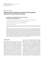
The supernode system corresponds to a global information
transport platform, which consists of a number of heteroge-
neouswirelessnetworks(e.g.,cellularnetworks,MANETs,
wireless local area networks, etc.) that are interconnected
over an Internet backbone [22], as illustrated in Figure 1.
Each wireless access network is connected to the Internet
backbone through a DTN gateway [2]. Each node is able to
connect to the platform through any interconnected wireless
network. To achieve seamless communication for mobile
nodes, the system has a number of supernodes that are
interconnected over the Internet backbone. Each supernode
is responsible for a set of users (mobile nodes), and each
user has a unique and fixed home supernode, independent

of its location changes. The supernodes and the gateways are
assumed to communicate reliably over the Internet. Upon
connecting through any access network, a node contacts
its supernode for registering its current location. To deliver
a message, the source node first locates the supernode of
the destination using the destination ID. With the latest
known location of the destination provided by its supernode,
the source tries to establish an end-to-end connection with
the destination. If the connection fails, all the messages are
sent to and kept at the supernode of the destination for
forwarding to the destination upon its availability. More
details about the supernode system are given in [21].
A dominating-set-based routing scheme is proposed in
[20] for DTN-based MANET routing within the supernode
system. It is based on a dominating set for an established
virtual network topology graph. A dominating set of a graph
is defined as the subset of vertices of the graph where every
vertex not in the subset is adjacent to at least one vertex
in the subset [23]. The virtual network topology graph is
represented as an undirected graph G
= (V,E), where V
represents the set of mobile nodes currently connected to
the network and E represents the set of the estimated contact
probabilities for all node pairs. In the dominating set routing
scheme, message delivery is done by forwarding a message to
the message destination or the dominating set members only.
When a dominating-set member encounters the message
destination, it forwards the message to the destination. The
dominating-set represents the set of nodes that have a high
probability to meet every node in the network; the expected

number of forwarded messages is proportional to the size of
the dominating set.
The main challenge in developing an efficient routing
algorithm for the DTN-based MANET is how to accurately
estimate the probability of a future contact between a pair
EURASIP Journal on Wireless Communications and Networking 3
Roaming user
Cellular
network
Satellite
Wireless LAN
A
DTN
gateway
Router
The
internet
Wireless
ad hoc
network
B
S
C
S
A
S
B
S
D
Figure 1: An illustration of the supernode system.

of nodes, in order to select the best next hop (i.e., carrier)
for the message. In our previous work [20], estimating the
probability of future contact is based on the durations of
node previous contacts which is proved to be more reliable
estimation criterion compared to the criterion of the number
of previous contacts. Without loss of generality, consider
two nodes, A and B.Atanytime,letT
AB
denote the total
time during which nodes A and B were in contact up to
the moment. Regardless of time synchronization and the
time durations during which nodes A and B,respectively,
stay connected to the network, T
AB
= T
BA
. The probability
of a future contact between nodes A and B is estimated
approximately by
P
AB
=
T
AB
[
T
A
+ T
B
]

/2
,(1)
where T
A
and T
B
are the total time durations during which
nodes A and B, respectively, are connected to the network up
to the moment of estimation.
Using (1), a virtual network topology can be constructed
based on network statistics. The topology is represented as
an undirected graph G
= (V, E), where V represents the set
of mobile nodes currently participating in the network and E
represents the set of contact probabilities for all node pairs.
To determine the dominating set, the basic technique for
dominating set calculation proposed in [23]isnotsuitableto
the virtual network topology for two reasons: the first is that
(1) Start with DS contains only the gateway node
(2) for all node i
∈ V and i
/
∈ DS and NG(i)
/
⊆DS do
(3) get max P
ij
where j ∈ NG(i)andNG(j) − i
/
= φ

(4) if j
/
∈ DS then
(5) add j to DS
(6) end if
(7) end for
(8) for all node i
∈ DS do
(9) if j
/
∈ DS, ∀ j ∈ NG(i) then
(10) get max P
ij
where j ∈ NG(i)andj ∈ NG(k)
where k
∈ DS
(11) add j to DS
(12) end if
(13) end for
Algorithm 1: Calculation of the dominating set (DS) based on
previous contact duration [20].
the edge weights should be taken into consideration to select
the most probable nodes to meet and the other is the fact
that the constructed graph may be a fully connected graph
where most of the edges have very low weights which make
the regular algorithm in [23] useless.
Algorithm 1 is proposed in [20] to calculate a dominating
set for the introduced virtual network topology, where DS
represents the dominating set and NG(i) represents the set
4 EURASIP Journal on Wireless Communications and Networking

of neighbors for node i. The procedure for formulating
the dominating set contains two phases. In the first phase,
nodes are processed one by one in ascending order of their
IDs; for each node not already in the set, the node that
is most probable to be met is added to the dominating
set. The second phase ensures that the dominating set is
connected, which is necessary for ensuring the spread of the
message within the set. As the gateway connects the MANET
to the overall system, it should always be included in the
dominating set. A detailed example of how the algorithm can
be applied is given in Section 6.
3. System Model
Consider a MANET that is connected to the supernode
system through a DTN gateway. Within the MANET, nodes
roam freely in a limited geographical area. Any two nodes
are connected when they are able to communicate directly
with each other, that is, when they are within each other’s
transmission range. For simplicity, we assume that all nodes
have the same transmission range and that if a node A can
receive message from a node B then node B can receive
from node A as well. A contact occurs when any two nodes
are connected. We mainly consider mobile nodes to be
sparsely located so that the network is likely to be partitioned
and an end-to-end path between a message source and the
destination rarely exists. As a result, message delivery is
accomplished through the store and forward mechanism in
the DTN framework.
The DTN gateway has a fixed location within the
geographical area, with communication functions and capa-
bilities similar to those of an ordinary mobile node, that

is, the gateway is assumed to have a limited transmission
range and can communicate only with the nodes within
its transmission range. The gateway transmission range
covers only a small geographical area. However, the gateway
has higher processing power and larger buffer space than
mobile nodes. The gateway location within the network
geographical area should be carefully selected in order
to allow the gateway to directly communicate with some
roaming nodes from time to time.
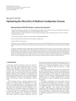
As in real life, users usually have some patterns in
their movements; we consider a Markov-chain-based user
mobility model as in our previous work [20]. Similar
models are also adapted by other researchers such as in
[24]. In this mobility model, the geographical service area
of the MANET is partitioned to m partitions. A node-
to-node direct communication takes place among nodes
within the same partition. Node future location is inde-
pendent of its past location, given its current location.
The residence time of a node in a partition in each visit
is an exponential random variable with parameter λ.For
simplicity, we assume this parameter is the same for all
the nodes and network partitions. Denote the location state
of a mobile node by its current partition. Then, the user
mobility model can be characterized by a one-dimensional
continuous-time Markov chain, with a location state space
given by
{L
1
, L
2

, , L
m
}, as shown in Figure 2.Theuser
movement model over the network coverage area is described
P
L1,2
P
L1,3
P
L1,m
P
L2,m
P
L3,m
···
P
Lm,3
P
L2,1
P
L2,3
P
L3,2
P
L3,1
P
Lm,1
P
Lm,2
S

L1
S
L2
S
L3
S
Lm
Figure 2: Modeling of user movement by a finite-state Markov
chain.
by the transition matrix M of the Markov chain, given
by
M =
⎛
⎜
⎜
⎜
⎜
⎜
⎜
⎝
P
L
1,1
P
L
1,2
P
L
1,m
P

L
2,1
P
L
2,2
P
L
2,m

P
L
m,1
P
L
m,2
P
L
m,m
⎞
⎟
⎟
⎟
⎟
⎟
⎟
⎠
,(2)
where P
L
i,j

is the conditional probability that a mobile
node will enter partition L
j
giventhatitisconnectedto
the network and is leaving its current partition L
i
.Forany
partition L
i
,wehave

j
P
L
i,j
= 1. The transition probability
matrix depends on the geographical characteristics of the
service area and the network environment under study. As
each user may have different preferences for visiting the
network locations, we consider a general case where
M is
unique for each user.
4. Estimation of the Contact Probability
Our goal is to analyze the node mobility model to get
an accurate estimate for the probability of a contact. We
focus on the intermeeting time between two nodes. Define
intermeeting time between a pair of nodes as the duration
from the instant that the two nodes move out of each other’s
transmission range to the instant that the two nodes move
within each other’s transmission range the next time. Define

node interarrival time for a partition as the duration from
the instant that the node departs from the partition to
the instant that the node arrives at the partition the next
time.
In the following, we first study the distribution of
the node interarrival time for a partition and then the
distribution of the intermeeting time.
Theorem 1. The inter-arrival time of a node, A, to a partition,
i, is an exponential random variable with mean 1/λπ
A
i
,where
π
A
i
is the limiting probability in which node A resides in
partition i.
EURASIP Journal on Wireless Communications and Networking 5
Proof. The continuous-time Markov chain for node A is
irreducible. Hence, the limiting probabilities exist, satisfying
the following equations:
π
A
i
=
m

j=1
P
L

j,i
π
A
j
, i = 1, 2, , m,

i
π
A
i
= 1.
(3)
The probability π
A
i
is the fraction of time in which node A
resides in partition i.DefineN(t) as the number of all visited
partitions by time t for node A.Then,N(t) is a Poisson
process with mean λt.DefineN
i
(t) as the number of visits
of node A to partition i by time t. Then N
i
(t) is a Poisson
processwithparameterλπ
A
i
t. As a result, the inter-arrival
time of node A to partition i is exponential with parameter
λπ

A
i
, that is, with mean 1/λπ
A
i
.
Theorem 2 (theory). The intermeeting time between a node,
A,andanothernode,B, is an exponential random variable
w ith mean 1/

m
i=1
2λπ
A
i
π
B
i
.
Proof. Nodes A and B meeting at partition i can occur in
two scenarios: (i) node A moves to partition i while node B
already resides in partition i; (ii) node B moves to partition
i while node A already resides in partition i. Considering
scenario (i), the number of meetings between the two nodes
at partition i is the fraction of node A arrivals to partition i
while node B is residing there. From Theorem 1 and noting
that node B resides in partition i with probability π
B
i
, the

number of meetings between node A and node B at partition
i when node A makes the movement is a Poisson process
with mean λπ
A
i
π
B
i
t. Hence, the intermeeting time between
node A and node B at partition i when node A makes the
movement is an exponential random variable with parameter
λπ
A
i
π
B
i
. Similarly, for scenario (ii), the intermeeting time
between node A and node B at partition i when node B
makes the movement is an exponential random variable with
parameter λπ
B
i
π
A
i
. As a result, the intermeeting time between
node A and node B at partition i is a random variable
that is the minimum of the two independent exponential
random variables, which follows an exponential distribution

with parameter (λπ
A
i
π
B
i
+ λπ
B
i
π
A
i
). Considering all network
partitions, the intermeeting time between node A and node B
is a random variable that has a distribution of the minimum
of the two nodes intermeeting times at all the network
partitions, which is an exponential random variable with
parameter

m
i=1
2λπ
A
i
π
B
i
.
Consider two nodes, A and B.LetP
T

AB
denote the
probability that a contact occurs between A and B,given
that both of them are connected to the network over a
time duration T. The probability of a contact based on the
intermeeting time between the nodes is
P
T
AB
= 1 − e
−

m
i
=1
2λπ
A
i
π
B
i
T
. (4)
(1) Start with DS contains only the gateway node
(2) for all node i
∈ V and i
/
∈ DS and NG(i)
/
⊆DS do

(3) get min E[τ
ij
]where j ∈ NG(i)andNG(j) − i
/
= φ
(4) if j
/
∈ DS then
(5) add j to DS
(6) end if
(7) end for
(8) for all node i
∈ DS do
(9) if j
/
∈ DS, ∀ j ∈ NG(i) then
(10) get min E[τ
ij
]where j ∈ NG(i)andj ∈ NG(k)
where k
∈ DS
(11) add j to DS
(12) end if
(13) end for
Algorithm 2: Calculating the dominating set (DS) based on node
intermeeting times.
To apply the mobility model analysis to the dominating-
set routing scheme, we use the expected intermeeting time
as a measure of link existence, which provides an estimation
of how frequently two nodes will meet in the future.

We construct a virtual network topology as an undirected
graph

G = (V,

E), where V represents the set of mobile
nodes currently connected to the network and

E is the set
containing the expected intermeeting times between any
two nodes. A dominating set for the constructed graph
is calculated using Algorithm 2. Algorithm 2 is a modified
version of Algorithm 1,whereτ
ij
is the intermeeting time
between node i and node j.
5. Dominating-Set Selection
Constraints Relaxation
Increasing the dominating-set size (i.e., number of nodes
in the set) improves the probability of message delivery by
reducing the number of lost (i.e., undelivered) messages, at
the cost of increasing the number of message forwarded.
The extreme case is that the dominating set includes all the
nodes in the network, which corresponds to the epidemic
routing. Selecting dominating-set members based on the
greedy Algorithm 2 does not take into consideration the
dominating-set size, as each node selects the node with
minimum expected intermeeting time. In the following, we
study the problem of reducing the dominating-set size and
propose an alternative dominating-set selection algorithm.

The new algorithm improves the routing performance in
terms of resource utilization, while achieving acceptable
performance in terms of the number of lost messages via an
acceptable average message delivery time.
Message delivery in the system under consideration takes
place when a message carrier comes into contact with the
message destination. For the dominating-set-based routing,
the message carrier can be either a dominating-set member
or the message source itself (i.e., in a case of direct contact).
6 EURASIP Journal on Wireless Communications and Networking
S
τ
S
τ
D
D
···
DS
12
34
N
− 1 N
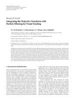
Figure 3: End-to-end message delivery under dominating-set-
based routing.
Assuming a sufficiently large node buffer space, message loss
mainly occurs as a result of the message expiry before a
contact between a carrier and the message destination takes
place. In a regular network, the end-to-end message delay
can be controlled by selecting the message route to enforce
certain quality of service. On the other hand, in a delay-

tolerant network environment, it is so difficult to precisely
estimate the end-to-end delay of delivering a message. Most
research efforts in this problem try to give an estimation for
the delay over a specific route. In [25], it is stated that finding
all the routes from a given source to a given destination
with exact calculation of the expected delay distribution is
an NP-hard problem, where the delay calculation is based
on the primary path that has the smallest expected delay.
To apply this to the dominating set selection problem,
it requires to calculate the shortest path between nodes
for every source and destination. Based on the calculated
shortest paths for all the nodes, the optimal dominating-
set can be selected. Considering network size and dynamics
(i.e., expected change in network memberships due to user
roaming, disconnection, and power failure), the calculations
will be very complicated and impractical.
As shown in Figure 3, where the dominating set has N,
nodes, the message end-to-end delay, denoted by T
D
,for
a no-direct contact case under the dominating-set routing
consists of three delay components: the delay τ
S
for the
message source to deliver the message to the dominating set,
the delay τ
DS
for the message over the dominating set, and
the delay τ
D

to deliver the message from the dominating-set
to the destination node. The expected end-to-end delay can
be expressed as
E
[
T
D
]
= E
[
τ
S
]
+ E
[
τ
DS
]
+ E
[
τ
D
]
. (5)
The delay over the dominating set, τ
DS
,canrangefrom0
in the case of two-hop path delivery to

N−1

i=1
τ
i,i+1
.Note
that τ
i,j
is a random variable that represents the time for
node i to meet node j.Asweassumenocontrolonnode
mobility, the only way to reduce these delay components is
by selecting more nodes in the dominating set. However,
that will increase the number of forwarded messages, which
causes inefficient use of the system resources. Minimizing the
size of the dominating set improves the system performance
in terms of the number of forwarded messages; however,
it increases the number of lost messages as it increases the
expected delivery time. As a tradeoff solution, we propose to
change the dominating set selection criterion from selecting
the nodes most likely to meet with each node in the network
to selecting a minimum set of nodes so that every node in the
network is expected to meet with a member of the set within
a time interval less than certain threshold value θ
t
on average.
Based on Theorem 2 in Section 4, the intermeeting time
between a node, A, and a dominating set member, X,isan
exponential random variable with parameter λ
AX
,givenby
λ
AX

=
m

i=1
2λπ
A
i
π
X
i
(6)
for the network coverage with m partitions.
As a result, the intermeeting time between node A and
the dominating set (excluding A if A is a DS member) is
the minimum of the intermeeting times between A and the
DS members, which is an exponential random variable with
parameter λ
A
,where
λ
A
=

X ∈ DS
X
/
= A
λ
AX
. (7)

Using (5), reducing the expected end-to-end delay can
be achieved by reducing the individual delay components,
such as by reducing the expected intermeeting time between
an individual node and the dominating-set. The newly pro-
posed algorithm, given in Algorithm 3, selects dominating-
set members by including a small set of nodes so that every
node in the network has an expected intermeeting time with
the set less than θ
t
. The algorithm starts with a set, DS,
containing only the gateway node. A node, A, will be added
to DS only if there exists a node B where E[τ
B
] ≥ θ
t
and
E[τ
AB
] = min(E[τ
XB
]), for all X ∈ NG(B), where τ
AB
is the
intermeeting time between A and B, τ
B
is the intermeeting
time between B and DS, and NG(B) is the set of neighbours
for node B. As a result, increasing θ
t
is expected to reduce the

DS size.
Unlike Algorithms 1 and 2, processing a node, A, will
result in adding its most probable node to be met, B,to
the DS, only if the expected time for node A to meet with
a dominating set member does not satisfy the required
criterion θ
t
. The worst case scenario for the new algorithm
is the same dominating set as that from Algorithm 2,fora
very small θ
t
. On the other hand, for sufficiently large θ
t
,
the dominating set may contain only the gateway, which
is similar to the case of direct transmissions. As a result,
the newly proposed algorithm, Algorithm 3,isexpectedto
improve the system performance in terms of the number of
forwarded messages as it can result in a reduced DS, as will
be discussed next.
6. A Network Example
In this section, we consider an example based on a typical
simulation experiment to show how the different algorithms
will process a typical scenario. The network consists of 7
nodes and the gateway S. This network is a fully connected
EURASIP Journal on Wireless Communications and Networking 7
(1) Start with DS contains only the gateway node
(2) for all node i
∈ V and i
/

∈ DS and NG(i)
/
⊆DS do
(3) λ
i
=

X∈DS, X
/
= i
λ
iX
(4) τ
i
= 1/λ
i
(5) if τ
i
<θ
t
then
(6) Skipnextstepsandgetnexti
(7) end if
(8) get min E[τ
ij
]where j ∈ NG(i)andNG(j) − i
/
= φ
(9) if j
/

∈ DS then
(10) add j to DS
(11) end if
(12) end for
(13) for all node i
∈ DS do
(14) if j
/
∈ DS, ∀ j ∈ NG(i) then
(15) get min E[τ
ij
]where j ∈ NG(i)andj ∈ NG(k)
where k
∈ DS
(16) add j to DS
(17) end if
(18) end for
Algorithm 3: Calculating the dominating set (DS) based on
constraints relaxation.
Table 1: Probability of contacts based on previous contact duration
(percentage).
Node ID
SABCDEFG
S —86551075811041
A 86—494957584943
B 5549—7156623338
C 10 49 71 — 49 78 71 84
D 75 57 56 49 — 35 80 25
E 81 58 62 78 35 — 27 91
F 10 49 33 71 80 27 — 37

G 41 43 38 84 25 91 37 —
graph. For presentation clarity, the topology is represented
in a table format, given in Tab le 1 . This table presents the
probability of contact for each pair of nodes in the network
based on the processed statistics of the contact duration
among the nodes. For example, node A has a probability
of 49% to contact node B, when both are connected to the
network, and a probability of 86% to contact the gateway S.It
is important to note that contacts between any pair of nodes
are disjoint events.
Applying Algorithm 1 over the virtual network topology
presented in Table 1, the algorithm starts with a set, DS,
that contains only the gateway S. Processing each node in an
ascending order of node ID, the most probable node to be
met node A is S which is already in DS. For node B, as the
most probable node to be met is node C,nodeC is added
to DS. Node C is not processed as it is already in DS. For
node D,nodeF is the most probable node to be met and
it is added to DS. For node E, the most probable node to
meet is node G,sonodeG is added to DS. Nodes E and
G are skipped from processing as they are members of the
Table 2: Intermeeting time (simulation step).
Node ID
SABCDEFG
S — 41 31 180 35 28 91 77
A 41 —52 49 53406054
B 31 52 — 46 50 50 60 46
C 180 49 46 — 42 46 46 41
D 35 53 50 42 — 40 33 48
E 28 40 50 46 40 — 50 47

F 91 60 60 46 33 50 — 52
G 77 54 46 41 48 47 52 —
selected set. At the end of the first phase, the dominating set
is DS
={S, C, F, G}. The second phase that guarantees the
connectivity of the set is not necessary in this scenario as the
graph is fully connected.
To a p p l y Algorithm 2, it is required to calculate the
expected intermeeting time between each pair of nodes based
on their mobility pattern, which is given in Tab le 2 .Basedon
Ta bl e 2, Algorithm 2 starts with a set, DS, that contains only
the gateway S. Processing each node in an ascending order of
node ID, the resulting DS
={S, E, G, F}, which is a connected
set.
It should be noticed that Algorithms 1 and 2 result in
different sets for the same problem as they process virtual
network topology constructed based on different criteria,
giveninTables1 and 2,respectively.
Reducing the size of the dominating set is the main
design goal for Algorithm 3. This algorithm ensures that each
node in the network has an expected intermeeting time with
the selected dominating set members less than a specific
threshold value. If this cannot be achieved, the algorithm
adds (to the selected set) the node with the least expected
intermeeting time (similar to Algorithm 2).
For the network scenario, assume that message lifetime
= 90 and θ
t
= message lifetime/2. Algorithm 3 starts with

a set, DS, that contains only the gateway S.FornodeA,
τ
A
= 41, so node A will not select any more nodes to be in
DS as τ
A
<θ
t
.FornodeB, τ
B
= 31; similar to node A case,
processing node B will not add any nodes to DS. For node C,
τ
C
= 180, so node C selects the node with the least expected
intermeeting time which is node G to be added to DS. For
node D, where DS
={S, G}, τ
D
= 1/(1/35) + (1/48) =
23.23, so node D will not select any more nodes to be in
DS. For node E, τ
E
= 1/(1/28) + (1/47) = 17.54, so node
E will not select any more nodes to be in DS. For node F,
τ
F
= 1/(1/91) + (1/52) = 33.09, so node F will not select
any more nodes to be in DS. Node G is not processed as it is
already member in DS. The selected dominating set will be

DS
= {S, G}.
It is clear that the new algorithm should result in a
reduced size dominating set given a reasonable value of θ
t
.
Intheextremecaseforverysmallvalueθ
t
, the algorithm
will result in the same dominating set as Algorithm 2.
Section 7 shows how different values of θ
t
affect the routing
performance.
8 EURASIP Journal on Wireless Communications and Networking
It can be seen that all the algorithms for determining
a dominating set for a virtual network topology are based
on the idea of selecting a set of carrier nodes that cover the
whole graph. It is expected that with a smaller dominating
set size, the routing performance will be improved as the
number of forwarded messages will decrease. With a fully
connected network topology, selecting a random set of
nodes can be regarded as an alternative technique. With the
random set selection, there is no actual need for collecting
network statistics and performing dominating set selection
computation, which is expected to reduce the overhead
induced by the link statistics computations. This alterna-
tive technique is evaluated through our experiments in
Section 7.
7. Performance Evaluation

This section presents analytical results in comparison with
simulation results for the inter-arrival time and the inter-
meeting time. Moreover, we evaluate the performance of
the dominating-set-based routing scheme based on the user
mobility model analysis and the newly proposed algorithm
that relaxes the selection constraints. The performance
is compared with that of epidemic routing and of the
dominating-set-based routing scheme using Algorithm 1.
The performance is measured in terms of (i) the numbers
of delivered and lost messages to indicate how reliable each
technique is in delivering messages and (ii) the number of
forwarded messages over the network to demonstrate how
efficiently each technique uses the available resources (i.e.,
radio bandwidth and node buffer space).
In the simulation, the number of partitions of the
MANET coverage area varies in range of 10–50. Each
simulation proceeds in discrete time steps. Mobile nodes
move with mobility trajectories independent of each other.
For each simulation run, the movement matrix
M of each
node is generated at random and stays fixed till the end of
the simulation. Initially, the node locations are uniformly
distributed over the service area. As the simulation time
increases, each node moves randomly according to its
transition matrix. The node residence time at each partition
is an exponential random variable with an average of 10
simulation steps. At the end of the residence time, the node
moves to a new partition based on its mobility matrix.
Messages are generated in the network based on a Poisson
process with mean rate of 910 messages per simulation

time step, with a constant message size. The source and the
destination for each message are selected at random. The
message lifetime is constant with a value of 50 simulation
steps. Each mobile node has a buffer space of 15 messages.
The gateway has a buffer space of 2000 messages. A buffer
overflow occurs when a node buffer is full and a new
message is received. When a buffer overflow occurs, the
oldest message in the buffer is discarded. Message exchanges
occur among nodes residing in the same partition. We
assume that the traveling time between partitions is small
and can be neglected as compared to the partition residence
time. At each time step, the node detects its neighbor
nodes and exchanges the buffered messages with them (the
Table 3: Statistics of the node inter-arrival time.
Partition Simulation Analysis
ID Mean Confidence interval Mean
1 62.59 54.10–71.08 66.25
3 80.54 65.69–95.39 80.63
4 51.83 44.01–59.65 56.36
5 59.57 51.11–68.03 57.04
8 90.64 73.60–107.68 90.59
9 127.44 99.00–155.88 120.04
10 126.58 104.35–148.80 122.12
Table 4: Statistics of the node intermeeting time.
Node Simulation Analysis
pair Mean Confidence interval Mean
1, 2 59.00 49.82–68.18 54.83
1, 3 52.97 45.38–60.55 50.24
1, 4 51.87 44.60–59.14 49.53
2, 3 48.83 41.80–55.87 44.77

2, 4 78.63 62.67–94.59 79.92
3, 4 61.82 50.89–72.75 62.70
messages they do not already have) based on the used routing
technique. For each experiment, a communication scenario
(i.e., set of messages, user connections, user disconnections,
and user movements) is set up randomly and run for each
routing technique. For simplicity of simulation, we assume
that each node can access the medium reliably.
Our first experiment is to validate the distribution of
the inter-arrival time by simulation. In this experiment, we
record node inter-arrival times for different partitions in the
network. The mean and its 95% confidence interval based
on the simulation data are calculated and compared with the
theoretical values based on Theorem 1. It is observed that
the theoretical mean gives a very good approximation to the
simulated data mean, which lies within the calculated 95%
confidence interval of the simulation data. Ta b le 3 shows a
sample of the simulation results for a node moving over a
network consisting of 10 partitions.
Our next experiment is to validate the distribution of the
node intermeeting times by simulation. In this experiment,
we track node-to-node intermeeting times for each pair
of nodes in the network. Ta bl e 4 shows the simulation
results for tracking 4 nodes over a network of 10 partitions
and compares them with the results calculated based on
Theorem 2. It is observed that the simulation and analytical
results match well.
In the following, we study the performance of the
dominating-set-based routing scheme using the node inter-
meeting time as an indication of node-to-node future

contact frequency. The results are obtained by simulating a
network with 20 partitions and 70 nodes.
Figure 4 shows a performance comparison in terms of the
number of delivered messages between the epidemic routing
scheme and the dominating-set-based routing scheme using
both criteria of (i) the intermeeting time and (ii) the duration
EURASIP Journal on Wireless Communications and Networking 9
Epidemic
DS duration
DS intermeeting
300025002000150010005000
Simulation step
10
1
10
2
10
3
10
4
Number of delivered messages
Figure 4: Number of delivered messages under different routing
schemes.
Epidemic
DS duration
DS intermeeting
300025002000150010005000
Simulation step
10
0

10
1
10
2
10
3
Number of lost messages
Figure 5: Number of lost messages under different routing
schemes.
based estimate of the probability of future contacts according
to (1). The dominating-set routing technique based on node
intermeeting times is found to slightly outperform the other
two schemes. This is demonstrated more clearly in Figure 5,
which shows a comparison among the three schemes in
terms of the number of undelivered (lost) messages. With
the node limited buffer space and an increasing number of
exchanged messages, some messages are lost due to buffer
overflow. Using the node intermeeting times as a selection
criterion ensures that message carriers are more likely to
be in contact with the message destination in a shorter
duration. Figure 6 shows a performance comparison in terms
Epidemic
DS duration
DS intermeeting
300025002000150010005000
Simulation step
10
0
10
1

10
2
10
3
10
4
10
5
10
6
10
7
Number of forwarded messages
Figure 6: Number of forwarded messages under different routing
schemes.
of the number of forwarded messages as a measure for the
network resource utilization. It is clear that the dominating-
set routing scheme based on the node intermeeting times
gives the best performance among the three schemes. This
is mainly due to the accurate selection of the dominating
set members that results in a reduced number of forwarded
messages required to achieve message delivery.
On the other hand, experimenting with an increased
node buffer size shows that the three schemes give compa-
rable results in terms of the number of delivered messages
and the number of lost messages (due to a decrease in buffer
overflow). However, the dominating-set routing scheme
based on the node intermeeting times consistently gives
the best performance in terms of the number of forwarded
messages. Considering the inevitability of having a limited

node buffer space, it is clear that a more intelligent buffer
management scheme can improve the performance of the
routing schemes, which is an interesting topic for further
research.
We extend our experiments by implementing the newly
proposed algorithm (i.e., Algorithm 3) for selecting domi-
nating set members based on the criterion of limiting the
expected node intermeeting with the dominating-set to a
threshold value θ
t
. Figures 7 and 8 show the results with
different values of θ
t
,whereθ
1
= Message lifetime/2and
θ
2
= message lifetime/5.
Figure 7 shows how the new algorithm improves the per-
formance dramatically in terms of the number of forwarded
messages as compared to the case of using Algorithm 2
and the case of epidemic routing. Increasing the threshold
value gives better results in terms of forwarded messages but
decreases the performance in terms of the number of lost
messages as shown in Figure 8. It is noticed that Algorithm 3
outperforms Algorithm 2 in terms of the number of for-
warded messages with acceptable performance in terms of
10 EURASIP Journal on Wireless Communications and Networking
Epidemic

θ
t
= θ
1
θ
t
= θ
2
DS intermeeting
300025002000150010005000
Simulation step
10
0
10
1
10
2
10
3
10
4
10
5
10
6
10
7
Number of forwarded messages
Figure 7: Number of forwarded messages under different routing
schemes and different threshold values.

Epidemic
θ
t
= θ
1
θ
t
= θ
2
DS intermeeting
300025002000150010005000
Simulation step
10
0
10
1
10
2
10
3
Number of lost messages
Figure 8: Number of lost messages under different routing schemes
and different threshold values.
the number of lost messages. This is mainly because, under
the new criterion, the dominating set size is reduced.
As Figure 8 shows, the number of the lost message
under Algorithm 3 is larger than that under Algorithm 2.
This is because increasing message holding time at a carrier
node (i.e., DS member) increases the probability that of
message being discarded before being delivered due to a

buffer overflow. With a larger node buffer space, it is noted
that both Algorithms 2 and 3 give comparable results. This is
because message loss in this case is mainly due to the message
expiry, but less likely due to buffer overflow. It is also noted
that, regardless of the buffer space, Algorithm 3 outperforms
Algorithm 2 in terms of the number of forwarded messages.
The threshold value θ
t
plays an important role in the
Epidemic
θ
t
= θ
1
θ
t
= θ
2
DS intermeeting
Random selection
DS duration
300025002000150010005000
Simulation step
10
0
10
1
10
2
10

3
10
4
10
5
10
6
10
7
Number of forwarded messages
Figure 9: The random selection technique performance compared
to the other techniques in terms of the number of forwarded
messages.
Epidemic
θ
t
= θ
1
θ
t
= θ
2
DS intermeeting
Random selection
DS duration
300025002000150010005000
Simulation step
10
0
10

1
10
2
10
3
Number of lost messages
Figure 10: The random selection technique performance compared
to the other techniques in terms of the number of lost messages.
performance based on Algorithm 3. How to determine a
proper θ
t
value, for a given network scenario, requires further
investigation.
Our last experiments investigate the performance of the
random set selection technique (discussed in Section 6),
in comparison with the other techniques, as illustrated in
Figures 9 and 10. The DS size is set to the smallest DS
size from the discussed algorithms, but the DS members
are selected randomly. Figure 10 shows that the random
selection technique degrades the performance significantly
even when compared with the worst performance of the
other techniques. In other words, reducing DS size alone does
EURASIP Journal on Wireless Communications and Networking 11
not improve the performance unless an accurate selection
methodology for the DS members is employed to guarantee
proper contacts between the set members and the other
nodes. The number of lost messages increases due to the lack
of contacts between the set members and the other nodes,
which causes messages to expire before being delivered. This
decrease in contacts also leads to the smallest number of

forwarded messages (as shown in Figure 10)ascompared
to the other techniques. Reducing the number of forwarded
messages in this case cannot be regarded as a performance
improvement because of the significant degradation in the
performance in terms of the number of lost messages.
8. Conclusions
In this paper, we consider the dominating-set-based routing
for a DTN-based MANET within the supernode system. We
analyze the node mobility to better estimate node-to-node
future contact statistics for improving message delivery. The
node intermeeting time distribution is derived based on a
Markovian node mobility model, which is validated by a
simulation study. The node mean intermeeting time is used
in the dominating-set routing scheme. Computer simulation
results demonstrate that the dominating-set routing scheme
based on the node mean intermeeting time outperforms
epidemic routing and dominating set routing based on
previous contact duration, in terms of both message delivery
rate and resource utilization. Moreover, we propose a new
algorithm for selecting the dominating-set based on the
distribution of node intermeeting time, which results in a
smaller dominating-set size. The newly proposed algorithm
chooses a set of nodes so that every node in the network
should have an expected intermeeting time with the set
members under a certain threshold value. The computer
simulation results show the effectiveness of the proposed new
algorithm.
Acknowledgments
This paper was presented in part in IEEE Globecom 2010.
This research was supported by research grants from the

Natural Science and Engineering Research Council (NSERC)
of Canada and from Research In Motion Limited (RIM).
References
[1] H. Samuel, W. Zhuang, and B. Preiss, “Routing over inter-
connected heterogeneous wireless networks with intermittent
connections,” in Proceedings of the IEEE International Confer-
ence on Communications (ICC ’08), pp. 2282–2286, May 2008.
[2] K. Fall, “A delay-tolerant network architecture for challenged
internets,” in Proceedings of the ACM Conference on Computer
Communications (SIGCOMM ’03), pp. 27–34, August 2003.
[3] S. Burleigh, A. Hooke, L. Torgerson et al., “Delay-tolerant
networking: an approach to interplanetary internet,” IEEE
Communications Magazine, vol. 41, no. 6, pp. 128–136, 2003.
[4]P.Juang,H.Oki,Y.Wang,M.Martonosi,L S.Peh,andD.
Rubenstein, “Energy-efficient computing for wildlife tracking:
design tradeoffs and early experiences with ZebraNet,” in Pro-
ceedings of the 10th International Conference on Architectural
Support for Programming Languages and Operating Systems,
pp. 96–107, 2002.
[5] J. LeBrun, C N. Chuah, D. Ghosal, and M. Zhang,
“Knowledge-based opportunistic forwarding in vehicular
wireless ad hoc networks,” in Proceedings of the 61st IEEE
Vehicular Technology Conference (VTC ’05), vol. 4, pp. 2289–
2293, June 2005.
[6] J. A. Davis, A. H. Fagg, and B. N. Levine, “Wearable computers
as packet transport mechanisms in highly-partitioned Ad-Hoc
networks,” in Proceedings of the 5th International Symposium
on Wearable Computers (ISWC ’01), pp. 141–148, October
2001.
[7] A. Doria, M. Uden, and D. P. Pandey, “Providing connectivity

to the saami nomadic community,” in Proceedings of the
2nd International Conference on Ope n Collaborative Design for
Sustainable Development, December 2002.
[8] W. Zhao, M. Ammar, and E. Zegura, “A message ferrying
approach for data delivery in sparse mobile Ad Hoc networks,”
in Proceedings of the 5th ACM International Symposium on
Mobile Ad Hoc Networking and Computing (MoBiHoc ’04),pp.
187–198, May 2004.
[9] Q. Li and D. Rus, “Sending messages to mobile users in
disconnected ad-hoc wireless networks,” in Proceedings of the
6th Annual International Conference on Mobile Computing and
Networking (MOBICOM ’00), pp. 44–55, August 2000.
[10] R. Shah, S. Roy, S. Jain, and W. Brunette, “Data MULEs:
modeling a three-tier architecture for sparse sensor networks,”
in Proceedings of the 1st IEEE International Workshop on Sens or
Network Protocols and Applications, pp. 30–41, 2003.
[11] H. Samuel and W. Zhuang, “Preventing unauthorized mes-
sages in DTN based mobile ad hoc networks,” in Proceedings
of the IEEE Global Telecommunications Conference (GLOBE-
COM ’09), November 2009.
[12] H. Samuel and W. Zhuang, “Preventing unauthorized mes-
sages and achieving end-to-end security in delay tolerant
heterogeneous wireless networks,” Journal of Communications,
vol. 5, no. 2, 2010.
[13] C. E. Perkins and E. M. Royer, “Ad-hoc on-demand distance
vector routing,” in Proceedings of the 10th IEEE Workshop on
Mobile Computing Systems and Applications (WMCSA ’99),pp.
90–100, 1999.
[14] D. B. Johnson and D. A. Maltz, “Dynamic source routing in
ad hoc wireless networks,” in Mobile Computing, vol. 353, pp.

153–181, 1996.
[15] C. E. Perkins and P. Bhagwat, “Highly dynamic destination-
sequenced distance-vector routing (DSDV) for mobile com-
puters,” in Proceedings of the ACM Conference on Computer
Communications (SIGCOMM ’94), pp. 234–244, 1994.
[16] S. Jain, K. Fall, and R. Patra, “Routing in a delay tolerant
network,” in Proceedings of the ACM Conference on Computer
Communications (SIGCOMM ’04), pp. 145–158, September
2004.
[17] I. F. Akyildiz,
¨
O. B. Akan, C. Chen, J. Fang, and W. Su, “Inter-
planetary internet: state-of-the-art and research challenges,”
Computer Networks, vol. 43, no. 2, pp. 75–112, 2003.
[18] A. Vahdat and D. Becker, “Epidemic routing for partially con-
nected ad hoc networks,” April 2000,
/>∼vahdat/ps/epidemic.pdf.
[19] A. Lindgren, A. Doria, and O. Schel
´
en, “Probabilistic routing
in intermittently connected networks,” SIGMOBILE Mobile
Computing and Communications Review, vol. 7, no. 3, pp. 19–
20, 2003.
12 EURASIP Journal on Wireless Communications and Networking
[20] H. Samuel, W. Zhuang, and B. Preiss, “DTN based dominating
set routing technique for mobile ad hoc networks,” in
Proceedings of the International Conference on Quality of Service
in Heterogeneous Wired/Wireless Networks (QShine ’08), July
2008.
[21] H. Samuel, W. Zhuang, and B. Preiss, “DTN based dominating

set routing for MANET in heterogeneous wireless network-
ing,” Mobile Networks and Applications, vol. 14, no. 2, pp. 154–
164, 2009.
[22] H. Jiang, W. Zhuang, and X. Shen, “Cross-layer design for
resource allocation in 3G wireless networks and beyond,” IEEE
Communications Magazine, vol. 43, no. 12, pp. 120–126, 2005.
[23] J. Wu, M. Gao, and I. Stojmenovic, “On calculating power-
aware connected dominating sets for efficient routing in ad
hoc wireless networks,” in Proceedings of the International
Conference on Parallel Processing, pp. 346–354, September
2001.
[24] H. Dang and H. Wu, “Mobility models for delay-tolerant
mobile networks,” in Proceedings of the 3rd International
Conference on Sensor Technologies and Applications (SENSOR-
COMM ’09), pp. 55–60, June 2009.
[25] K. Tan, Q. Zhang, and W. Zhu, “Shortest path routing in par-
tially connected ad hoc networks,” in Proceedings of the IEEE
Global Telecommunications Conference (GLOBECOM ’03), vol.
2, pp. 1038–1042, December 2003.