Quantitative Economics How sustainable are our economies by Peter Bartelmus_8 potx

reserves, we will now enter a new ‘age of transparency’ for share- and stakeholders
(Tapscott & Ticoll, 2003).
9.1.2 Getting Physical or Monetary?
Changing accounting rules and regulations seems to be easier at the national level
as national accountants have some advantages in this regard over their corporate
counterparts: they are less confined by accountancy laws and rules, they are not
directly affected by their own calculations, and their macroeconomic vantage gives
them a broader view and earlier recognition of changing socio-economic priorities.
This may explain why corporate ‘financial’ environmental accounting has lagged
behind national accounting in addressing environmental and human quality-of-life
concerns. On the other hand, environmental ‘management’ accounts (EMA) have
been widely propagated, even at the international level [FR 9.2].
3
However, EMA face the same physical-monetary dichotomy as their national coun-
terparts. Gray (1990, 1992) has been among the first to call for introducing notions like
carrying capacity and capital maintenance into corporate accounts. He recognizes the
value of both physical impact accounting and ‘sustainable cost’ accounting in mone-
tary ‘shadow accounts’. He stops short, though, of advancing an accounting system to
this end, considering the difficulties of doing so ‘monumental’.
Schaltegger and Burritt (2000) tackle the monumental task. In their seminal
book they distinguish between financial (monetary) and ecological (physical)
accounting; they also suggest to ‘take the two together’ in a modular presentation
of an environmental accounting framework. This is indeed similar to the conservative
modular approach of the revised SEEA (United Nations et al., in prep). Schaltegger
and Burrit also adopt a cautious valuation approach,
●
Including only ‘internal costs’ of outlays for environmental protection in the
monetary accounts
●
Assessing environmental impacts through physical input-output accounts
●

‘Integrating’ economic and environmental data by means of eco-efficiency indica-
tors as the ratio of (monetary) value added and (physical) environmental impact.
9.1.2.1 Physical Accounting
Physical accounting of natural resource use and residuals is the most popular way
of meeting stakeholders’ demand for environmental information. Depending on the
scope of the analysis, eco-balances assess the physical environmental impacts of
3
Financial accounts are typically subject to strict legislative regulation to ensure consistent disclo-
sure of the firm’s performance to regulators, investors and stakeholders. Management accounts serve
the internal cost analysis of a firm’s activities according to its particular needs and priorities.
9.1 From Accountability to Accounting 171
172 9 Corporate Accounting: Accounting for Accountability
corporations or local plants, while life cycle analyses focus on product-specific
impacts at different production and consumption stages.
Table 9.1 shows the internationally acclaimed eco-balance of a German cor-
poration
4
as an example of physical input-output accounts. Contrary to conven-
tional input-output systems, the eco-balances also present assets and asset
changes of equipment, buildings and land – the latter with environmental catego-
ries. The flow accounts show material and energy inputs and residual outputs (in
addition to product outputs) – similar to the national material flow accounts
(MFA) (Section 6.3).
Applying impact analysis to a particular product or production process over
the lifetime of the product (from ‘cradle to grave’) is the approach of life cycle
analysis (LCA) [FR 9.3]. Plate 9.1 illustrates the production process of jeans from
Table 9.1 Eco-balance, Kunert AG
Stocks
(12/31/93) Input (1994) Output (1994)
Stocks

(12/31/94)
Stocks
1. Land (sq. m)
a
649,143 12,931 9,602 646,960
1.1 Sealed 68,606 636 2,692 65,750
1.2 Green 448,659 938 340 448,386
1.3 Built-over 131,878 11,357 6,570 132,824
2. Buildings (sq. m)
a
178,473 14,447 17,923 185,369
3. Equipment (piece) 16,542 1,436 1,263 16,715
Flows
4. Materials/products (kg) 1,055,912 8,492,704
4.1 Raw materials 697,183 3,558,124
4.2 Goods 2,082,292
4.3 Auxiliary materials 3,936,325
4.4 Ancillary materials 1,479,171
5. Waste (kg) 2,357,988 36,398
5.1 Hazardous 62,883 3,910
5.2 Other 660,225 32,488
6. Energy/waste heat (kWh) n/a 118,986,313 118,986,313 n/a
7. Water/waste water (cu. m) n/a 428,770 339,277 n/a
8. Air emission (kg) n/a n/a
8.1 NO
x
100,548
8.2 SO
2
170.132

8.3 CO
2
36,109,594
8.4 Steam 96,895,400
Note:
a
Imbalances in stocks 1993/1994 are due to improved data collection in Tunisian and
Moroccan factories.
Source: Kunert AG (1994/1995, pp. 14/15).
4
In 1995 the Kunert AG’s environmental report was chosen as the ‘world-best’ by SustainAbility
Ltd., a London-based research institute, on behalf of the United Nations Environment Programme.
the production of cotton to the use and disposal by consumers, with recycling
loops back to the consumers as second-hand goods or to reprocessing in cloth
manufacture. Detailed analyses could and should assess the environmental
impacts at all stages of production and transport, especially with regard to emis-
sions and fuel use.
Physical accounting faces of course the problem of comparing the significance
of impacts assessed in different measurement units. As in the MFA, the closest
physical corporate accounts can come to combining environmental impacts with
economic output are resource productivity or eco-efficiency ratios. At the same
time, the detail and knowledge available at the micro-level of the enterprise permit
a more valid intuitive evaluation of environmental impacts than at the national level.
However, full integration is possible only by costing environmental impacts in
monetary accounts.
9.1.2.2 Monetary Accounting
On the monetary side of corporate environmental accounting, the less problematic
assessment of internal environmental protection expenditures has made greater
Plate 9.1 Life cycle of jeans
Copyright VisLab/Wuppertal Institute for Climate, Environment and Energy; with permission by

the copyright holder (See Colour Plates).
9.1 From Accountability to Accounting 173
174 9 Corporate Accounting: Accounting for Accountability
strides than the valuation of environmental externalities. It is clearly more attractive
for a firm to present its environmental protection efforts than to cost its impact on
the outside world. Vividly put: ‘who could expect turkeys to vote for Christmas?’
(Bebbington et al., 2001).
It is no surprise that calls for assessing and internalizing the full (private and
social) costs of the corporation’s activities come typically from policymakers. Their
expectation is that voluntary initiatives by the private sector might obviate unpopu-
lar market interventions such as eco-taxes or regulations (see Ch. 13). Agenda 21
of the Rio Earth Summit urges ‘governments, business and industry … [to] work
towards … the internalization of environmental costs into accounting and pricing
mechanisms’ (United Nations, 1994, ch. 30). Under the heading of ‘getting the
prices right’, the EU’s Fifth Environmental Action Programme called for the
‘redefinition of accounting concepts, rules, conventions and methodology’ for full
environmental cost accounting (European Commission, 1993). Not much progress
seems to have been made since then, except, possibly, when considering accounting
for emission rights and emission prevention as assets and liabilities under the EU
Emission Trading Scheme (Casamento, 2004). Still, professional associations in
the UK and North America elaborated the concepts and methods of full-cost
accounting, possibly in anticipation of further governmental regulation [FR 9.2].
9.1.3 Micro-Macro Link
The national accounts are based on double-entry bookkeeping of enterprises.
Micro-level corporate accounting that is fully consistent with aggregate national
accounting would facilitate statistical data compilation. It would also support
economic analysis, in particular of the distribution of income and wealth. One of
the SNA handbooks thus explores the relationships between micro- and macro-
accounts (United Nations, 2000b). The handbook also reveals numerous differ-
ences in accounting concepts, procedures and indicators such as depreciation by

firms (for tax purposes) and capital consumption in the national accounts (for
assessing the wear and tear of fixed capital).
5
Despite these differences, corporate environmental accounting takes approaches
that are similar to the greening of the national accounts. They include, in particular,
●
Corporate ‘parallel’ or ‘shadow’ accounting for externalities (Bebbington et al.,
2001), comparable to the SNA’s satellite accounts for the SEEA
5
As the national accounts record transactions between different economic agents, they frequently
expand double-entry accounting (for internal production and financial flows) of enterprises into
quadruple-entry accounting, adding the same transaction for buyers and sellers (United Nations
et al., 1993). The SNA also describes the micro-macro links between business and national
accounting and underlying economic theory.
●
The dichotomy of physical vs. monetary accounting in physical eco-balances
and full-cost accounts
●
The segregation of environmental protection expenditures from corporate
overhead costs, and from the SNA’s economic activity classifications in
the SEEA.
Corporate and national accountants could indeed learn from each other about
their respective methods and the use and usefulness of harmonized green
accounting at micro-, meso- and macro-levels. The benefits of this micro-macro
link would be
●
Enhanced compatibility of physical material flow and monetary environmental
cost accounts at enterprise, household, regional and national levels
●
Consistent micro- and macroeconomic strategies and policies, addressing the

sustainability of production and consumption patterns of economic sectors, cor-
porations and households, and of the overall economic development of regions
and countries
●
Identification and measurement of critical capital maintenance, the key ingredi-
ent of strong sustainability (cf. Section 8.4.1), notably through LCA and with a
view to exploring aggregation at sectoral and national levels
●
Improved quality of aggregated environmental stock (ledgers, assets) and flow
(input, output) data from harmonized data sources.
The integrated – physical and monetary – accounting system of the SEEA appears
to provide the best available framework for further developing the micro-macro
link in the fields of environmental-economic accounting and analysis.
9.2 From Accounting to Management
Corporate environmental accounts provide direct data input for corporate environ-
mental management. However, the main international management guidelines of
the ISO (International Organization for Standardization) 14000 and the European
Union’s EMAS (Environmental Management and Audit Scheme) [FR 9.3] do not
clearly link environmental accounting and management. Some connections can be
envisaged, though, between accounting data and performance indicators proposed
by ISO and EMAS for environmental management. Both management guidelines
categorize these indicators as
●
Operational performance indicators of material inputs and outputs
●
Management performance indicators of programme costs, and internal safety
and health
●
Environmental condition indicators of environmental quality and effects on
human health and other socio-cultural amenities.

Based on these indicators ISO and EMAS suggest internal and external audits for
the evaluation of environmental performance. Such audits serve the information
9.2 From Accounting to Management 175
176 9 Corporate Accounting: Accounting for Accountability
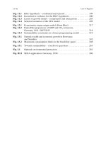
Fig. 9.1 ISO 14000 standards for environmental management
Source: Based on Wohlfahrt (1999).
needs of stakeholders and the improvement of environmental management in the
organization. Figure 9.1 depicts a cycle of continuous performance evaluation and
improvement for the ISO 14000 series with an indication of more specific recom-
mendations (by numbers of ISO standards). The company’s environmental policy,
planning and measures form its ‘environmental management system’ (EMS). The
evaluation of the EMS by performance indicators and audits may warrant further
improvement in environmental management, possibly changing environmental policy.
The basic goal of this cycle is to encourage organizations to move from reactive
treatment of environmental damage to proactive damage prevention.
ISO 14000 and EMAS are quite similar in their scope and coverage, owing to
the incorporation of ISO 14001 (‘Environmental Management Systems –
Specifications with Guidance for Use’) into the revised EMAS II. There remain,
however, important differences, in particular
●
The regional validity: EU member states for EMAS, and worldwide coverage
for ISO 14000
●
An environmental ‘declaration’ under the authority of the EU vs. a less specific
environmental ‘policy statement’ proposed by the non-governmental ISO
●
The EMAS logo, which can be used on-site and on stationary, but not for prod-
uct advertising (Plate 9.2).
The global scope and the less stringent supervision of ISO explain its greater popu-
larity: as of January 2007 there were 129,031 ISO certifications as compared to

5,389 for EMAS.
6
6
/>Both guidelines are voluntary. Despite the clamorous advocacy of corporate
social responsibility, they found only limited application. It remains to be seen whether
actual or perceived economic benefits of environmental management will foster
greater use, notably by small and medium-sized enterprises. Like the United
Nations programme of environmental management accounting (Section 9.1.1), the
ISO and EMAS management guidelines advertise their benefits as
●
More efficient environmental management
●
Natural resource (cost) savings
●
New business opportunities and innovations
●
Reduction of liabilities for environmental hazards
●
Improved staff-management relations
●
Better credit conditions and credibility
●
Improved image of the corporation.
Catering to a broad notion of CSR, a coalition of business, accountants, investors
and stakeholders advanced further guidelines on sustainability reporting. The
Global Reporting Initiative (GRI) aims to extend environmental performance evalu-
ation and reporting, covering contributions to all three dimensions of sustainable
Plate 9.2 EMAS logo
Source: with permission by the
copyright holder, Stora Enso Kabel Mill, Germany (See Colour Plates).

9.2 From Accounting to Management 177
178 9 Corporate Accounting: Accounting for Accountability
development. To this end, the GRI also presents economic, social and environmen-
tal performance indicators [FR 9.3].
Further Reading
FR 9.1 Corporate Social Responsibility
The World Business Council for Sustainable Development seeks to bring about sustain-
able development through eco-efficiency, innovation and corporate social responsibility
(CSR) ( />Id=NjA&doOpen=1&ClickMenu=LeftMenu). Agenda 21 of the Rio Summit promotes
‘cleaner production’ by full-cost pricing, life cycle analysis and ‘responsible entrepre-
neurship’ (United Nations, 1994, ch. 30). The Secretary General of the United Nations,
after addressing the World Economic Forum in 1999, launched a Global Compact of
United Nations agencies, business, labour and civil society to take stakeholder concerns
into account through ‘responsible corporate citizenship’ ( />global.htm). The Johannesburg Summit (United Nations, 2003) stresses in its Political
Declaration ‘the duty’ of companies ‘to contribute to the evolution of equitable and
sustainable communities and societies’ and the ‘need … to enforce corporate accounta-
bility’. Its Plan of Implementation promotes ‘corporate responsibility and accountabil-
ity’, among others through ‘public-private partnerships’. The European Union developed
a European Strategy on CSR, whose ‘centerpiece’ is the European Multistakeholder Forum.
The Forum is to promote ‘transparency and convergence’ on CSR (.
int/comm/enterprise/csr/index_en.htm).
The Journal of Corporate Citizenship presents special theme issues on the theory
and practice of CSR. The CSR Newswire is a source for ‘press releases, reports and
news’ on corporate responsibility and sustainability ( />FR 9.2 Environmental Management Accounting
and Full-Cost Accounting
The United Nations organized a series of workshops to assess governments’ role
in promoting Environmental Management Accounting (EMA) (.
org/esa/sustdev/sdissues/technology/estema1.htm). The United Nations also
surveyed national and international EMA efforts, recommended exploring the rela-
tionships of environmental management systems and national green accounting

(United Nations, 2002a), and advanced material flow costing in terms of ‘wasted
material purchase value’ (quite different from environmental costing in the SEEA)
(United Nations, 2001a). The Environmental Management Accounting Research
Center provides a web site on the US EPA Environmental Accounting Project and
offers links to international activities and networks (
The Environmental Management Accounting Network (EMAN), an EU-sponsored
forum for sharing information about EMA, intends to focus on ‘sustainability
accounting’ in its future publications ( />The British Association of Chartered Certified Accountants (ACCA) published
a comprehensive study on ‘full cost accounting’ (Bebbington et al., 2001), follow-
ing a call for environmental cost internalization by the EU’s Fifth Environmental
Action Programme ( The
2004 ACCA report (
seems to be more pessimistic about implementing the ‘holy grail’ of full-cost
accounting; it still sees an opportunity for liability accounting in the context of the
EU’s emission trading scheme (Casamento, 2004 in ch. 4). The Canadian Institute
of Chartered Accountants (1997) and the Center for Waste Reduction Technologies
(1999) advanced similar proposals.
FR 9.3 Environmental Management and Reporting
The following web sites present the two main international environmental manage-
ment guidelines:
ISO 14000: />html and the EU Environmental Management and Audit Scheme (EMAS): http://
europa.eu.int/comm/environment/emas/index_en.htm. The ISO guidelines (ISO
14040-43) incorporate life cycle analysis (LCA). UNEP promotes LCA in its life
cycle ‘assessment’ and ‘initiative’ (
The World Resources Institute provides a concise overview of LCA: http://www.
gdrc.org/uem/lca/life-cycle.html.
The Global Reporting Initiative (GRI) ( />brief.asp) could be seen as a direct application of the communication module of
environmental management (Fig. 9.1). There are no explicit links, however, to ISO
14000 and EMAS. Part C of the GRI’s ‘Sustainability Reporting Guidelines 2002’
contains a detailed description of sustainability performance indicators: http://

www.globalreporting.org/guidelines/2002/contents.asp.
Review and Exploration
●
Should corporations get involved in improving the social and environmental
conditions of their neighbourhood communities?
●
Why should business account for external effects of its activities?
●
Describe the benefits of the micro-macro link in green accounting.
●
Compare the scope, coverage and contents of ISO 14000 and EMAS II.
●
Do environmental accounting and management improve the bottom line (profits)
of corporations?
Review and Exploration 179
Part IV
Analysis – Modelling Sustainability
Applied mathematical models can combine eco–nomic theory, sketched out in
Chapter 2, with suitable measurement as presented in the green accounting systems
of parts II and III. As a result, applied models could
• Explain the complex environment-economy interaction transparently, rather
than intuitively, and
• Predict environmental impacts for formulating policy options.
Inevitably, modelling entails some abstraction from real-world complexities. In order
to minimize this information loss, part IV focuses on those models and techniques
that are closely related to the accounting systems, i.e. input-output analysis.
Computerized models can handle vast amounts of economic and environmental
variables and their complex interrelationships. Measurability and data availability
pose limits, however, to representing reality with reasonable accuracy. Several mod-
els in this part take, in fact, CO

2
emission as a convenient surrogate for environmental
impacts. Green accounting case studies do indicate a heavy burden from, and consid-
erable mitigation cost of, this greenhouse gas.
1
However, as discussed in section 4.3,
such a reductionist view carries the risk of distorting the significance of environmen-
tal concerns themselves and their role in sustainability analysis. The presentation of
CO
2
-focused models in this part serves, therefore, mostly illustrative purposes; it also
points to the need for better coverage of environmental impacts.
Chapter 10 reviews first the results of sustainability measurement obtained from
the physical and monetary accounts. It enters ‘analysis’ by transforming the supply
and use accounts of the national accounts into input-output tables. Input-output and
related techniques permit tracing the full, direct and indirect, environmental
impacts of different economic activities and identifying the main driving forces
behind these impacts. Chapter 11 moves from descriptive to predictive analysis.
1
For instance, hybrid accounts in the Netherlands showed the weight of CO
2
emission to exceed
the weight of all other pollutants by several orders of magnitude (Section 7.3, Table 7.2). In
Germany, half of the pollution cost, which makes up the bulk of environmental cost, stems from
CO
2
emission (at a 25% reduction standard: see Annex III).
The chapter also explores econometric and simulation techniques in two applica-
tions that test the connection between economic growth and environment at
national and global levels. Chapter 12 turns then to more prescriptive models,

which seek to show how sustainability and optimality can be reconciled in eco-
nomic policy analysis.
182 Analysis – Modelling Sustainability
Chapter 10
Diagnosis: Has the Economy Behaved
Sustainably?
The title question of this chapter cannot be answered unequivocally. Economic welfare
measures may refer to the ultimate goal of economic activity. However, they suffer
from problems of measuring the utility of economic benefits and the disutility (dam-
age) from environmental impacts. Material flow indicators are more specific: they
indicate that the relatively strong sustainability concept of dematerialization is still
an elusive goal, nationally and globally. Green accounting case studies show weak
sustainability for most economies, with some exceptions, notably of African coun-
tries which appear to live off their produced and natural capital base.
Tracing the total, direct and indirect, environmental impacts of economic activi-
ties and their driving forces is the task of input-output and decomposition analyses.
To date, such studies are still isolated efforts, dealing with selected pollutants or the
usual environmental placeholder of CO
2
emission.
10.1 Welfare Secured? Dematerialized? Capital Maintained?
10.1.1 Welfare Indices: Confirming the Threshold Hypothesis?
The closest economists have come to measuring welfare is by adding or deducting
selected (quantifiable) effects on human well-being to/from utility-generating personal
consumption or income. Time series of indices such as the Measure of Economic
Welfare (MEW), the Index of Sustainable Economic Welfare (ISEW) or the Genuine
Progress Indicator (GPI) supposedly indicate past and, by extrapolation, future trends
of economic welfare generated by production and consumption (Section 7.1.1). A
persisting decline of national welfare would indicate the non-sustainability, at least
for the period covered, of the outcomes of economic activity.

An opening-scissor trend of GDP and the welfare indices provides the main evi-
dence – at least for ecological economists
2
– for non-sustainable economic growth
2
For example, Friends of the Earth: see also
Costanza et al. (1997a), Sachs et al. (1998), and Daly and Farley (2004).
P. Bartelmus, Quantitative Eco-nomics, 183
© Springer Science + Business Media B.V. 2008
184 10 Diagnosis: Has the Economy Behaved Sustainably?
Fig. 10.1 ISEW and GDP: No threshold in Italy?
Source: />that undermines the human quality of life. Methodological and data problems
render the validity of this evidence questionable. Moreover, actual index compila-
tions (cf. Fig. 7.2) do not generally support the ‘threshold hypothesis’ (Max-Neef,
1995) of gaping trends of welfare and economic growth, once a certain level of
growth is reached. Contradictory interpretations of these indices might stem from
short time series available after the presumed turning points, preventing any mean-
ingful extrapolation of trends. Figure 10.1 exemplifies for Italy that the ISEW cal-
culation does not provide the distinct scissor movement observed in the USA.
Replacing monetary valuation by averaging physical indicators in indices of the
quality of life, well-being or sustainable development blurs the meaning of the
indices by weighting equally unequal concerns; it also loses comparability with
measures of economic performance (Section 5.3). As a consequence, these indices
do not attempt to assess the sustainability of economic growth. Rather, they com-
pare relative ‘sustainability’ in country rankings or show well-being scores only.
The ‘sustainability barometer’ is deemed to be an indicator of such well-being; it
sets a quite arbitrary sustainability level of 80 points (out of 100) and claims that
no country has achieved this level (Section 5.2).
All in all, it does not seem to be possible to assess the (non)sustainability of
economic growth with opaque measures of economic well-being (welfare) or the

human quality of life.
10.1.2 Dematerialization: Delinkage of Economic Output
and Material Input
Material flow accounts have distinct systemic advantages over ad hoc attempts at
aggregating indicators by averaging or other types of weighting. The reason is that
they base the measurement of material and energy flows on thermodynamic theory.
Still, besides equal weighting of unequal environmental pressures, physical mate-
rial aggregates are not directly comparable with economic indicators. The compari-
son of material flows and economic indicators resorts therefore to comparing their
speed rather than their levels.
The result is the assessment of sustainability as a matter of decoupling the material
indicators, notably total material input, from GDP. The questions are then: how much
decoupling do we need, and for how long? On their own, material inputs may capture
actual and potential pressures on national or global carrying capacities. Assessing
sustainability has to go farther, however, by setting a standard for the maximum per-
missible pressure on environmental source and sink functions. Measuring the eco-
logical sustainability of economic growth becomes thus distinctly normative.
The popular Factor 4 standard uses the relatively opaque notion of available
‘environmental space’ to defend its call for halving material inputs into the planet’s
economies. A more cautious but at the same time fuzzier approach reduces the
Factor 4 or 10 standards to safe guardrails guiding development, rather than
prescribing precise targets (cf. Section 2.4.2).
10.1 Welfare Secured? Dematerialized? Capital Maintained? 185
186 10 Diagnosis: Has the Economy Behaved Sustainably?
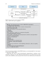
Figure 10.2 indicates that, at least in Germany, economic performance is still
far away from halving material inputs (from levels in the 1990s), and the outlook
for getting there does not look good. Clearly, from an ecological sustainability
point of view, this economy, just as those of most other industrialized countries
(see Section 6.3.2), has not behaved sustainably over the last 40–50 years. The
EU strategy on the sustainable use of natural resources comes to the same conclu-

sion, pointing out that material consumption has remained constant over the last
20 years. At the same time, the strategy rejects setting quantitative targets due to
lack of knowledge and indicators (Commission of the European Communities,
2005).
10.1.3 Capital Maintenance: Has Economic Growth
Been Sustainable?
Greening the national accounts achieves comparability of environmental impacts
with economic indicators by costing the impacts as natural capital consumption.
The economic sustainability notion of capital maintenance calls for reinvesting the
cost allowance for capital maintenance (Sections 2.3.1, 8.2.1). Industrialized coun-
tries and many developing ones increased their capital base through truly net capital
formation – net of produced and natural capital consumption (Section 8.3). However,
a significant number of nations, mostly from Africa, seemed to have lived off their
produced and natural capital base, if the rough World Bank estimates can be trusted
0
5000
10000
15000
20000
25000
30000
35000
40000
45000
50000
GDP per capita (Deutsche Mark)
TMR per capita
Factor 2
Factor 10
GDP per capita

?
?
?
0
10
20
30
40
50
60
70
80
90
100
TMR per capita (tonnes)
1960 1970 1980 1990 2000 2010 2020
Fig. 10.2 Is Germany’s economy sustainable?
Notes: 1960–1990 Federal Republic of Germany (West), 1991–1996 Federal Republic of
Germany; TMR compiled by the Wuppertal Institute for Climate, Environment and Energy; GDP
in 1996 prices.
(see Table 8.2). Of course, maintaining the total value of capital is only a necessary
condition for weak sustainability of economic growth, ignoring critical natural
capital and the role of other human and social capital categories.
Conventional economic net indicators of value added, domestic product and
capital formation overstate economic performance with regard to the social (envi-
ronmental) costs generated during the accounting period. A more accurate reckon-
ing of these costs reveals the necessary economic effort that should and could have
been made for replacing, avoiding or reducing the natural capital loss during the
accounting period. Amounting to a few percentage points of NDP (Table 10.1),
these environmental costs are well within the reach of industrialized countries.

Developing countries, on the other hand, seem to face relatively high costs of natu-
ral resource depletion. At the same time, many developing countries are endowed
with significant natural resources. Rent (profit) absorption and reinvestment by
government might be the crucial way of fostering their economic development,
rather than relying on fickle aid and debt relief (Section 13.3.2).
Asset accounts, including environmental assets, are a more forward-looking tool
of assessing capital maintenance. The availability of produced and natural capital
indicates economic growth potential. However, measurement and valuation prob-
lems of different types of produced capital stocks, natural resource deposits (rang-
ing from speculative to proven reserves) and a large variety of environmental sinks
have prevented so far the regular compilation of these stocks in the national and
environmental accounts. Section 7.1.2 showed the flaws of an attempt at compre-
hensive wealth measurement; it also stressed the importance of wealth for future
economic growth and development.
In principle, asset accounts include the ‘other asset changes’ of natural and politi-
cal disasters, discoveries, regrowth and revaluation. Contrary to exhaustible natural
capital that is lost in destructive disasters, produced capital can be reproduced. The
write-off of disastrous capital loss as economic disappearance under other asset
changes does not affect national product and income, but a remedial increase in
public and private capital formation does. As a consequence, the full (social and
economic) cost of wars and natural disasters are generally underestimated overstat-
ing the net economic ‘stimulus effect’ of such events.
Table 10.1 Environmental depletion and degradation cost in selected countries (% of NDP)
Developing countries Industrialized countries
China 6 Germany 3–4
Costa Rica 4–11
a
Japan 2–3
Ghana 17–25 Korea, Republic of 2–4
Indonesia 13–31

a
UK 0–5
b
Papua New Guinea 3–10 USA 0.4–1.5
c
Philippines 0.5–4
a
Notes:
a
Depletion only.
b
Oil and gas depletion only.
c
Subsoil resources only.
Source: Table 8.1.
10.1 Welfare Secured? Dematerialized? Capital Maintained? 187
188 10 Diagnosis: Has the Economy Behaved Sustainably?
To answer the question of this chapter: most nations show weakly sustainable
growth, with notable exceptions in the poorest countries. These countries did not
have the means to reserve enough resources for capital maintenance, unable even
to replace the wear and tear of produced capital. On the other hand, if we accept the
normative Factor 4/10 targets, we may safely conclude that nearly all countries are
still far away from relatively strong sustainability of economic growth.
Further analysis is needed to predict whether there is a good chance of reaching
these targets within the next few decades as proclaimed by the Factor 4 stipulation.
The following sections discuss first the analytic techniques that can reveal the full
(direct and indirect) environmental impacts of different economic activities, as well
as the driving forces behind these impacts. The next chapters will then extend these
tools into examining future trends and policy scenarios.
10.2 What Are the Causes? Structural Analysis

of Environmental Impact
Figure 10.2 connects the aggregate analyses of the physical MFA and the monetary
SNA accounts. By plotting the time series of TMR and GDP next to each other the
figure represents the overall outcome of hybrid accounting. Extrapolation of these
indicators might or might not show (as indicated by different arrows in the figure)
a sufficient dematerialization of future economic growth, and hence its potential
ecological sustainability.
This section turns from the bird’s-eye view of the economy and environment to
the ground of structural analysis. The objective is to find which sectors and driving
forces are responsible for environmental impacts. Three basic approaches can be
distinguished:
●
Comparison of sectoral economic performance with direct environmental
impacts in environmental-economic profiles
●
Modelling of direct and indirect impacts from economic activities by means of
input-output analysis
●
Time-series analysis of the driving forces behind environmental impacts by
means of structural decomposition.
The value of such analyses depends crucially on meaningful aggregation and disag-
gregation of environmental impacts. However, weighting and valuation problems
render most structural analyses of environmental concerns highly selective: typically
they deal with one (notably CO
2
) or selected pollutants only. The revised SEEA
defends the ‘legitimacy’ of selecting ‘the most urgent environmental concerns’ in
hybrid accounts as building ‘a bridge between (aggregate) policy assessment and
(underlying) policy research’ (United Nations et al., in prep.). The structural flaw of
this bridge is that selectivity adds a further assumption of ‘representativity’ for total

environmental impact to the difficulties of comparing physical and economic indica-
tors. Anticipating the building of safer bridges, which can carry the full load of
environmental impacts, this section reviews briefly the use of hybrid accounts and
input-output analysis in assessing selected pollutants from economic sectors.
10.2.1 Environmental-Economic Profiles
Hybrid accounts are a good starting point for generating ‘environmental-economic
profiles’ (United Nations et al., in prep.). The profiles compare directly the sectoral
contributions to GDP with their share of natural resource inputs and residual outputs.
They also give a first indication of the structural causes for environmental impacts and
of possible trade-offs between economic benefits and environmental deterioration.
The aggregated Table 10.2 describes in the first column Germany’s post-industrial
economy, where the service sector accounts for over two thirds of the value added
generated in all production sectors. At the same time, the industrial sector of mining,
manufacturing, construction and utilities is responsible for the bulk of environmental
deterioration. As usual, CO
2
emission in column 2 may stand for environmental deg-
radation. A further breakdown by industries reveals a similar pattern, with the energy
sector contributing 2% to GDP but accounting for 40% of CO
2
emissions.
Table 10.2 presents energy and pollution intensity, abstracting from the level of
economic activity by showing the environmental effects of production and con-
sumption patterns. Generally, CO
2
emission intensity has declined since 1991. On
the other hand, the large variation of both energy and pollution intensities among
economic sectors indicates that environmental impacts are not only a matter of
scale but also of structure. Section 10.2.3 attempts to quantify and compare these
influences of structure and level. But first, let us explore the impact side of eco-

nomic activity in greater detail.
Table 10.2 Environmental-economic profiles: Energy and CO
2
intensities, Germany 2000 (1991)
Gross value
added
a
(%)
CO
2
emission
(%)
Energy consump-
tion per gross
value added
a
(Mj/C
=
)
CO
2
per gross
value added
a
(kg/'000 C
=
)
2000 1991
(1) (2) (3) (4) (5)
Agriculture, forestry,

fishery
1.3 1.0 5.8 350 581
Mining, manufacturing,
construction, utilities
29.6 62.8 15.3 1020 1,194
Services 69.0 13.2 1.7 92 106
Total
industries
100 (76.9) 5.8 370 489
Domestic private
consumption
23.1 3.6 188
b
240
b
Grand Total 100
Notes:
a
1995 prices.
b
CO
2
emissions per private household consumption in constant prices.
Source: Statistisches Bundesamt (2002, data from Annex Tables 18, 26, 34, 37).
10.2 What Are the Causes? Structural Analysis of Environmental Impact 189
190 10 Diagnosis: Has the Economy Behaved Sustainably?
10.2.2 Direct and Indirect Impacts: From Accounting
to Modelling
The basic assumption of input-output analysis [FR 10.1] is, quite realistically, inter-
dependence of different industries. Each industry may thus provide, in principle,

inputs to all other industries. In this case it is not sufficient to measure only the
immediate environmental impact from using a specific set of inputs in the production
of a particular product. Rather, for an assessment of the total impact of a product, one
would have to assess all the impacts resulting from the full chain of different inputs
used – not only in the last-stage production process but also in all ‘antecedent’
industries.
Classic input-output analysis determines the total amount of an output x
i
required
for delivering final goods and services in an inter-industry exchange system. A
‘squared’ input-output table with fixed-coefficients linear production functions
facilitates standard input-output analysis.
3
The inclusion of environmental impact
generation activities, which use economic products as the ‘inputs’ into the impact
process, allows then determining the full – directly and indirectly – generated
impact per unit of a particular output, sector or the economy.
For example, the set of Equations (10.1) presents an n-product x
i
(i = 1,2…n)
and one-pollutant p production system, with given final demand y
i
, a set of fixed
input a
ij
and pollution a
pj
coefficients (j = 1,2…n), and the – unknown – total
amount of pollution y
p

generated by this system. Equation (10.2) is the solution of
this system for all outputs x, with (I – A)
−1
(the inverse of the direct coefficients
matrix A) representing the matrix of total (direct and indirect) production and pol-
lution coefficients:
(1
+
−−−−=
−−−−=
≡−
ax ax ax y
ax a x ax y
1122 1nn1
21 1 22 2n n 2
11
2
)
()
…
…

1
xAxy=
(10.1)
−−−+− =
−++=
=
−
ax ax a x y

ax ax ax y
(- )
n1 1 n2 2 n n
p1 1 p2 pn n p
…
…
(1
+
nn
2
)
xIA
11
y
(10.2)
3
Solving the equations of an input-model model by calculating the inverse matrix of its input-
coefficients requires a squared input-output table. Typically, squaring needs to be done when
using the supply and use tables (SUT) of the national accounts as the database for input-output
tabulations. The SUT are usually rectangular, since they combine an unequal number of indus-
tries and products. Converting industries into products or bundling products into industries to
equalize the numbers and rows of the input-output system requires considerable estimation and
data ‘manipulation’ (United Nations et al., in prep.).
Figure 10.3 compares the inverted (total) pollution coefficients A
pj
with the
direct pollution coefficients a
pj
for selected industries and one particular pollutant,
p (CO

2
). Based on a hybrid input-output table, the coefficients show CO
2
emission
per million Swedish krona (SEK) of output. The differences between direct and
total emissions are particularly high in transport, energy, paper and water industries.
Note that for water supply and treatment there are no direct emissions, and the total
stems thus from emissions embodied in the traced-back input chain. The A
pj
are
calculated for a closed economy; they represent therefore the emissions from
domestic production and final use only. For an open economy such as Sweden’s one
should calculate the additional emissions generated by the production chain of
imported goods in order to reflect the responsibility of domestic final demand for
emissions generated not only at home but also abroad. Figure 10.3 indicates that the
inclusion of imported petroleum products is responsible for a particularly high
increase in CO
2
emissions from domestic demand for foreign products.
Assuming a fixed-coefficient homogeneous production function with constant
returns to scale for each industry (the classic Leontief assumptions) is the smallest
but nonetheless definite transition from descriptive accounting to modelling. The
transition is small because it retains the observed technical coefficients as model
parameters (unless obtained from data ‘manipulation’ when squaring the supply/
use table). Emissions, generated in a ‘whirlpool’ (Dorfman, Samuelson & Solow,
1958) of preceding production processes, might lead back into past accounting
periods when inputs were actually produced and used. It is far from obvious that
Fig. 10.3 Direct and total CO
2
emission coefficients, Sweden 1991

Source: Hellsten et al. (1999), table 9, p. 63; with permission by the copyright holder, Elsevier.
10.2 What Are the Causes? Structural Analysis of Environmental Impact 191
192 10 Diagnosis: Has the Economy Behaved Sustainably?
the emission and production coefficients observed during the current accounting
period hold for these past periods.
In general, calculations presented for a particular accounting period do not
reveal this fact. In other words, the display of total (direct and indirect) emissions
for a particular year and in the context of descriptive accounting (e.g. United
Nations et al., in prep., tables 4.15, 4.16; Statistisches Bundesamt, 2002, p. 16)
leaves the impression that all inputs and pollutants were generated during a particular
accounting period.
10.2.3 Decomposition: The Driving Forces
of Environmental Impacts
One way of making the measures of past environmental impacts more policy-
relevant is to trace the driving forces that increased or decreased these impacts
over an extended period of time. Structural decomposition analysis (SDA),
applied to time series of input-output tables, is an analytical tool of teasing out
the main causes of impacts as changes in the parameters and variables of these
tables [FR 10.2].
The first step in applying decomposition analysis is to ‘explain’ the variable
under scrutiny as the mathematical product of predetermined influences. The next
step is to apply the product rule of differentiation. This obtains a difference equa-
tion, which explains the change of environmental impacts between two points in
time as the sum of weighted changes in its driving forces. Depending on the
weights, which can be taken from the base or end period, or can be combined, one
can formulate alternative, equally valid decomposition forms.
De Haan (2001) applied SDA to an input-output table, which generalizes the
above model (10.1) to include p
k
(k = 1,2,…m) pollutants. The model can then be

formulated as
p = Ex
x – Ax = y (10.3)
with E denoting the diagonal matrix containing the emission coefficients e
kj
of pol-
lutant k per unit of output j.
In order to obtain the driving forces of structural change in final demand total
demand, y can be expressed as the product of ‘bridge coefficients’ B and final
demand y (Dietzenbacher & Los, 1998):
y = By (10.4)
The bridge coefficients b
li
of matrix B measure the fraction of final demand in
category l, which is spent on outputs from sector i.
Calculating the Leontief inverse (10.2) and denoting (I – A)
−1
as S, solves the
model as
p ESBy=
(10.5)
Decomposition is applied to this basic multiplicative relationship, resulting, for
instance, in the following decomposition form:
DD Dpp p E S B y E S B y = (1) - (0) = (1) (1) (1) + (0) (1) (1)
+ (0) (0) (1) + (0) (0) (0)ES B y ESB yDD
(10.6)
The driving forces or determinants (∆ terms), which cause a change in the emission
of pollutants, add up in ‘exact’ solutions (op. cit.) to 100% of the total emission
change ∆p; they are
●

∆E, the change in eco-efficiency of production as a change in total emission
coefficients (per unit of output)
●
∆S, the change in production technology as the change in the total input coeffi-
cients (per unit of output)
●
∆B, the change in the structure of final demand, notably in final consumption
patterns
●
∆y, the change in the volume of final demand.
Equation (10.6) can be reformulated in 4! = 24 different decomposition forms, which
are all equally valid on theoretical grounds. The problem is to choose from these
forms. The apparent lack of a unique way of decomposing a time series into its causal
determinants is a problem similar to (but aggravated by the number of determinants)
the weighting of price indices: the production or consumption baskets of these indices
may refer either to the base or the end period, or could be calculated as a mean of the
two baskets. De Haan (2001) takes the averaging approach, creating a basket of
weights, which is obviously difficult to interpret in an economic or environmental
sense. However, this average seems to generate a relatively low standard error in the
variation of the determinants (for the different decomposition forms).
Combining the two types of structural change in production and final demand,
∆S and ∆B, Fig. 10.4 shows the results of decomposing the increase of total CO
2
emission (bold line) in the Netherlands over an 11-year period. The main contributor
to this increase was economic growth, represented by the total-volume (of final
demand) effect ∆y. Gains in eco-efficiency ∆E offset some of this driving force.
The structural effect had little influence.
The full SDA case study also produced results for the different economic sectors
(de Haan, 2001, table 2). For some industries, structural effects can play a bigger
role as, for instance, in the utility sector (emission decreasing influence) and air

transport (emission increasing influence). Still, the volume of final demand main-
tains its dominating role. Eco-efficiency, on the other hand, decreased emissions
especially in the chemical and air transport industries.
10.2 What Are the Causes? Structural Analysis of Environmental Impact 193