Quantitative Economics How sustainable are our economies by Peter Bartelmus_10 doc

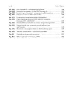
Fig. 12.1 Econometric input-output model (Panta Rhei)
Source: Meyer (1999), fig. 1, simplified; authorized copyright permission: European Communities.
environmental concerns; it ignores produced capital maintenance cost or assumes a
constant share of fixed capital consumption in GDP. GDP-based models thus assess
the potential economic cost of environmental policy, rather than the sustainability of
economic growth (cf. Section 8.3).
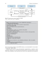
Figure 12.2 shows a decrease of CO
2
by 17% since the introduction of the eco-
tax in 1999. Since 1991, the total reduction amounts to about 25% – in line with
governmental targets at the time. The figure also presents a revised baseline scenario,
reflecting the policy situation in 2004. This scenario assumes, among others, the
introduction of EU-wide trading of capped pollution permits. As a result, Germany
should be below the year 2020 target of 800 million tons of emission, set for the
country by the Kyoto protocol.
One of the modules added in the latest version is the material flow account.
Based on export-driven demand for capital goods and diminishing effects of the
unification-caused decrease of lignite production (cf. Section 6.3.2), the model
predicts a relinkage of TMR with GDP increase. For the period 1991–2020 we
might thus see an inverted Kuznets curve, i.e. initially falling and later increasing
environmental pressure with continuing economic growth. In Factor-4 terms, the
sustainability gap shown in Figure 10.2 would be widening.
12.1 Environmental Policy Measures in General Equilibrium and Input-Output Analysis 217
218 12 Policy Analysis: Can We Make Growth Sustainable?
12.2 Environmental Constraints and Optimality:
A Linear Programming Approach
The basic input-output model does not leave anything to choice and hence to optimal,
cost minimizing or output maximizing, behaviour. As indicated (Section 12.1.1),
the introduction of pollution control cost is bound by the (shadow-priced) equality
between income and cost. Optimal behaviour is thus ‘locked’ (Dorfman et al.,
1958) in the fixed-technology model, where the equality sign of Equation (10.1)

ensures that output x is just enough to produce the given bill of final demand y.
Relaxing this built-in condition, allows production of more outputs than necessary
for predetermined y. This invites inefficiency and at the same time, opens the door
2500
2700
2900
3100
3300
3500
3700
3900
1991 1995 1999 2003 2007
Baseline
GDP
GDP
projectionn
Eco-taxed
GDP
Fig. 12.2 Panta Rhei projections of GDP and CO
2
emissions, Germany 1991–2007/2015
Source: Meyer (1999, 2005); authorized copyright permission: European Communitites.
to the possible increases of y, i.e. higher standards of living – indeed a more realistic
assumption. To stem the risk of ‘going wild’ (Chiang, 1984) with (unlimited) final
demand maximization one would have to introduce production constraints from
limited availability of primary production factors such as labour and/or environ-
mental source and sink capacities. This converts the basic input-output analysis into
optimization under constraints, i.e. into a linear programming problem [FR 12.2].
Figure 12.3 illustrates the introduction of social and environmental constraints
into the model of interdependent economic activities. Two industries of food x

1
and
shelter x
2
production face minimum requirements for food
1
and shelter
2
, and
maximum environmental limits for the emission of a pollutant
p
and the availabil-
ity of a natural resource
r
. Leaving out for now the optimizing function, these lim-
its can be expressed as constraints in a linear programming model:
()
()
1a x ax c
ax 1a x c
ax a x x
11 1 12 2 1
21 1 22 2 2
r1 1 r2 2 r
−−≥
−+− ≥
+≤ ≡ ≥xAxc- ,,
,
≤
+≤

≥
x
ax ax x
xx 0
p1 1 p2 2 p
12
(12.5)
The restrictions delimit a feasibility space (shown in highlighted boundaries in
Fig. 12.3) for different production levels and product combinations. Note that
labour is not considered a limitation in this particular model. Introducing new
environmentally sound technologies would change the pollution and resource use
coefficients, turning
p
and
r
further outward. The feasibility space would increase,
facilitating a greater scope and level of sustainable economic activity.
We can interpret the minimum requirements for food and shelter as basic human
needs of development. At the same time development is constrained by environmental
Fig. 12.3 Sustainability constraints in a linear programming model
Source: Based on Bartelmus (1979), fig. 1, p. 260; with permission by the copyright holder,
Elsevier.
12.2 Environmental Constraints and Optimality: A Linear Programming Approach 219
220 12 Policy Analysis: Can We Make Growth Sustainable?
standards. In practice, interdependent ecological, social and demographic limits are
difficult to determine. Consensus on separate limits is only a first step toward
rational targets setting as targets might overlap, for instance when determining carry-
ing capacities of human populations at different standards of living.
The practical use of a feasibility space for economic activity is therefore
questionable, especially if many more activities, outputs and standards are included.

Still, Fig. 12.3 makes the vision of sustainable development visible in terms of mini-
mum inner and maximum outer limits [FR 3.1]. At point N, basic human needs are
just met with as the lowest acceptable amounts of total outputs of food and shelter.
More importantly, the restrictions for resource availability and emissions turn the
original approach of pollution abatement (Equations 12.1) into a precautionary
model of producing within preset environmental capacity limits (cf. Section 13.2).
The introduction of an optimizing objective function turns the constrained input-output
system into a linear programming model. Figure 12.3 shows the maximum net output
(for final consumption) value Z
* for the (linear) objective function
Zvx vx
11 22
=+=
!
max
(12.6)
For given output weights of unit value added generated by the production of food
v
1
and shelter v
2
, Z* represents the highest feasible Z value. This value is indeed
another version of a maximum greened GDP (total gross value added), where
environmental and social (basic human needs) constraints are taken into account.
Introducing more than one limiting factor of production, notably produced capi-
tal, calls for considering substitution in the production functions. It also opens up
the possibility of reserving some output and natural resource reserves for future
use, i.e. capital formation and maintenance – the next section’s topic of dynamic
modelling.
12.3 Dynamic Analysis: Optimality and Sustainability

of Economic Growth
12.3.1 Dynamic Linear Programming
Section 12.2 introduced limits in the availability of scarce natural capital in a standard
linear programming model. Overuse of natural capital, i.e. either running down
natural resource stocks or degrading environmental sinks, threatens the sustainability
of economic activities. The key questions, asked repeatedly in this book, are how
close are these environmental constraints and when are we running out of environ-
mental support functions? The urgency of immediate and radical action, evoked by
environmentalists, calls for further scrutiny of the time path towards hitting potential
environmental limits. Dynamic linear programming is tailored to answering these
questions while adhering to the efficient (optimal) use – now and in the future – of
limited produced and natural capital. The challenge is to determine what amount of
produced and non-produced goods should be reserved for future use.
The basic approach of dynamic linear programming is to allow for future use of
outputs in the static system of equation 12.5. In principle, the use of outputs x
i
can
then take place either in the current period t or the future period t + 1 as
●
Inputs into different industries j during the current period: x
ij
(t), or
●
Net capital formation (including inventories of goods to be used as inputs or
final consumption in future periods), increasing the capital stock of industries by
∆= +−K K(t ) K(t)
ii i
1.
Output x
i

would now have to be large enough to cover both present and future uses:
xt x t K
iij i
() ()≥+∆
(12.7)
Further assuming fixed capital requirements b
ij
per unit of output of industry j from
industry i, and distinguishing final consumption c from capital formation ∆K
as components of final demand y, one can describe the dynamics of the two-
commodity economy as
xaxax Kc
xaxax Kc c
Kbx
1111122 11
2211222 22
111
≥++∆+
≥++∆+ ≥++
≥
xAx KD
11122
2211222
1212
bx
Kbxbx
KKxx0
+≡≥
≥+
∆∆ ≥ ≥

KBx
Kx,,, ,D 0
(12.8)
Having introduced a new primary factor, capital, the linear programming problem
is now maximizing final demand, i.e. final consumption and net capital formation,
under the restrictions of (12.8) or as its dual of minimizing capital input costs.
3
Textbooks on linear programming [FR 12.2] provide proof and explanation of the
weights attached in the objective functions of our model – either as shadow prices
of the goods and services of final demand p
i
with the objective function
∑+ =pc K
ii i
()max
!
∆
(12.9)
or as the unit shadow cost or rent r
i
of the use of the limited primary factor (capital)
k
i
with the objective function of the dual
∑=rk
ii
!
min
(12.10)
subject to prices not exceeding unit factor costs.

3
The dual of a linear programming model yields the same optimal value as the primal (in shadow
or accounting prices). The dual changes a maximization problem into a corresponding minimization
problem and vice versa. Again, we see here the income (factor cost) = net output identity described
in Section 12.1.1 for the basic Leontief model.
12.3 Dynamic Analysis: Optimality and Sustainability of Econonic Growth 221
222 12 Policy Analysis: Can We Make Growth Sustainable?
12.3.2 Optimal Growth and Sustainability
The above discussion of optimization under sustainability constraints helps
understand the introduction of environmental concerns in more generic models of
maximizing welfare and economic growth. These models are the typical, largely
theoretical, response of mainstream economists to the environmentalist critique of
ignoring long-term environmental concerns, or dealing with them at best as a matter
of short-term cost internalization. Rather than optimizing behaviour of economic
agents at the microeconomic level, optimal growth models take the view of an
overall social planner, who aims at maximizing national social welfare, now and in
the future. Welfare in turn is seen as a function of consumption of goods and
services and environmental quality. Optimal growth models thus introduce a social
welfare function, whose optimality is determined by maximizing the discounted
welfare value in each future period.
Note that in such models all time-bound variables are endogenized rather
than estimated econometrically outside the system of interdependent variables
(as in CGE models). The models go rarely beyond ‘conceptualization’ as they
abandon linearity and cling to the smooth utility and production functions of
neoclassical economics. They do succeed, though, in clearly defining long-term
sustainability of an optimizing economy – but within the particular model
assumptions [FR 12.3].
To gain insight into the meaning of highly complex multivariate dynamic opti-
mization under environmental restrictions the linear programming model can be
reformulated as a general optimization problem under an environmental constraint.

Applying the standard Lagrange multiplier method of optimization reveals the
multiplier as the shadow price (or cost) in the optimum of the linear programming
model (Dorfman et al., 1958). The multiplier thus measures the change in the value
of the objective function in a non-linear constrained optimization problem, brought
about by a marginal change in the constraint. The shadow prices of the linear
programming model can therefore be interpreted as weights for marginal changes
of final demand and capital use categories in the optimum situation (cf. Equations
12.9, 12.10).
A simplified prototype optimal growth model can elucidate these model
features. The model was initially advanced for rejecting conventional net national
product as a welfare measure due to environmental constraints (Mäler, 1991).
More recently, the model advanced a sustainability criterion, which may differ
from the optimization criterion of maximum (discounted) net present welfare. As
shown in Box 12.1, the model maximizes a social welfare function, depending on
final consumption C, capital use (including natural capital) K, environmental
damage Z, and labour input L:
WWCKZL= (,,,)
(12.11)
generated with given stocks of produced capital
1
and natural capital
2
.
The main rules and conclusions from solving the model are:
Box 12.1 Developing an optimal growth model with natural capital
STEP 1: Introducing natural capital of forests (forest inputs K
2
, logging
X, afforestation H) and sinks (pollution P and defensive expendi-
tures R) into the production function Y, with

Y = Y(K
1
, L
1
) flow of final output (aggregate production function)
X = X(K
2
, L
2
) logging rate
H = H(L
3
) net afforestation rate (incl. natural growth)
P = P(Y) pollution from producing Y
R = portion of Y devoted to mitigating pollution damage
Z = Z(R, P) net environmental damage (affecting welfare directly)
STEP 2: Specifying the model dynamics (introducing differential equa-
tions for capital formation):
dK
1
/ dt = Y(K
1
, L
1
) – C – R conventional capital formation as the difference
of final demand minus consumption C and damage mitigation R
dK
2
/ dt = H(L
3

) – X(K
2
, L
2
) net natural capital formation or depletion in
forests
STEP 3: Solving the problem of maximizing the discounted fl ow of social
welfare W over the indefi nite future. Maximizing the current
value Hamiltonian (a multivariate generalization of the Lagrange
multiplier method) obtains net social welfare along the optimal
time path as
W W C X L Z p dK dt r dK dt
12
*(,,,)(/)(/)=++
where shadow prices p and r refl ect the present value of future returns on a
marginal change in the availability of the present capital stock. W* is the sum
of current welfare W and discounted future welfare from current changes in
produced and natural capital.
Source: Dasgupta and Mäler (1991, simplifi ed).
●
Capital (incl. natural capital) maintenance rule of sustainability: if the total stock
of capital p
1
+ r
2
is valued in shadow prices along the optimal time-trajectory
of welfare generation, non-declining welfare is ensured only if the value of the
total capital stock (in constant prices) does not decrease (Mäler, 1991).
●
Intergenerational equity: the maximum Hamiltonian value, which is the

maximum welfare measure (see Box 12.1), represents the maximum feasible
consumption value that can be maintained forever. The assumptions for this
12.3 Dynamic Analysis: Optimality and Sustainability of Econonic Growth 223
224 12 Policy Analysis: Can We Make Growth Sustainable?
fortunate coincidence is that the substitution elasticity between exhaustible
natural resources and other inputs is equal or greater than 1, and that the
elasticity of the output-over-produced-capital ratio is greater than that of natural
capital (Solow, 1974a, 1974b).
●
Hartwick’s rule: for the special case of exhaustible resources, the rule requires
the reinvestment of rent (for natural capital depreciation) in reproducible capital
to ensure constant (sustainable) consumption under the above assumptions
(Hartwick, 1977).
The model outcomes thus depend, apart from the usual perfect market and substitu-
tion (in production and consumption functions) assumptions, on what is packed
into the welfare function (12.11). In particular, there is a wide variety of different,
and differently categorized, primary production factors that can be included or
ignored. Moreover, the production factors may interact in many alternative ways in
generating widely differing welfare effects. As pointed out by the authors
themselves ‘no one can seriously claim to pinpoint the optimal level of current
consumption for an actual economy’ (Arrow et al., 2004). The abstract model
serves indeed mainly the conceptualization of sustainability, specifying the need of
keeping capital intact for non-declining welfare generation.
In fact, if the welfare package is broad enough, non-decline of welfare can also
be viewed as sustainable development (Mäler, 1991). Note however that the search
for ‘empirical evidence’ for the model’s sustainability criterion had to resort to the
narrowly defined green accounting indicators of ‘genuine’ investment and wealth
(Arrow et al., 2004). These indicators are quite similar to the environmentally
adjusted capital formation (ECF) and asset indicators of the SEEA (Section 8.2.2),
catering to sustainable economic growth rather than development.

12.3.3 Some General Conclusions
Facing environmentalist adversity to economic growth, economists introduced
environmental issues in their growth models since the 1970s. As to be expected,
optimal growth analyses come to differing conclusions about the relevance
of environmental limits, depending on model assumptions. To illustrate the range
of arguments about optimality and sustainability in optimal growth models it may
suffice here to summarize the conclusions from models presented in a reader on
environmental macroeconomics (Munasinghe, 2002):
●
Technological progress can overcome resource scarcities through reduction of
extraction cost, substitution and discovery, and environmental degradation
through environmental protection. The ‘huge reserve of detailed physical,
chemical, geological and physiological relationships’ just needs to be unveiled
by ‘natural scientists and engineers’. There is no ‘clear and present case’ of a
non-substitutable resource ‘in limited supply, essential to life and welfare’
(Koopmans, 1973).
●
Technological progress, substitution of natural capital by produced capital and
increasing returns to scale make sustainable growth of per capita consumption
feasible, with optimal rates of natural resource use ‘of the order of magnitude
observed for many natural resources’ (Stiglitz, 1974).
●
With relative scarcity of natural capital and diminishing returns to technological
progress, a global steady-state economy can be reached during a transitional
period of slowing increase of labour productivity and real per capita income
growth (England, 2000).
●
Model runs show that an optimal growth trajectory and a transition to a steady-
state economy may not exist. In the absence of governmental (environmental
policy) intervention, the ecosystem collapses, and optimization and forecasting

do not produce a feasible solution. ‘An ecological economy cannot grow limit-
lessly’ (Islam, 2001).
4
Technical progress plays a crucial role in arguing the sustainability of economic
growth and its welfare effects. Most economists rely on human knowledge and
inventiveness as the saviour from environmental and related economic collapse.
Environmentalists, on the other hand, point to the physical laws of entropy and
complementarity in the use of energy and materials: critical natural capital is bound
to run out eventually if current demographic and economic growth patterns
continue. Empirical evidence seems to be on the side of the economists, at least as
far as natural resource depletion is concerned. Decreasing natural resource prices
indicate reduced scarcity for many natural resources. As a result, we could expect
an increase in ‘effective’ natural resource stocks.
5
But all depends, of course, on our
ingenuity. Will technology be the saviour? Possibly.
Parts II and III assessed empirically the impacts and repercussions of the
environment-economy interaction. In this part we used these assessments, at least
in principle, for prediction and policy analysis. However, simplifying model
assumptions and selectivity in model variables usually impair practical policy
advice. On the other hand, introducing the value-laden vision of sustainable
development into economic theory gives us a more rigorous understanding of the
paradigm. The result is a pragmatic focus on the sustainability of economic growth
in applied and theoretical environmental-economic analyses. The final part of the
book makes use of our visionary, empirical and analytical knowledge to offer a few
strategic ‘conclusions’. Admittedly, these conclusions are far from conclusive, as
indicated by a final chapter on remaining ‘questions’.
4
One should probably not read too much into the progressive greening of the economists, as time
goes by.

5
Barnett and Morse are among the first to find a long-term decrease in real extraction cost of most
minerals. See also the Simon-Ehrlich wager [FR. 11.2]. According to Baumol (1986), ‘effective
natural resource stock’ (even of non-renewable resources) might increase when technological
innovation leads to a revision of usable resource stocks at a rate that exceeds resource use.
12.3 Dynamic Analysis: Optimality and Sustainability of Econonic Growth 225
226 12 Policy Analysis: Can We Make Growth Sustainable?
Further Reading
FR 12.1 Computable General Equilibrium
Munasinghe’s (2002) reader on Macroeconomics and the Environment gives an
overview of environmental-economic analysis and modelling. Computable general
equilibrium (CGE) models play a prominent role in this review. Conrad (1999)
provides a concise description of the ‘principles’ of CGE models of environmental-
economic policy analyses. Most applied CGE models are based on input-output
tables and analysis [FR 10.1] for determining their benchmark situation.
Quite unusual for a statistical office, Statistics Norway seems to have moved from
descriptive natural resource accounting to introducing environmental concerns and
energy consumption into a multi-sectoral dynamic CGE model ( />emner/09/90/rapp_200418/rapp_200418.pdf; Alfsen, 1996). A dynamic CGE model
of the USA compares a backcasted scenario without environmental regulation with
the actual regulated situation: for 1973–1985 GDP has been reduced by 2.59%
owing to environmental protection (Jorgenson & Wilcoxen, 1990).
As part of an EU investigation into green accounting the GREENSTAMP project
suggests to replace the green GDP by a modelled ‘greened’ GDP, i.e. ‘a hypothetical
national economic product that would be obtainable … subject to … a specified set of
environmental standards’ (O’Connor, 1999). Model results indicate that the combina-
tion of technology and ‘sustainable consumption’ allows standards of living in France
to improve while respecting sustainability standards. The model restricts, however, its
environmental policy analysis to energy consumption and its pollution effects.
FR 12.2 Linear Programming and Economic Analysis
Dorfman et al. (1958) is probably still the best text on the use of linear program-

ming in economic analysis. Much of Sections 12.2 and 12.3.1 is based on this book.
Paris (1991) focuses on duality in economic applications of linear programming
such as factor cost minimization for given final demand as the dual of GDP maximization
with given primary factors (cf. Section 12.2). Textbooks on economic mathematics
(such as Chiang, 1984) may facilitate access to the sometimes-challenging
mathematics of linear and non-linear, and dynamic programming. An early call for
applying linear programming or activity analysis to the assessment of sustainability
limits in ‘eco-development’ (Bartelmus, 1979) went largely unheeded.
FR 12.3 Sustainability in Optimal Growth Models
Mainstream economists extended optimal growth models of inter-temporal welfare
maximization to natural capital endowment. Some of these models, whose main
findings are cited in the text, can be found in Munasinghe (2002). Dasgupta and
Mäler (1991, 2000) use the model to delineate an environmentally modified net
national product indicator as a welfare measure that reflects optimal growth as well
as sustainability. Arrow et al. (2004) explain that the maximum welfare value of
this model does note have to coincide with sustainability in the sense of perpetual
constant per capita consumption. Pointing out this discrepancy may be the reason
for co-opting environmentalists like Paul Ehrlich and Gretchen Daily as co-authors
of this article. It remains to be seen if some euphoria about the ‘friendship’ between
environmentalists and economists (Christensen, 2005) will stand the test of time,
especially when environmentalists obtain a clearer picture of the model
assumptions.
Review and Exploration
●
Explain the differences and relationships between input-output and CGE
models. How do they deal with environmental impacts and policies?
●
Is a ‘greened’ (modelled) GDP preferable to a green (accounted) GDP/NDP for
supporting sustainability in policymaking? Compare the different greened GDPs
resulting from CGE, linear programming and optimal growth models.

●
What is the purpose of dynamic modelling? How does it compare to comparative-
static (CGE) analysis? Can it capture the (non)sustainability of economic
growth?
●
What are your conclusions about the use and usefulness of modelling – vs. direct
data use – for policymaking?
●
Is technology the saviour from environmental collapse?
Review and Exploration 227
Part V
Strategic Outlook
Part IV’s analysis of potential limits to economic growth at national and global
levels sets the tone for some strategic conclusions about tackling these limits.
Chapter 13 presents strategies and policy measures for dealing with impacts of
production and consumption that threaten to violate environmental limits. The
strategies apply mostly to governmental policy but include also voluntary action by
corporations and households, motivated by a new environmental ethics. Global and
trans-boundary environmental impacts require international action. Chapter 14
examines, therefore, the need for improving global governance in order to advance
sustainable growth and development in a globalizing world.
The concluding chapter raises again the initial questions of Part I and asks what
we learned about them. Many conclusions remain tentative and raise further ques-
tions. It is thus quite appropriate to end the book as it began with a chapter on
‘questions, questions, questions’. This should not be taken as resignation before a
host of open issues, but rather as encouragement of further quantitative analyses.
Chapter 13
Tackling the Limits to Growth
None of the above-described indicators and models provides an unequivocal
answer to whether economic growth, and what kind of growth, are sustainable.

Rather, the dichotomy between pessimistic environmentalists and more optimistic
economists persists in measurement and analysis of the environment-economy
interaction. So what should and could be done about an undeniable problem, whose
significance is judged differently?
To be on the safe side let us set out from the pessimistic view of the Limits-to-
Growth (LTG) model. The model explains environmental impacts in terms of the
popular IPAT identity as the result of population growth, wasteful affluence, and
effects of the energy needs of technology (Meadows et al., 2004).
1
The model’s
more optimistic, but ‘less likely’ scenarios reveal ‘responses’ to non-sustainable
resource depletion and pollution, which together would attain sustainable develop-
ment (op. cit.; see also Section 11.2.1):
●
Population control by means of birth control, which should limit reproduction
to two children per family (scenario 7)
●
Plus: limiting industrial output by means of moderation in lifestyles and more
efficient capital use, in other words greater sufficiency in consumption and
greater eco-efficiency in production (scenario 8)
●
Plus: technological progress in reducing the remaining pollution (scenario 9).
Birth control and sufficiency are the results of changes in individual behaviour. On
the other hand, deliberate R&D or spontaneous inventions of creative minds bring
about environmental technologies. For generating these behavioural and techno-
logical changes the LTG authors leave their mechanistic model and call for ‘leader-
ship and ethics, vision and courage’, supported by a ‘networking’ civil society.
As hard-nosed economists we want to go beyond ‘heart-felt intuition’ (op. cit.)
about changes in social values and enlightened leadership. This is not to deny the
importance of ethics and ‘soft’ strategies of moral suasion (Section 13.4). However,

1
I = PAT defines impacts I as the result of three determinants: (1) size of population P, (2) affluence
A as GDP p.c. and (3) technology as ‘eco-efficiency’ I/GDP. This reveals IPAT as an identity:
I = P × GDP/P × I/GDP ≡ I.
P. Bartelmus, Quantitative Eco-nomics, 231
© Springer Science + Business Media B.V. 2008
232 13 Tackling the Limits to Growth
the objective of this book is to facilitate and evaluate rational policies with the quan-
titative measures and analyses described in the preceding parts. It would fill another
book to detail the effects of different economic, social and environmental policies on
economic growth and development. The way to confine the discussion of policy
measures, besides leaving much to further reading, is to bundle these measures under
four basic strategies of dealing with potential environmental limits:
●
Ignoring the limits: muddling through
●
Complying with limits: curbing economic activity
●
Pushing the limits: improving eco-efficiency
●
Adopting limits: sufficiency in consumption, corporate social responsibility,
environmental ethics.
13.1 Ignoring the Limits: Muddling Through
Tackling environmental symptoms when they occur and relying on past experience
for taking action can be seen as a muddling-through policy. One view considers
such ad hoc reaction as more realistic than comprehensive (costly and time con-
suming) analyses of fundamental objectives and policy options (Lindblom, 1959).
If past experience includes reliance on market forces for signalling a problem and
adjusting to its effects, we have a particular form of muddling through. The stalwart
of market liberalism, The Economist (of 11 September 1999) argues that experi-

mentation by markets is ‘a humbler way of going about things than by following
the conceited blueprints of politicians, the hubris of monopolistic businessmen, or
the arrogance of scientists’; history shows that governments and pressure groups
frequently impose their visions – only to abandon them later as mistaken.
As discussed in Section 11.1, the EKC hypothesis is an attempt to justify non-
interference in market activities. The assumption is that unfettered economic per-
formance and growth solve environmental problems automatically, or at least
facilitate their solution. However, our review of the hypothesis did not find conclu-
sive evidence for a general correlation between economic growth and environmental
improvement in the high-income range of the EKC. The dominant force behind
environmental improvement appears indeed to be environmental policy, frequently
marginalized, however, even in rich countries. It is thus an open question, whether
such policy is driven by affluence or by necessity (cf. Section 11.1.2).
Relying on economic growth alone does not seem to be a valid option. On the
other hand, there is some evidence that the price signals of the market do reflect
natural resource scarcity as in the case of falling prices of mineral commodities
(Section 12.3.3). By the same token, rising prices would indicate increasing scar-
city and might stimulate the search for more efficient extraction, harvesting and use
of natural resources. Adaptation of car use at the peak of gasoline prices is a case
in point. The question is whether such observations can be generalized. Short-sighted
non-action looks indeed suspiciously like ‘passing the buck to future generations
and other regions’ (Rothman, 1998).
Again, we see here the environmentalist-economist dichotomy at work when
dealing with uncertainty or ignorance about environmental damage. Environmental
economists take a wait-and-see attitude. They look first for market signals of new
scarcities in environmental source and sink services before internalizing the scar-
city costs. They also discount uncertain environmental risks according to their
preference for current vs. future benefits and, inversely, cost (cf. Section 2.3.2).
Ecological economists, on the other hand, call for urgent precautionary and regula-
tory action, in the face of imminent disaster.

13.2 Complying with Limits: Curbing Economic Activity
Facing up to environmental disaster most environmentalists show hostility toward
economic growth, albeit with some focus on the physical side of economic expan-
sion. Their idea of sustainable development can be characterized as ‘development
without growth – without growth in throughput beyond environmental regenerative
and absorptive capacities’ (Daly, 1996). This would indeed leave the door open to
economic growth (expressed in real, constant-price values) as long as it does not
violate environmental carrying capacities. For the limitation of the physical scale
of economic activity, the use of popular environmental ‘management rules’ is the
prevailing policy advice (Daly, 1990; Sachs et al., 1998):
●
Use renewable resources within their regenerative capacity.
●
Use non-renewable resources as far as renewable substitutes can be found.
●
Discharge waste and residuals without exceeding the absorptive capacities of
natural systems.
For concrete policy measures, these rules require specific targets or (safe minimum)
standards of natural resource use and emissions and their ambient concentrations.
Setting ecological standards at the national (policy) level is problematic but could
delimit economic activities within a normative feasibility space (Sections 3.2.2 and
12.2). From the point of view of an already overloaded full-world economy, regula-
tory command and control (CAC) of economic activity is the preferred policy
instrument for forcing economic activity into the feasibility space. CAC rules and
regulations aim at directly reducing the scale of throughput and corresponding eco-
nomic activity as the prime ecological sustainability objective.
However, economic activity can be curbed not only by regulating material flows to
and from the economy but also by market instruments. Seeking an optimal level of –
monetary – output through environmental costing, output is usually lower than the one
generated by unfettered markets (cf. Annex I for the case of a Pigovian eco-tax). It

might be higher, though, than the level brought about by CAC, owing to the economic
and technological prowess of enterprises in reducing environmental impacts and costs.
Both approaches could be combined: CAC measures could set and enforce the feasibil-
ity space, and the market could then determine efficient – after environmental cost
internalization – production and consumption patterns within this space.
13.2 Complying with Limits: Curbing Economic Activity 233
234 13 Tackling the Limits to Growth
Table 13.1 presents a taxonomy of typically applied environmental policy measures.
CAC specify what (which policy target) needs to be achieved and how it should be
achieved, e.g. by prohibiting the use of specific inputs, prescribing particular tech-
nologies, or protecting the use of land from economic development. A popular
way of creating protected areas in developing countries, are debt-for-nature swaps.
The idea is to grant foreign debt relief in exchange for abstaining from economic
land use.
2
The other parts of the table indicate various possibilities of relaxing either
the setting of targets or prescribing the way of target implementation, or both, for
applying more flexible market instruments (see also Annex I.2).
The reason for using the drastic CAC measures is, besides their simplicity of
application, lack of trust in the capability of market forces to reach society’s
environmental goals. Doubt in market solutions stems from
Table 13.1 Taxonomy of environmental policy instruments
Policy target specified Policy target not specified
‘How’ specified
(implementation
process
prescribed)
CAC:
- Prohibitions (of hazardous inputs,
discharges and overuse of natural

resources)
- Environmental standards and
technology specified (incl. recy-
cling/reuse)
- Land appropriation, purchase or
expropriation for environmental
protection
- Obligatory insurance for specific
environmental impacts
- Subsidies for particular equipment
- Transfer of technology
- Liability (with care standard)
‘How’ not specified
(implementation
process not
prescribed)
- Tradable pollution and resource
use permits (cap and trade)
- Design and performance standards
- Voluntary agreements (including
environmental audits, labelling
etc.)
- Emission and product charges
- Resource rent capture (royalties)
- Deposit-refund system
- Technical assistance (open-ended)
- Property rights for environmental
sinks and sources (bargaining)
- Liability (without care standard)
- Subsidies (open-ended, grants and

removal of subsidies)
- Environmental information and
education
Source: Russel. Clifford S. (2001), Applying economics to the environment, table 9.3, modified;
with permission by the copyright holder, Oxford University Press.
2
Preventing economic development for the creation of nature reserves meets of course with the
resistance of land owners or users facing governmental land appropriation. Typically, international
NGOs such as the WWF ( initiate
these swaps with some financial contribution; ultimately the swaps require a formal agreement
between the creditor and debtor country.
●
A tendency of economic agents to underestimate uncertain potential environ-
mental damage
●
Possible ‘irreversibilities’ of environmental damage, for which time-lagged indi-
vidual responses to market incentives might come too late.
Immediate and fully controlled environmental action makes sense for averting
imminent environmental disaster. The precautionary principle of the Rio Declaration
(United Nations, 1994, Rio Declaration, Principle 15) points in that direction in a
less stringent manner: ‘lack of full scientific certainty shall not be used as a reason
for postponing cost-effective measures to prevent environmental degradation’.
A simpler popular formulation is to be better approximately right in time than
optimally right too late.
It comes as no surprise that ecological economists adopted this principle as a
justification for preferring proactive rules and regulations to reactive market instru-
ments (cf. Section 2.4). The question is, whether governments are indeed in a better
position – than individual preferences expressed in markets – to weigh uncertain
risks against the cost of reducing the risks.
3

In fact there is no good reason why the
above-mentioned management rules could not be relaxed in some cases. Why should
we forgo decreasing some of the natural resource stocks, e.g. for current poverty
alleviation, when future requirements for the resources are highly uncertain?
13.3 Pushing the Limits: Eco-Efficiency
Typically the political process, rather than rational quantitative analysis, guides
CAC action. CAC is thus particularly inefficient when economic agents possess
better information than remote and sluggish bureaucracies. The objective of market
instruments of environmental policy is to prompt consumers and producers into
using this information under competitive pressure. Eco-efficient production and
consumption patterns are the expected results.
13.3.1 Eco-Efficiency and Resource Productivity
CAC prescription of existing technologies thwarts human ingenuity in finding innovative
and least-cost solutions to environmental problems. This is the reason for letting
market forces search for ecologically and economically efficient products and pro-
duction processes. The World Business Council for Sustainable Development
defines such ‘eco-efficiency’ as ‘a management strategy [of corporations] that links
financial and environmental performance to create more value with less ecological
3
A survey by The Economist (of January 2004) presented several examples of conspicuous failures
of governments to reasonably balance risks and net returns from protection against risk, notably in
the areas of hazardous pollution, BSE (mad cow disease) and the US fight against terrorism.
13.3 Pushing the Limits: Eco-Efficiency 235
236 13 Tackling the Limits to Growth
impact’ [FR 13.1]. Environmental economists also favour the supply side of market
exchange, considering consumers hardly knowledgeable about production and
emission processes (Turner et al., 1993). Economic modelling confirms that new
environmentally sound technologies can open up the feasibility space for economic
activity by pushing outward environmental source and sink limits (cf. Fig. 12.3).
Faith in eco-efficient technology is most pronounced in the concept of metabolic

consistency [FR 13.1]. The idea is to imitate nature, which ‘does not know the con-
cept of waste’.
4
One of the protagonists of consistency sees the seamless incorpora-
tion of industrial metabolism into nature’s metabolism as a paradigm shift from
quantitative eco-efficiency to new qualitative innovation (Huber, 2004). The purpose
is still to maximize production and minimize environmental impact. A more modest
view of consistency might see it, therefore, as a particularly efficient type of eco-
efficiency. Plate 13.1 is a simplified example of how waste from coffee production
can be channelled into a highly profitable side activity – mushroom breeding. In fact,
in this case study, revenues from sales of shitake exceeded those of coffee.
Eco-efficiency has also become the basic tenets of industrial ecology, a rela-
tively new field of research on industrial metabolism, i.e. material flow analysis at
the enterprise level (Lifset & Graedel, 2002). Sections 2.4.2 and 6.3.1 presented
resource productivity (GDP per material input) as the key indicator of ecological
sustainability at the macroeconomic level. The connection between micro-level
corporate eco-efficiency and macro-level national or regional resource productivity
is not straightforward, however. There appears to be some wishful thinking about
corporate social responsibility (CSR), which would motivate enterprises to reduce
natural resource use and emissions for the sake of the greater social good. In prac-
tice, neither corporate environmental accounting nor environmental management
are likely to fully embrace any goals beyond cost saving and corporate image
improvement (Sections 9.1.1 and 9.2).
Eco-efficiency remains thus most useful as a macroeconomic objective for
policy instruments that influence the behaviour of microeconomic agents. To this
end, eco-efficiency and its instruments address both sides of the material flow
balance with the objectives of
●
Increasing resource productivity (GDP/DMI) for the dematerialization of the
economy

●
Decreasing environmental impact intensity (DPO/GDP) or its inverse, pollution
‘efficiency’ (GDP/DPO) for the detoxification of the economy.
5
4
According to the ‘vision’ of the Zero Emissions Research Initiative (ZERI) ( />index.cfm?id = vision). Considering the ‘waste’ of large amounts of seeds that do not germinate,
Ehrenfeld and Chertow (2002) contest this view and prefer referring to ‘nature’s bounty … as
eco-effectiveness’.
5
See Section 6.3.1 for the definitions of the material flow indicators. As also discussed in that
section, detoxification can either be considered as a supplementary sustainability concept or sub-
sumed under the general notion of dematerialization.
The EU strategy on the sustainable use of natural resources (Commission of the
European Communities, 2005, annex 3) defines eco-efficiency (EE) as the ratio of
resource productivity (value added per material input: VA/MI) and ‘resource spe-
cific [pollution] impact’ (I/MI):
EE VA/MI: I/MI VA/I==
(13.1)
Environmental impact, i.e. the generation of residuals over the life cycle of a product,
results from direct and indirect (‘upstream’) material inputs. Eco-efficiency seems
thus to be reduced to value added per unit of wastes and residuals, ignoring the
potential depletion of natural resources used. This is probably an unintended result
of the EU’s eco-efficiency definition since the strategy calls for the simultaneous
reduction of environmental impacts and the improvement of resource productivity.
At any rate, reference to the product life cycle introduces indeterminate time periods
Plate 13.1 Metabolic consistency: coffee and mushroom production
Source: Based on Steinbrink (2001), fi g. 2; with permission by the copyright holder, Zero Emission
Research Initiative, ZERI (See Colour Plates).
13.3 Pushing the Limits: Eco-Efficiency 237
238 13 Tackling the Limits to Growth

into microeconomic impact assessment, complicating annual national-accounts-
based macro-analysis of eco-efficiency.
The EU strategy remains thus just this: a strategy that seeks to achieve
dematerialization but lacks an operational concept for implementation. The
strategy refrains, therefore, from adopting the targets of the EU’s Sixth
Environment Action Programme due to lack of knowledge and indicators. As
discussed in Section 2.4.2, determining the amount of dematerialization needed
for sustainability requires the setting of national targets, or at least guardrails,
such as Factor 4 or 10. For structural and regional policies, one would also have
to specify compatible standards at regional and sectoral levels. A variety of
policy instruments, including the above-described CAC measures and market-
based ‘economic instruments’ can be applied for meeting eco-efficiency targets
and standards.
13.3.2 Categories and Efficiency of Market Instruments
13.3.2.1 Strategic Principles
Market instruments can improve both ecological and economic sustainability [FR
13.2]. Ecological sustainability would use these instruments for reducing material
input and residual output by increasing the cost of material inputs and penalizing
wastes and emissions. Stressing, however, the inability of markets to achieve
distributive equity or sustainable scale, ecological economists rank the allocative
efficiency of market instruments lower than setting scale and equity limits (Daly &
Farley, 2004; Costanza et al., 1997a).
Economic sustainability aims at the internalization and eventual reduction of
environmental cost according to the polluter/user-pays principles (PPP, UPP).
Contrary to the precautionary principle, which caters to a preventative CAC
approach, the PPP and UPP seek to burden those who caused pollution, congestion
and natural resource depletion with the cost of damage mitigation or compensation.
To the extent that cost anticipation deters economic agents from polluting or
depleting, the two principles may also have precautionary effects. The UPP is less
clearly defined. It refers usually to natural resource use by corporations but could

also include the responsibility of consumers for their wasteful consumption of
environmentally damaging products.
Initial environmental cost internalization and full-cost pricing by enterprises
does not mean that producers have to bear all the cost. Depending on price
elasticities of supply and demand, enterprises might be able to share the effects of
cost-pushed price increase with consumers. At the international level, shared
responsibility for outsourcing hazardous production processes and importing
natural resources would justify some compensation of sustainability ‘exporting’
countries by the importers (cf. Section 6.3.2).
A more specific microeconomic formulation of the UPP focuses on the compensation
of providers or protectors of ecological services. The International Union for
Conservation of Nature and Natural Resources (IUCN) has been promoting
eco-compensation according to the benefits of ecological services provided, or the
– damage – cost of their loss. Considering such benefit or damage as externalities
of economic activity, their internalization in the budgets of households and enter-
prises would be desirable from optimal production and consumption points of view.
The drawbacks are measurement and valuation problems of ecosystem services
(Sections 2.4.1, 8.1.3). On the other hand, case studies indicate that in particular
situations, the carrot of subsidies and the pacifier of compensation (e.g. for giving
up land development for eco-system maintenance) may be conducive to ‘harmonious’
development
6
[FR 13.2].
13.3.2.2 Market (Dis)incentives
Different market instruments show different economic and ecological effectiveness.
A brief evaluation of the main categories of these instruments gives a first impres-
sion of their use, usefulness and information requirements for setting them at an
‘appropriate’ level. As discussed in Section 2.3.2 and Annex I, one would ideally
seek to set the incentive for environmental cost internalization at the optimal level.
At that level, the sum of marginal environmental damage and conventional eco-

nomic cost equals marginal revenue. In practice, some kind of heuristic standard
costing, as applied in green accounting, is probably the only way for an informed
setting of market instruments.
Table 13.1 distinguishes market instruments from ‘hard’ CAC measures by
relaxing the prescription of what environmental protection should achieve and/
or how environmental measures should be carried out. ‘Soft’ instruments of
education, information, environmental subsidies and voluntary agreements are
most ‘relaxed’ as their application is usually optional. More incisive tools,
which set clear standards and disincentives to prevent or reduce the violation of
environmental standards, can be categorized as ‘semi-soft’ (or semi-hard). They
are the most promising tools in changing the environmental behaviour of
producers and consumers.
Table 13.2 evaluates common environmental policy instruments as to their
ecological and economic efficiency and practicality. Market instruments either create
new markets, or attempt to influence market behaviour by incentives for environ-
mentally friendly and disincentives for environmentally damaging production and
consumption. Actual applications frequently combine different instruments of
incentive subsidies and disincentive charges and taxes. Pigovian eco-taxes, deposit-
6
Harmonious development is the fundamental principle of tackling the social impacts of acceler-
ated economic growth in China (Li et al., 2007).
13.3 Pushing the Limits: Eco-Efficiency 239
240 13 Tackling the Limits to Growth
Table 13.2 Evaluation of environmental policy instruments
+−
Command and control
(hard instruments)
- Prohibition
- Standards and
regulations

- High and rapid efficiency
(in case of uncertainty about
impacts)
- Effective monitoring and
control
- Most incisive for high-risk
impacts (precautionary prin-
ciple)
- Recycling/reuse applications
- Transparency facilitates
acceptance
- Economic inefficiency (in
finding least-cost solutions)
- ‘Freezing’ existing (best avail-
able) technology
- Delays in application from
legislative process
Market disincentives
- Charges/taxes on emis-
sions, products and natu-
ral resource use
- Removal of environmen-
tally damaging subsidies
- Deposit-refund systems
(recycling)
- Economic and ecological effi-
ciency
- Prompting innovation
- Generation of revenue
- Fiscal neutrality of eco-tax

reform
- Politically set levels of disin-
centive
- Sectoral rather than microeco-
nomic application
- Implementation delays
- Limited acceptance
- Limited coverage of pollutants
- High cost incidence with
inelastic demand
- Difficult (‘optimal’) damage
estimation and valuation
- Regressive taxation
Market creation
- Property rights and
bargaining
- Tradable permits
- Greater care for owned assets
- Property rights for sink functions
- Cap-and-trade paradigm (com-
bining standards and market
forces/preferences)
- Application at national and
international levels
- Transaction cost of bargaining
(identification of agents and
impacts)
- Imperfect markets
- Political standard setting
- Limited coverage of pollutants

- Ignoring local effects
- Imperfect markets
Soft instruments
- Subsidies
- Education
- Information
- Voluntary agreements
- Changing consumption
patterns
- Non-economic sustainability
concerns (equity, ethics)
- Acceptance of policy measures
- Supporting innovation
- Low implementation cost
- Limited adherence to volun-
tary agreements
- Negative economic and eco-
logical effects of subsidies
- Advocacy by interest groups
(moral suasion)
refund systems and tradable pollution permits are the most commonly used instruments.
After its success in London, congestion pricing is being considered in many other
cities for reducing rush hour traffic and pollution. Daly (1996) even considers
cap-and-trade policies, extended beyond emission trading to natural resource use,
as a ‘paradigm’ for ecological economics: the initial capping caters to the primary
goal of ecological sustainability as a ‘scale limit’ while trading of environmental
credits allows for allocative efficiency of conventional economics.