Quantitative Techniques for Competition and Antitrust Analysis by Peter Davis and Eliana Garcés_8 pptx

268 5. The Relationship between Market Structure and Price
S
N
1
2
S
1
S
2
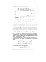
Figure 5.6. The concave relationship between number of
firms and market size from a Cournot model.
And in a symmetric equilibrium we can describe equilibrium prices and quantities,
respectively, as
p

i
D
a
b

1
b
Nq

i
S
and q

i
D
S.a  bc/

N C 1
:
As in the previous section, we substitute the optimal quantity back into the profit
equation:
˘
i
D p

i
q

i
 cq

i
 F
D
Â
a
b

N
bS
Â
S.a  bc/
N C 1
Ã
 c
ÃÂ
S.a  bc/

N C 1
Ã
 F
D
Â
a  bc
N C 1
Ã
2
S
b
 F:
For the firm to break even, we need at least ˘
i
D 0. If we solve for the corresponding
equilibrium number of firms, we obtain
N

D .a  bc/
r
S
bF
 1:
The number of firms is therefore concave in market size S.
The Cournot equilibrium derived above is somewhat special in that, to make the
algebra simple, we assumed constant marginal costs. Constant marginal costs are
the result of constant returns to scale and, as we noted previously, such a technology
effectively imposes no constraint on the scale of the firm. An alternative assumption
would be to introduce convex costs, i.e., we could assume that at least eventually
decreasing returns to scale set in. In that case, while we will still obtain the same

result of concavity for smaller market sizes, we will find that as market size increases
5.2. Entry, Exit, and Pricing Power 269
the relationship becomes approximately linear. Such a feature emphasizes that in the
limit, asmarket size getsbig, the Cournotmodel becomes approximatelycompetitive
and close to the case described for the price-taking firms with decreasing returns.
With a large number of firms, the effect of the diseconomies of scale sets in and the
size of an individual firm is then mainly determined by technological factors while
the number of active firms is determined by the size of the market.
5.2.3 Entry and Market Power
The previous sections explained the basic elements of the entry game and described
particularly how market size, demand, technology, and the nature of competitive
interaction will determine expected profitability and this in turn will determine the
observed number of firms. An interesting consequence of these results is that they
suggest we can potentially learn about the intensity of competition by observing how
entry decisions occur. Bresnahan and Reiss (1990, 1991a,b) show that for this class
of models, if we establish the minimum market size required for the incumbents to
operate and the minimum market size for a competitor to enter, we can potentially
infer the market power of the incumbents. In other words, we can potentially use
the observed relationship between the number of firms and the size of the market
to learn about the profitability of firms. Specifically, we can potentially retrieve
information on markups or the importance of fixed costs. Consequently, we can
learn about the extent to which margins and market power erodes as entry occurs
and markets increase in size.
5.2.3.1 Market Power and Entry Thresholds
In this section, we examine the change in the minimum market size needed for the
N th firm s
N
as N grows. Particularly, we are interested in the ratio of the minimum
market size an entrant needs to the minimum market size the previous firm needed to
enter, s

N C1
=s
N
. If entrants face the same fixed and variable costs than incumbents
and entry does not change the nature of competition, then the ratio of minimum
market sizes a firm needs for profitability is equal to 1. This means the .N C 1/th
firm needs the same scale of operation as the N th firm to be profitable. If on the
other hand entry increases competitiveness and decreases margins, then the ratio
s
N C1
=s
N
will be bigger than 1 and will tend to 1 as N increases and margins
converge downward to their competitive levels. If fixed or marginal costs are higher
for the entrant, then the market size necessary for entry will be even higher for the
new entrant. If s
N C1
=s
N
is above 1 and decreasing in N , we can deduce that entry
progressively decreases market power.
Given the minimum size s
N
required for entry introduced above
s
N
D
S
N
D

F
ŒP
N
 AV C d.P
N
/
:
270 5. The Relationship between Market Structure and Price
We have
s
N C1
s
N
D
F
N C1
F
N
ŒP
N
 AV C
N
d.P
N
/
ŒP
N C1
 AV C
N C1
d.P

N C1
/
:
If marginal and fixed costs are constant across entrants, then the relation simplifies
to
s
N C1
s
N
D
ŒP
N
 cd.P
N
/
ŒP
N C1
 cd.P
N C1
/
so that the ratio describes precisely the evolution in relative margins per customer.
5.2.3.2 Empirical Estimation of Entry Thresholds
Bresnahan and Reiss (1990, 1991a,b) provide a methodology for estimating succes-
sive entry thresholds in an industry using data from a cross-section of local markets.
In principle, we could retrieve successive market size thresholds for entry by observ-
ing the profitability of firms as the number of competing firms increases. However,
profitability is often difficult to observe. Nonetheless, by using data on the observed
number of entrants at different market sizes from a cross section of markets we may
learn about the relationship.
First, Bresnahan and Reiss specify a reduced-form profit function which repre-

sents the net present value of the benefits of entering the market when there are N
active firms. The reduced form can be motivated by plugging in the profit function
the equilibrium quantities and prices obtained from an equilibrium to a second-stage
competitive interaction between a set of N active firms, following the game outlined
in figure 5.1, and, say, the price-taking or Cournot examples presented above. The
profit available to a firm if N firms decide to enter the market can then be expressed
as a function of structural parameters and be modeled as
˘
N
.X;Y;WIÂ
1
/ D V
N
.XI˛; ˇ/S.Y I/  F
N
.W I/ C " D
N
˘
N
C ";
where X are the variables that shift individual demand and variable costs, W are
variables that shift fixed costs, and Y are variables that affect the size of the market.
The error term " captures the component of realized profits that is determined by
other unobserved market-specific factors. If we follow Bresnahan and Reiss directly,
then we would assume that the "s are normal and i.i.d. across markets, so that
profitability of successive entrants is only expected to vary because of changes in
the observed variables. Note that this formulation assumes that firms are identical
and is primarily appropriate for analyzing market-level data sets. A generalization
which is appropriate for firm-level data and also allows firms to be heterogeneous
in profitability at the entry stage of this game is provided by Berry (1992).

Bresnahan and Reiss apply their method to several data sets each of which doc-
uments both estimates of market size and the number of firms in a cross section
of small local markets. Examples include plumbers and dentists. To ensure inde-
pendence across markets, they restrict their analysis to markets which are distinct
5.2. Entry, Exit, and Pricing Power 271
geographically and for which data on the potential determinants of market size can
be collected. The variables explaining potential market size, Y
m
, include the pop-
ulation of a market area, the nearby population, population growth, and number
of commuters. The variable used to predict fixed costs for the activities that they
consider is the price of land, W
m
. Variables included in X
m
are those affecting the
per customer profitability. For example, the per capita income and factors affecting
marginal costs. The specification allows variable and fixed costs to vary with the
number of firms in the market so that later entrants may be more efficient or require
higher fixed costs.
Denoting market m D 1;:::;M we may parameterize the model by assuming
S.Y
m
I/ D 
0
Y
m
;
V
N

D X
0
m
ˇ C˛
1

Â
N
X
nD2
˛
n
Ã
;
F
N
D W
m

L
C 
1
C
N
X
nD2

n
:
In order to identify a constant in the variable profit function, at least one element of

 must be normalized, so we set 
1
D 1. Note that changes in the intercept, which
arise from the gammas in the fixed cost equation, capture the changes in the level
of profitability that may occur for successive entrants while changes in the alphas
affect the profitability per potential customer in the market. The alphas capture the
idea, in particular, that margins may fall as the number of firms increases. Note that
all the variables in this model are market-level variables so there is no firm-level
heterogeneity in the model. This has the advantage of making the model very simple
to estimate and requiring little in the way of data. (And we have already mentioned
the generalization to allow for firm heterogeneity provided by Berry (1994).) The
parametric model to be estimated is
˘
N
.X
m
;Y
m
;W
m
;"
m
IÂ
1
/
D
N
˘
N
C "

m
D V
N
.X
m
I˛; ˇ/S.Y
m
I/  F
N
.W
m
I/ C "
m
D
Â
X
0
m
ˇ C˛
1

N
m
X
nD2
˛
n
Ã
.
0

Y
m
/  W
m

L
 
1

N
m
X
nD2

n
C "
m
;
where "
m
is a market-level unobservable incorporated into the model. A market will
have N firms operating in equilibrium if the N th firm to enter is making profits but
the .N C 1/th firm would not find entry profitable. Formally, we will observe N
firms in a market if
˘
N
.X
m
;Y
m

;W
m
IÂ
1
/ > 0 and ˘
N C1
.X
m
;Y
m
;W
m
IÂ
1
/<0:
272 5. The Relationship between Market Structure and Price
−
N+1
Π
−
N
Π
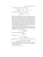
Figure 5.7. The cumulative distribution function F ."/ and the part of
the distribution for which exactly N firms will enter the market.
Given an assumed distribution for "
m
, the probability of fulfilling this condition for
any value of N can be calculated:
P.˘
N

.Y;W;ZIÂ
1
/ > 0 and ˘
N C1
.Y;W;ZIÂ
1
/<0j Y; W; ZIÂ
1
/
H)
P.
N
˘
N
.Y;W;ZIÂ
1
/ C " > 0 and
N
˘
N C1
.Y;W;ZIÂ
1
/ C "<0j Y; W; ZIÂ
1
/
D P.
N
˘
N
.Y;W;ZIÂ

1
/ 6 "<
N
˘
N C1
.Y;W;ZIÂ
1
/ j Y; W; ZIÂ
1
/
D F
"
.
N
˘
N C1
IÂ
1
/  F
"
.
N
˘
N
IÂ
1
/;
where the final equality follows provided the market-specific profitability shock "
m
is conditionally independent of our market-level data .Y

m
;W
m
;Z
m
/. Such a model
can be estimated using standard ordered discrete choice models such as the ordered
logit or ordered probit models. For example, in the ordered probit model " will be
assumed to follow a mean zero normal distribution. Specifically, the parameters
of the model Â
1
D .;˛;ˇ;;
L
/ will be chosen to maximize the likelihood of
observing the data (see any textbook description of discrete choice models and
maximum likelihood estimation).
If the stochastic element " has a cumulative density function F
"
."
m
/, then the
event “observing N firms in the market” corresponds to the probability that "
m
takes certain values. Figure 5.7 describes the model in terms of the cumulative
distribution function assumed for "
m
. Note that in this case, if figure 5.7 represents
the actual estimated cut-offs from a data set, then it represents a zone where N
firms are predicted by the model to be observed, and note in particular that the zone
shown is rather large: the value of the cumulative distribution function F.

N
˘
N
IÂ
1
/
is reasonably closeto zero while F.
N
˘
N C1
IÂ
1
/ is very close toone. Such asituation
might arise, for example, when there are at most three firms in a data set and N D 2
in the vast majority of markets.
To summarize, to estimate this model we need data from a cross section of mar-
kets indexed as m D 1;:::;M. From each market we will need to observe the data
.N
m
;Y
m
;W
m
;Z
m
/, where N is the number of firms in the market and will play the
role of the variable to be explained while .Y;W;X/each play of the role of explana-
tory variables. Precise estimates will require the number of independent markets we
observe, M being sufficiently large; probably at least fifty will be required in most
applications. If we assume that "

m
has a standard normal distribution N.0; 1/ and
5.2. Entry, Exit, and Pricing Power 273
Table 5.6. Estimate of variable profitability from the market for doctors.
Standard
Variable Parameter errors
V
1
.˛
1
/ 0.63 (0.46)
V
2
 V
1
D .˛
2
/ 0.34 (0.17)
V
3
 V
2
D .˛
3
/ —
V
4
 V
3
D .˛

4
/ 0.07 (0.05)
V
5
 V
4
D .˛
5
/ —
Source: Table 4 in Bresnahan and Reiss (1991a).
0 1 2 3 4 5 6 7 8 9 10
0
1
2
3
4
5
012345678910
0
1
2
3
4
5
Plumbers
Tire dealers
Chemists
Doctors
Dentists
(a) (b)

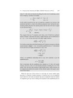
Figure 5.8. Market size and entry. The estimated .N; S/ relationships for (a) plumbers and
tire dealers and (b) doctors, chemists, and dentists. In each case, the vertical axis represents
the predicted number of firms in the market and the horizontal axis represents the market
size, measured in thousands of people. Authors’ calculations from the results in Bresnahan
and Reiss.
independent across observations, we can estimate this model as an ordered probit
model using maximum likelihood estimation.
23
The regression produces the estimated parameters that allow us to estimate the
variation of profitability with market size, variable profitability, and fixed profits.
Partial results, thosecapturing the determinants of variable profitability in the market
for doctors, are presented for illustration in table 5.6. Note that the results suggest
that there is a significant change in profitability between a monopoly and a duopoly
market. However, after three firms, further entry does not seem to change the average
profitability of firms.
From those results, we can retrieve the market size S
N
necessary for entry of
successive firms. We present the results in figure 5.8.
Looking first at the results for plumbers and tire dealers, the results suggest first
that plumbers never seem to have much market power no matter how many there
are. The estimated relationship between N and S is basically linear. In fact, the
23
For an econometric description of the model, see Maddala (1983). The model is reasonably easy
to program in Gauss or Matlab and the original Bresnahan and Reiss data set is available on the web
at the Center for the Study of Industrial Organization, www.csio.econ.northwestern.edu/data.html (last
verified May 2, 2007).
274 5. The Relationship between Market Structure and Price
results suggest that even a monopolist plumber does not have much market power,
though it may also be that there were not many markets with just one plumber

in. Somewhat in contrast, tire dealers appear to lose their monopoly rent with the
second entrant and thereafter the relationship between the number of players and
market size appears approximately linear as would be expected in a competitive
industry. The results for doctors, chemists, and plumbers and tire dealers appear to
fit Bresnahan and Reiss’s theory very nicely. Somewhat in contrast, in the dentist’s
results, while there is concavity until we observe two firms, the line for dentists
actually shows convexity after the third entrant, indicating that profitability increases
after the third entrant. Such a pattern could just be an artifact resulting from having
too little data at the larger market sizes, in which case it can be ignored as statistically
insignificant. However, it could also be due to idiosyncracies in the way dentist
practices are organized in bigger places and if so would merit further scrutiny to
make sure in particular that an important determinant of the entry decision for
dentists is not missing from the model. A problem that can arise in larger markets
is that the extent of geographic differentiation becomes a relevant factor and if so
unexpected patterns can appear in the .N; S/ relationship. If in such circumstances
the Bresnahan and Reiss model is not sufficient to model the data, then subsequent
authors have extended the basic model in a variety of ways: Berry (1992) to allow for
firm heterogeneity and Mazzeo (2002) and Seim (2006) extended the analysis and
estimation of entrygames to allow for product differentiation. Davis (2006c) allowed
for some forms of product differentiation and also in particular chain entry so that,
for example, each firm can operate more than one store and instead of choosing
0/1 firms choose 0;1;:::;N. Schaumans and Verboven (2008) significantly extend
Mazzeo’s model into an example of what Davis (2006c) called a “two-index” version
of these models. While most of the entry literature uses a pure strategy equilibrium
context suitable for a game of perfect information, Seim’s paper introduces the idea
that imperfect information (e.g., firms have private information about their costs)
may introduce realism to the model and also, fortuitously, help reduce the difficulties
associated with multiplicity ofequilibria. There is littledoubt that the class of models
developed in this spirit will continue to be extended and provide a useful toolbox
for applied work.

A striking general feature of Bresnahan and Reiss’s (1990) results is that they
find fairly consistently that market power appears to fall away at relatively small
market sizes, perhaps due to very relatively low fixed costs and modest barriers to
entry in the markets they considered. Although the results are limited to the data
they considered their study does provide us with a powerful tool for analyzing when
market power is likely to be being exploited and, at least as important, when it is
not.
The framework developed by Bresnahan and Reiss (1990) assumes a market
where firms are homogeneous and symmetric. This assumption serves to guarantee
5.2. Entry, Exit, and Pricing Power 275
that there is a unique optimal number of firms for a given market size. The method-
ology is not, however, able to predict the entry of individual firms or to incorporate
the effect of firm-specific sources of profitability such as a higher efficiency in a
given firm due to an idiosyncratic cost advantage. But, if we want to model entry
for heterogeneous firms, the resulting computational requirements become rather
greater and the whole process becomes more complex and therefore challenging on
an investigatory timetable. Sometimes such an investment may well be worthwhile,
but at present, generally, most applications of more sophisticated methods are at the
research and development stage rather than being directly applied in actual cases.
Although agencies have gone further than Bresnahan and Reiss in a relatively
small (tiny) number of cases, the subsequent industrial organization literature is
important enough to merit at least a brief introduction in this book. For example, if
an agency did want to allow for firm heterogeneity, then a useful framework is pro-
vided in Berry (1992). In particular, he argues persuasively that there are important
elements of both unobserved and observed firm heterogeneity in profitability, for
example, in terms of different costs, and therefore any model should account for it
appropriately. Many if not all firms, agencies, and practitioners would agree with the
principle that firms differ in important ways. Moreover, firm heterogeneity can have
important implications for the observed relationship between market size and the
number of firms. If the market size increases and efficient firms tend to enter first,

then we may observe greater concavity in the relationship between N and S. Berry
emphasizes the role of unobserved (to the econometrician) firm heterogeneity. In his
model the number of potential entrants plays an important role in telling us about
the likely role being played by unobserved firm heterogeneity. Specifically, if firm
heterogeneity is important we will actually tend to observe more actual entrants in
markets where there are more potential entrants for the same reason that the more
times we roll a die the more times we will observe sixes. For a review of some of
the subsequent literature see Berry and Reiss (2007).
5.2.4 What Do We Know about Entry?
Industrial organization economists know a great deal about entry and this book is
not an appropriate place to attempt to fully summarize what we know. However,
some broad themes do arise from the literature and therefore it seems valuable to
finish this chapter with a selection of those broad themes. First, entry and exit are
extremely important—and in general there is a lot of it. Second, it is sometimes
possible to spot characteristics of firms which are likely to make them particularly
likely entrants into markets, as any remedies section chief (in a competition agency)
will be able to tell you. Third, entry and exit are in reality often, but not exclusively,
best thought about as part of a process of growth and expansion, perhaps followed by
shrinking and exit rather than one-off events. This section reviews a small number
of the important papers on entry in the industrial organization literature. In doing so
276 5. The Relationship between Market Structure and Price
we aim to emphasize at least one important source of such general observations and
also to draw out both the modeling challenge being faced by those authors seeking to
generalize the Bresnahan and Reiss article and also to paint a picture of the dynamic
market environment in which antitrust investigations often take place.
5.2.4.1 Entry and Exit in U.S. Manufacturing
Dunne, Roberts, and Samuelson (1988) (DRS) present a comprehensive description
of entry and exit in U.S. manufacturing by using the U.S. Census of Manufactures
between 1963 and 1982. The census is produced every five years and has data from
every plant operated by every firm in 387 four-digit SIC manufacturing industries.

24
An example of a four-digit SIC classification is “metal cans,” “cutlery,” and “hand
and edge tools, except machine tools and handsaws,” which are all in the “fabricated
metal products” three-digit classification. In the early 1980s, a huge effort was
undertaken to turn these data into a longitudinal database, the Longitudinal Research
Database, that allowed following plants and firms across time. Many other countries
have similar databases, for example, the United Kingdom has an equivalent database
called the Annual Respondent Database.
The first finding from studying such databases is that there are sometimes very
high rates of entry and exit. To examine entry and exit rates empirically, DRS defined
the entry rate as the total number of new arrivals in the census in any given survey
year divided by the number of active firms in the previous survey year:
ENTRY RATE D
New arrivals this census
Active firms
t1
:
Similarly, DRS defined the exit rate as the total number of firms that exited since
the last survey year divided by the total number of firms in the last survey year:
EXIT RATE D
Exits since last census
Active firms
t1
:
Table 5.7 presents DRS’s results from doing so.
First note that the entry rate is very high, at least in the United States, on average
in manufacturing. Between 41 and 52% of all firms active in any given census year
are entrants since the last census, i.e., all those firms have entered in just five years!
Similarly, the exit rate is very high, indeed a similar proportion of the total number
of firms. Even ignoring entry and exit of smallest firms, the turnover appears to be

very substantial. On the other hand, if we examine the market share of entrants and
exitors, we see that on average entrants enter at a quarter to a fifth of the average
24
The Standard Industrial Classification (SIC) codes in the United States have been replaced by the
North American Industrial Classification System (NAICS) as part of the NAFTA process. The system
is now common across Mexico, the United States, and Canada and provides standard definitions at the
six-digit level compared with the four digits of the SIC (www.census.gov/epcd/www/naics.html). The
equivalent EU classification system is the NACE (Nomenclature statistique des Activit´es ´economiques
dans la Communaut´e Europ´eenne).
5.2. Entry, Exit, and Pricing Power 277
Table 5.7. Entry and exit variables for the U.S. manufacturing sector.
1963–67 1967–72 1972–77 1977–82
Entry rate (ER):
All firms 0.414 0.516 0.518 0.517
Smallest firms deleted 0.307 0.427 0.401 0.408
Entrant market share (ESH):
All firms 0.139 0.188 0.146 0.173
Smallest firms deleted 0.136 0.185 0.142 0.169
Entrant relative size (ERS):
All firms 0.271 0.286 0.205 0.228
Smallest firms deleted 0.369 0.359 0.280 0.324
Exit rate (XR):
All firms 0.417 0.490 0.450 0.500
Smallest firms deleted 0.308 0.390 0.338 0.372
Exiter market share (XSH):
All firms 0.148 0.195 0.150 0.178
Smallest firms deleted 0.144 0.191 0.146 0.173
Exiter relative size (XRS):
All firms 0.247 0.271 0.221 0.226
Smallest firms deleted 0.367 0.367 0.310 0.344

Source: Dunne et al.(1988, table 2).The table reportsentry and exit variables for the U.S. manufacturing
sector (averages over 387 four-digit SIC industries).
scale of existing firms in their product market and therefore account for only 14–
17% share of the total market between the years surveyed. Exiting firms have very
similar characteristics. The fact that entering and exiting firms are small gives us our
first indication that successful firms grow after entry but unless they maintain that
success, then they will shrink before eventually exiting. At the same time other firms
will never be particularly successful and they will enter small and exit small having
not substantively changed the competitive dynamics in an industry. Small-scale
entry will always feature in competition investigations, but claims by incumbents
that such small-scale entry proves they cannot have market power are usually not
appropriately taken at face value.
The figures in table 5.7 report the average (mean) rates for an individual man-
ufacturing industry and Dunne et al. also report that a large majority of industries
have entry rates of between 40 and 50%. Exceptions include the tobacco industry
with only 20% of entry and the food-processing industries with only 24%. They
found the highest entry rate in the “instruments” industry, which has a 60% entry
rate. Finally, we note that DRS find a significant correlation between entry and exit
measures, an observation we discuss further below.
278 5. The Relationship between Market Structure and Price
5.2.4.2 Identifying Potential Entrants
There are a number of ways to evaluate the set of potential entrants in a market.
Business school strategy teachers often propose undertaking a SWOT (strengths,
weaknesses, opportunities, and threats) analysis and such analyses do sometimes
make their way into company documents. After a company has undertaken such
an analysis, identified potential entrants will often be named under “threats,” while
markets presenting potential entry opportunities may be named in the opportunities
category. Thus information on potential entrants may come from company docu-
ments or, during an investigation, from surveys and questionnaires of customers
or rivals (who may consider backward integration), and/or senior managers (the

former may have the experience and skills necessary to consider setting up rival
companies). Alternatively, sometimes we can examine the issue empirically and in
this section we provide a couple of well-known examples of doing so.
First, let us return to Dunne et al., who found that the average firm produces in
more than one four-digit product classification and that single-plant firms account
for 93–95% of all firms but only 15–20% of the value of production. The latter figure
implies that multiplant firms account for an 80–85% share of total production. Such
observations suggest examining entry and exit rates by dividing potential entrants
into three types: new firms, diversifying firms entering the market with a new plant,
and diversifying firms entering the market using an existing plant.
Table 5.8 shows the entrants by type. Note that in any survey year, most entrants
are new firms opening new plants while diversifying firms opening a new plant
are a relatively rare event as it is much more common for diversifying firms to
enter by diversifying production at their existing plant. On the other hand, when a
diversifying firm enters with a new plant, it enters at a much larger scale than the
other entrant types, at a whopping 90% or more of the average size of the existing
firms in three of the survey years considered. Thus while entry by a multiproduct
firm opening a new plant is a relatively rare event, when it happens it will often
represent the appearance of a very significant new competitor.
For an example of how this can work, consider the U.K. Competition Commis-
sion’s analysis of the completed acquisition by Greif Inc. of the “new steel drum
and closures” business of Blagden Packaging Group, where new large-scale entry
played a very important role.
25
The CC noted that the merger, on its face, was likely
to result in a post-merger market share (of new large steel drums and closures in the
United Kingdom) of 85%, with the merger increment 32%. On the face of it, since
imports were negligible pre-merger, this merger clearly appeared to raise substan-
tial concerns unless there were some mitigating factors such as a very high demand
25

Closure systems are the mechanism by which the contents of a drum can be poured or pumped out
and the drum resealed. The CC found the market in closures was global so that the area of concern was
only steel drums. The CC (2007a) “found that, over the past five years, both Greif and Blagden lost more
custom to each other than to any other competitor in the world.”
5.2. Entry, Exit, and Pricing Power 279
Table 5.8. Entry variables by types of firms and method of entry.
Type of firm/
method of entry
a
1963–67 1967–72 1972–77 1977–82
Entry rate
Total 0.307 0.427 0.401 0.408
NF/NP 0.154 0.250 0.228 0.228
DF/NP 0.028 0.053 0.026 0.025
DF/PM 0.125 0.123 0.146 0.154
Entrant market share
Total 0.136 0.185 0.142 0.169
NF/NP 0.060 0.097 0.069 0.093
DF/NP 0.019 0.039 0.015 0.020
DF/PM 0.057 0.050 0.058 0.057
Entrant relative size
Total 0.369 0.359 0.280 0.324
NF/NP 0.288 0.308 0.227 0.311
DF/NP 0.980 0.919 0.689 0.896
DF/PM 0.406 0.346 0.344 0.298
a
NF/NP, new firm, new plant; DF/NP, diversifying firm, new plant; DF/PM, diversifying firm, product
mix. Source: Dunneet al. (1988, table 3). Entry variables by type of firm and method of entry.(Averages
over 387 four-digit SIC industries.)
elasticity. However, toward the end of the merger review process, a new entrant

building a whole new plant was identified: the Schuetz Group was constructing a
new plant at Moerdijk in the Netherlands, including a new steel drum production
line “with significant capacity.” The company described the facility as consisting of
a floorspace of 60,000 m
2
located strategically and ideally located between Rotter-
dam and Antwerp
26
with a capacity of 1.3 million drums annually per shift.
27
The
total U.K. sales of new large steel drums were estimated to be approximately 3.7
million in 2006.
28
This new entrant, whose plant was not operational at the time
of the CC’s final report, was deemed likely to become an important competitive
constraint on the incumbents once it did open at the end of 2007 or early 2008.
29
This appears to be one example of a diversifying firm entering a market by building
a new plant of significant scale, although the diversification is relative to the U.K.
geographic market rather than the activities of the firm per se.
26
A press release is available at www.schuetz.net/schuetz/en/company/press/industrial packaging/
english
articles/new location in moerdijk/index.phtml.
27
See paragraph 8.4 of CC (2007).
28
See table 2 of CC (2007).
29

In this case, Schuetz was already involved in some closely related products in the United Kingdom;
specifically, it was a U.K. manufacturer of intermediate bulk containers but not new large steel drums.
Schuetz was also already active in steel drums and a number of other bulk packaging products elsewhere
in the world.
280 5. The Relationship between Market Structure and Price
Table 5.9. Number and percentage of markets entered and exited in large cities by airlines.
#of #of #of %of %of
markets markets markets markets markets
Airline served entered exited entered exited
1 Delta 281 43 28 15.3 10.0
2 Eastern 257 33 36 12.8 14.0
3 United 231 36 10 15.6 4.3
4 American 207 22 12 10.6 5.8
5 USAir 201 20 17 10.0 5.8
6 TWA 174 22 23 12.6 13.2
7 Braniff 112 10 20 8.9 17.9
8 Northwest 75 6 7 8.0 9.3
9 Republic 69 9 6 13.0 8.7
10 Continental 62 9 5 14.5 8.1
11 Piedmont 61 14 2 23.0 3.3
12 Western 51 6 7 11.8 13.7
13 Pan Am 45 1 1 2.2 2.2
14 Ozark 28 18 4 64.3 14.3
15 Texas Int’l 27 3 6 11.1 22.2
Source: Berry (1992, table II). The number and percentage of markets entered and exited in the large
city sample by airline.
Interestingly, the fact that entry does not usually happen at the average scale
of operation for the industry is at least somewhat at odds with the assumption of
U-shaped average cost curves that predict that most firms should have approximately
the same efficient scale in the long run, as proposed in the influential Viner (1931)

cost structure theory of the size of the firm.
30
Indeed, one could in extremis argue
that these data seem to suggest that theory applies to only 2% of the data!
Berry (1992) provides an industry study where it proves possible to provide
evidence on the set of people who are likely to be potential entrants. He extensively
describes entry activity in the airline sector by using data from the “origin and
destination survey,” which comprises a random sample of 10% of all passenger
tickets issues by U.S. airlines. While Berry’s data involve only data from the first
and third quarters of 1980, it enables him to construct entry and exit data for that
relatively short period of nine months. Specifically, to look at entry and exit over the
period he constructs 1,219 “city-pair” markets linking the fifty major cities in the
United States. City-pair markets are defined as including tickets issued between the
two cities and do not necessarily involve direct flights, but (realistically) assuming
that the 10% ticket sample gives us a complete picture of the routes being flown, it
enables entry and exit data to be constructed (albeit under an implicitly broad market
definition where customers are willing to change planes). The results are provided in
table 5.9, which again reveals that there is a lot of entry and exit activity taking place.
30
See chapter 2 and, in particular, chapter 4 of Viner (1931), reprinted in Stigler and Boulding (1950).
5.2. Entry, Exit, and Pricing Power 281
Table 5.10. Joint frequency distribution of entry and exit in airline routes market.
Number of exits, as % of
total markets in the sample
Number of
‚
…„ ƒ
entrants (as %) 0 1 2 3+ Total
0 68.50 10.01 1.07 0.00 79.57
1 15.09 2.63 0.41 0.00 18.13

2 1.96 0.25 0.00 0.00 2.05
3+ 0.16 0.08 0.00 0.00 0.24
Total 85.56 12.96 1.48 0.00 100.00
Source: Berry (1992).
Table 5.11. Number of potential entrants by number of cities served
within a city pair, with number and percentage entering.
Total #
Number of of potential
cities served entrants # entering % entering
0 47,600 4 0.01
1 12,650 45 0.36
2 3,590 232 6.46
Source: Berry (1992).
Specifically, if we look at the results by markets, we see that entry and/or exit
occurred in more than a third of all markets, which implies significant dynamism
in the industry since this entry relates to only a nine-month period. Furthermore,
table 5.10 reports that 3.37% of markets, i.e., forty-one city-pair markets, expe-
rienced both entry and exit over these nine months. The existence of apparently
simultaneous entry and exit indicates that firm heterogeneity probably plays a role
in the market outcomes: some firms are better suited to compete in some of the
markets.
Berry (1992) examines whether airport presence in one of the cities makes an
airline carrier more likely to enter a market linking this city. He finds that this is
indeed the case. As illustrated in table 5.11, only rarely is there entry by someone
not already operating out of or into at least one of the cities concerned. In this case,
if one wants to estimate the likelihood of entry in the short term, potential entrants
should be defined as carriers that already operate in at least one of the cities.
To conclude this section, let us say that although the DRS study describes only
the manufacturing sector of the U.S. economy of the 1960s to the 1980s, the study
282 5. The Relationship between Market Structure and Price

remains both important and insightful more generally. In particular, it provides us
with a clear picture of the extensive amount of entry and exit that can occur within
relatively short time periods. If entry and exit drive competition, and most impor-
tantly productivity growth, then protecting that dynamic process will be extremely
important for a market economy to function, vital if the new entrants are drivers of
innovation. The facts thus outlined suggest in particular that while antitrust author-
ities can play a very important short-term or even medium-term role in considering
whether market concentrations shouldbe allowed to occur, the effectof an increase in
concentration which enhances market power may last only arelatively few years pro-
vided there are no substantial barriers to entry which act to keep out rivals attracted
by the resulting high profits. Making sure that profitable entry opportunities can
potentially be exploited by new or diversifying firms, i.e., ensuring efficient entrants
face at least a fairly level playing field, thus provides one of the most important
functions of competition policy.
5.3 Conclusions
 Most standard models of competition predict an effect of market structure on
the level of prices. Generally, all else equal, an increase in concentration or
a decrease in the number of firms operating in the market will be expected
to raise market prices and decrease output. In the case of firms competing in
prices of differentiated products which are demand substitutes, this effect is
unambiguously predicted by simple models. Whether such price rises/output
falls are in fact material, and whether all else is indeed equal, are therefore
central questions in most competition investigations involving changes in
market structure.
 One way to examine the quantitative effect of changes in market structure on
outcomes such as prices and output is to compare the outcomes of interest
across similarmarkets. The(impossible) idealis to find markets thatdifferonly
in the degree of concentration they exhibit. In reality we look for markets that
do not differ “too much” or in the “wrong way.” In particular, an analyst must
be wary of differing cost or demand characteristics of the different markets

and when interpreting such cross-market evidence an analyst must always
ask why otherwise similar markets exhibit different supply structures. In the
jargon of econometrics, cost and demand differences across markets that are
not controlled for in our analysis can result in our estimates suffering from
endogeneity problems. If so, then our observed correlation between market
structure and price is not indicative of a causal relationship but rather our
correlation is caused by an independent third factor.
5.3. Conclusions 283
 When the data allow, econometric techniques for dealing with the endogene-
ity problem can be very useful in attempting to distinguish correlations from
causality. Such techniques include the use of instrumental variables and fixed
effects. However, any technique for distinguishing two potential explanations
for the same phenomenon relies on assumptions for identifying which of
the contenders is in fact the true explanation. For example, when using the
fixed-effects technique, there must at a minimum be both (1) within-group
variation over time and (2) no other significant time-varying unobserved vari-
ables that are not accounted for in our analysis. The latter can be a problem,
in particular, when using identifying events over time such as entry by nearby
rivals. For example, sometimes prices rise following entry when firms seek
to differentiate their product offerings in light of that entry.
 Entry increases the number of firms in the market and, in an oligopoly setting,
is generally expected to lower prices and profitability in the market. Factors
which will affect whether we observe new entry may include expected prof-
itability for the entrant post entry, which in turn is determined by such factors
as the costs of entrants relative to incumbents, the potential size of the market,
and the erosion of market power due to the presence of additional firms. More-
over, incumbents can sometimes play strategic games to alter the perceived
or actual payoffs of potential entrants in order to deter entry.
 The economics literature emerging from static entry games has suggested
that the relationship between market size and the number of firms can be

informative about the extent of market power enjoyed by incumbents. To learn
about market power in this way, one must, however, make strong assumptions
about the static nature of competition. In particular, such analyses largely
consider entry as a “one-off” event, whereas entry is often best considered as
a “process” as firms enter on a small scale, grow when they are successful,
shrink when they are not, and perhaps ultimately exit.
 Relatedly, many markets are dynamic, experiencing a large amount of entry
and exit. A considerable amount of the observed entry and exit only involves
very small firms on the fringe of a market. However, a large number of mar-
kets do exhibit entry and exit over relatively short time horizons on a sub-
stantial scale. The existence of substantive entry and exit can alleviate the
concerns raised by actual, or, in the case of anticipated mergers, potential
market concentration. However, the importance of entry as a disciplining
device on incumbent firms also underlines the need for competition authori-
ties to preserve the ability of innovative and efficient new entrants to displace
inefficient incumbent firms.
6
Identification of Conduct
In the previous chapter, we discussed two major methods available for assessing the
effect of market structure on pricing and market power, the question at the heart of
merger investigations. The broader arena of competition policy is also concerned
with collusion by existing firms or the abuse of market power by a dominant firm.
For example, the U.S. Sherman Act (1890) is concerned with monopolization.
1
In
Europe, since the Treaty of Rome (1957) contains a reference to “dominant” firms,
collusion is known as the exercise of joint or collective dominance while the latter
is known as “single” dominance.
2
Any such case obviously requires a finding of

dominance and in order to determine whether a firm (or group of firms) is dominant
we need to know the extent of its individual (collective) market power.
In this chapter, we discuss methods for identifying the presence of market power
and in particular whether we can use data to discriminate between collusive out-
comes, dominant firm outcomes, competing firms acting as oligopolies, or outcomes
which sufficiently approximate perfect competition. That is, we ask whether we can
tell from market outcomes whether firms are imposing genuine competitive con-
straints on one another, or instead whether firms possess significant market power
and so can individually or collectively reduce output and raise prices to the detriment
of consumers.
Abuses of monopoly power (single dominance) are forbidden in European and
U.S. competition law. However, the range of abuses that are forbidden differs across
jurisdictions. In particular, in the EU both exclusionary (e.g., killing off an entrant)
and exploitative abuses (e.g., charging high prices) are in principle covered by com-
petition law while in the United States only exclusionary abuses are forbidden since
1
For a tour de force of the evolution of U.S. thinking on antitrust, see Shapiro and Kovacic (2000).
2
The term “dominant” appears in the Treaty of Rome, the founding treaty of the European Common
Market signed in 1957 and has played an important role in European competition policy ever since.
The term is unwieldy for most economists, as many are more familiar with cartels, monopolies, and
oligopolies. Today there are two relevant treaties which have been updated and consolidated into a
single document known as the consolidated version of the Treaty on European Union and of the Treaty
Establishing the European Community. This document was published in the Official Journal as OJ C. 321
E/1 29/12/2006. The latter treaty is a renamed and updated version of the Treaty of Rome. The contents
of Articles 81 and 82 of the treaty are broadly similar to the contents of the first U.S. antitrust act, the
Sherman Act (1890) as updated by the Clayton Act (1914). The laws in the European Union and the
United States differ, however, in some important areas. In particular, under the Sherman Act charging
monopoly prices is not illegal while under EU law, it can be. In addition, jurisprudence has introduced
differing legal tests for specific types of violations.

6.1. The Role of Structural Indicators 285
the Sherman Act states that to “monopolize, or attempt to monopolize,” constitutes
a felony but it does not say that to be a monopolist is a problem. The implication
is that a monopolist may, for example, charge whatever prices she likes so long
as dominant companies do not subsequently protect their monopolies by excluding
others who try to win business. In Europe, a monopolist or an industry collectively
charging prices that result in “excessive margins” could in principle be the subject
of an investigation.
When discussing collusion (joint dominance) it is important to distinguish
between explicit collusion (cartels) and tacit collusion, since the former is a criminal
offense in a growing number of jurisdictions. In Australia, Canada, Israel, Japan,
Korea, the United Kingdom, and the United States the worst forms of cartel abuses
are now criminal offenses so that cartelists may serve time in jail for their actions.
3
Events that increase the likelihood of explicit or tacit coordination are also closely
watched by competition authorities due to their negative effect on the competitive
process and consumer welfare. For example, a merger can be blocked if it is judged
likely to result in a “coordinated effect,” i.e., an increased likelihood of the industry
engaging in tacit collusion.
We begin our discussion of this important topic by first revisiting the history and
tradition of the “structure–conduct–performance” paradigm that dominated indus-
trial organization until the emergence of game theory. While such an approach is
currently widely regarded as old fashioned, we do so for two reasons. Firstit provides
a baseline for comparison with more recent work motivated primarily by static game
theory. Second, the movement toward analysis of dynamic games where evolution
of market shares may sometimes occur slowly over time, and empirical evidence
about early mover advantages in mature industries may, in the longer term, restore
the flavor of some elements of the structure–conduct–performance paradigm.
4
For

example, some influential commentators are currently calling for a return to a “struc-
tural presumption,” where, for example, more weight is given to market shares in
evaluating a merger (see, in particular, Baker and Shapiro 2007).
6.1 The Role of Structural Indicators
The structure–conduct–performance (SCP) framework—which presumes a causal
link between the structure of the market, the nature of competition, and market
3
U.S. cartelists have served jail time for many years since cartelization became a criminal offense
(in fact a felony) after the Sherman Act in 1890. Outside the United States, experience of criminal
prosecutions in this area is growing. Even where active enforcement by domestic authorities is limited,
in a number cases the very fact that legislation has passed criminalizing cartel behavior has enabled U.S.
authorities to pursue non-U.S. nationals in U.S. courts. The reason is that bilateral extradition treaties
sometimes require that the alleged offense is a criminal one in both jurisdictions.
4
See, for example, the work by Sutton (1991), Klepper (1996), and Klepper and Simons (2000), and
in the strategy literature see Markides and Geroski (2005) and McGahan (2004).
286 6. Identification of Conduct
outcomes in terms of prices, output, and profits—has a long history in industrial
organization. Indeed, competition policy relies on structural indicators for an initial
assessment of the extent of market power exercised by firms in a market. For exam-
ple, conduct or mergers involving small firms with market shares below a certain
threshold will normally not raise competition concerns. Similarly, mergers that do
not increase the concentration of a market above a certain threshold are assumed
likely to create minimal harm to consumers and for this reason we enshrine “safe
harbors” in law.
5
This provides legal certainty, the benefits of which may outweigh
any potential competitive damage. Those structural thresholds are useful to provide
some discriminating mechanism for competition authorities and allow them to con-
centrate on cases that are more likely to be harmful. However, “structural indicators”

such as market shares are now treated only, as the name emphasizes, as indicators
and are not considered conclusive evidence of market power. It is possible that the
pendulum will swing back slightly to place more presumptive weight on structure
in future years, though it is not clear it will do so at present. However, even if it does,
the lessons of static game theory that drive current practice and that we outline below
will remain extremely important. Most specifically, in some particular situations, a
high market share may provide an incumbent with very little market power.
6.1.1 Structural Proxies for Market Power
Most of the structural indicators that competition authorities consider when estab-
lishing grounds for an investigation or to voice concerns are derived from relation-
ships predicted by the Cournot model. For example, the reliance on market shares,
concentration ratios, and the importance attributed to the well-known Herfindahl–
Hirschman index (HHI) can each be theoretically justified using the static Cournot
model.
6.1.1.1 Economic Theory and the Structure–Conduct–Performance Framework
In antitrust, good information on marginal cost is rare, so it is often difficult to
directly estimate margins at the industry level to determine the presence of mar-
ket power. However, if we are prepared to make some assumptions we may have
alternative approaches. In particular, we may be able to use structural indicators to
infer profitability. For example, under the assumption that a Cournot game captures
the nature of competition in an industry, a firm’s margin is equal to the individual
market share divided by the market demand elasticity:
P.Q/ C
0
i
.q
i
/
P.Q/
D

s
i
Á
D
;
5
For a very nice description of the numerous market share thresholds enshrined in EU and U.K. law,
see Whish (2003).
6.1. The Role of Structural Indicators 287
where s
i
is the market share of the firm and Á
D
the market demand elasticity. Fur-
thermore, under Cournot, the weighted average industry margin is equal to the sum
of the squared individual market share divided by the market demand elasticity:
N
X
iD1
s
i
Â
P.Q/ C
0
i
.q
i
/
P.Q/
Ã

D
1
Á
D
N
X
iD1
s
2
i
:
To derive these relationships, recall that in the general Cournot first-order condition
for a market with several firms is
@
i
.q
i
;q
i
/
@q
i
D P
Â
N
X
j D1
q
j
Ã

C q
i
P
0
Â
N
X
j D1
q
j
Ã
 C
0
i
.q
i
/ D 0:
If we denote Q D
P
N
j D1
q
j
and we rearrange the first-order condition, we obtain
the firm’s markup index, also called the Lerner index, as a function of the firm’s
market share and the elasticity of the market demand:
P.Q/ C
0
i
.q

i
/
P.Q/
D q
i
P
0
.Q/
P.Q/
()
P.Q/ C
0
i
.q
i
/
P.Q/
D
q
i
Q
QP
0
.Q/
P.Q/
D
s
i
Á
D

:
This relationship can be used in a variety of ways. First, note that if we are
prepared to rely on the theory, the Cournot–Nash equilibrium allows us to retrieve
the markup of the firm using market share data and market demand elasticity. The
markup will be higher, the higher the market share of the firm. However, the markup
will decrease with the market demand elasticity. That means that a high market
share will be associated with a high markup, but that a high market share is not in
itself sufficient to ensure high markups. Even a high market share firm can have
no market power, no ability to raise price above costs if the market demand is
sufficiently elastic. An important fundamental implication is that while high market
shares are a legitimate signal of potential market power, high market shares should
not in themselves immediately translate into a finding of market power by antitrust
authorities. Naturally, measuring the nature of price sensitivity will be helpful in
determining if this is, in the particular case under consideration, a factually relevant
defense or just a theoretical argument.
There are estimates of average markups in many industries, often constructed
using publicly available data. Domowitz et al. (1988), for example, estimate average
margins for different industries in the United States using the Census of Manufac-
turing data and find that the average Lerner index for manufacturing industries in
the years 1958–81 is 0.37.
6.1.1.2 The Herfindahl–Hirschman Index and Concentration Ratios
There is a long tradition of inferring the extent of market power from structural indi-
cators of the industry. Firm size and industry concentration are the most commonly
288 6. Identification of Conduct
Table 6.1. HHI measures of market concentration: comparison of
CR(4) and HHI measures of market concentration.
Market 1 Market 2
‚
…„ ƒ‚…„ ƒ
Firm Share Share

2
Firm Share Share
2
1 20 400 1 50 2,500
2 20 400 2 20 400
3 20 400 3 5 25
4 20 400 4 5 25
5 20 400 5 5 25
—— — 6 5 25
CR(4) 80 CR(4) 80
HHI 2,000 HHI 2,950
used structural indicators of profitability and both are thought to be positively corre-
lated with market power and margins. The two most common indicators of industry
concentration are the K-firm concentration ratio and Herfindahl–Hirschman index
(HHI).
The K-firm concentration ratio (CR) involves calculation of the market shares of
the largest K firms so that
C
K
D
K
X
iD1
s
.i/
;
where s
.i/
is the ith largest firm’s market share.
The HHI is calculated using the sums of squares of market shares:

HHI D
N
X
iD1
s
2
i
;
where s
i
is the ith firm’s market share expressed as a percentage so that the HHI will
take values between 0 and 10,000 (D 100
2
). As illustrated above, in the Cournot
model, the HHI is proportional to industry profitability and can therefore be related
to firms’ market power.
The HHI will be higher if the structure of the market is more asymmetric. The
examples in table 6.1 show that the HHI is higher for a market in which there are
more firms but where one firm is very large compared with its competitors. Also,
given symmetry, a larger number of firms will decrease the value of the HHI.
The result that a market with few firms, or a market with one or two very big
firms, may be one where firms can exercise market power through high markups is
intuitive. As a result the HHI is used as a preliminary benchmark in merger control
where the data on a post-merger situation cannot be observed. Both U.S. and EU
merger guidelines use the HHI screen for mergers which are unlikely to be of much
6.1. The Role of Structural Indicators 289
concern and toflag those that shouldbe scrutinized. Thisis done by usingthe pre- and
post-merger market shares to compute the pre- and post-merger HHI. Respectively,
HHI
Pre

D
N
X
iD1
.s
Pre
i
/
2
and HHI
Post
D
N
X
iD1
.s
Post
i
/
2
;
where, since post-merger market shares are not observed and we need a practical
and easy-to-apply rule, post-merger market shares are assumed to simply be the
sum of the merging firms’ pre-merger market shares. In initial screening of mergers,
these values are assumed to be an indicator of the extent of margins before and after
the proposed merger and the effect of the merger on such margins. Specifically, in
the EU merger guidelines, mergers leading to the creation of a firm with less than
25% market share are presumed to be largely exempt from anticompetitive effects.
6
The regulations use an indicative threshold of 40% as being the point at which a

merger is likely to attract closer scrutiny.
7
Mergers that create a HHI index for the
market of less than 1,000 are also assumed to be clear of anticompetitive effects. For
post-merger HHI levels between 1,000 and 2,000, mergers that increase the HHI
level by less than 250 are also presumed to have no negative effect on competition.
Changes in the HHI index of less than 150 at HHI levels higher than 2,000 are
also declared to cause less concern except in some special circumstances. Similarly,
the U.S. Department of Justice Horizontal Merger Guidelines
8
also use a threshold
at 1,000, a region of 1,000–1,800 to indicate a moderately concentrated market,
and “where the post-merger HHI exceeds 1,800, it will be presumed that mergers
producing an increase in the HHI of more than 100 points are likely to create or
enhance market power or facilitate its exercise.”
To see these calculations in operation, next we present an example of the package
tour market using flights from U.K. origins. The first and second firms in the market,
Airtours and First Choice with 19.4% and 15% market shares respectively, merged
to create the largest firm in the industry with a combined 34.4% market share.
9
The
HHI index jumped from approximately1,982 before themerger to around2,564 after
the merger, an increase of 582. Such a merger would therefore be subject to scrutiny
under either the EU or U.S. guidelines. Of course, in using such screens, we can only
calculate market shares on the basis of a particular proposed market definition. In
practical settings, that often means there is plenty of room for substantial discussion
6
Guidelines on the assessment of horizontal mergers under the Council Regulation on the control
of concentrations between undertakings, 2004/C 31/3, Official Journal of the European Union C31/5
(5-2-2004).

7
Ibid. In the United Kingdom, the Enterprise Act 2002 empowers the OFT to refer mergers to the
CC if they create or enhance a 25% share of supply or where the U.K. turnover of the acquired firm is
over £70 million. As an aside, some argue that it is not immediately clear that the term “share of supply”
actually does mean the same as “market share.”
8
See the U.S. Horizontal Merger Guidelines available at www.usdoj.gov/atr/public/guidelines/
hmg.htm, section 1.5.
9
Airtours plc v. Commission of the European Communities, Case T-342/99 (2002).
290 6. Identification of Conduct
Table 6.2. HHI calculations for a merger in the package tour industry.
Adjustments
Company s
i
s
2
i
for merger
Airtours 19.4 376.36 376.36
First Choice 15.0 225 225
Combined 34.4 1,183.36 C1,183.36
Thomson 30.7 942.49
Thomas Cook 20.4 416.16
Cosmos Avro 2.9 8.41
Manos 1.7 2.89
Kosmar 1.7 2.89
Others (<1% each) 8.2 9 .8:2=9/
2
Total 100 1,982 2,564

Source: Underlying market share data are from Nielsen and quoted in table 1 from the European
Commission’s 1999 decision on Airtours v. First Choice. These calculations treat the market shares of
“Others” as being made up of nine equally sized firms, each with a market share of 8:2=9 D 0:83.
The exact assumption made about the number of small firms does not affect the analysis substantively.
over whether a merger meets these threshold tests even though lack of data means
it is not always possible to calculate even a precise HHI number so that results near
but on opposite sides of the thresholds are not appropriately treated as materially
different outcomes.
A practical disadvantage of the HHI is that it requires information on the volume
(or value) of sales of all companies, as distinct from a market share which requires
estimates of total sales and the sales of the main parties to a merger (the merging
companies). Competition agencies with powers to gather information from both
main and third parties may usually be able to compute HHI, at least to an acceptable
degree of approximation provided they can collect information from all the large
and moderately sized players. Very small companies will not usually materially
affect the outcome. On the other hand, some significant agencies (e.g., the Office
of Fair Trading in the United Kingdom) do not currently have powers to compel
information from third parties (while those which do may hesitate to use them) so
that even computing a HHI can sometimes face practical difficulties.
It is important to note that it is not the practice to prohibit a merger based on
HHI results alone. It is useful to use the HHI as a screening mechanism, but the
source of the potential market power should be understood before the measures
available to competition authorities are applied. That said, market shares and HHIs
will certainly play a role in the weighing up of evidence when deciding whether on
balance a merger is likely to substantially lessen competition.
6.1. The Role of Structural Indicators 291
Market structure
(market shares, HHI)
Firm conduct
(compete or collude)

Performance
(profits, welfare)
Structure
Conduct
Performance
Game-theory-informed
industrial organization
adds feedbacks
Figure 6.1. SCP versus game theory.
6.1.1.3 Beyond the SCP Framework
Theoretical developments in industrial organization, particularly static game theory,
clearly illustrated important limits of the SCP analysis. In particular, static game
theory suggests that the relationship between structure, conduct, and performance
is not generally best considered to be a causal relationship in a single direction.
In particular, the causality between market share and market power is in no way
automatically established. Even though the Cournot competition model predicts that
markups are linked to the market shares of the firms, it is very important to note that
high industry margins are not caused by high HHIs, even though they coincide with
high HHIs. Rather, in the Cournot model, concentration and price-cost markups are
both determined simultaneously in equilibrium. This means that they are ultimately
both determined by the strategic choices of the firms regarding prices, quantity, or
other variables such as advertising and by the structural parameters of the market,
particularly the nature of demand and the nature of technology which affects costs.
If the market demand and cost structure are such that optimization by individual
firms leads to a concentrated market, high margins may be difficult for even the
most powerful and interventionist competition agency to avoid. Under Cournot, for
example, firms that are low-cost producers will have high market shares because
they are efficient. Their higher markup is a direct result of their higher efficiency.
The pure SCP view of the world that structure actively determines conduct which
in turn determines performance has been subjected to a number of serious critiques.

In particular, as figure 6.1 illustrates, game theorists have argued that in the standard
static (one shot) economic models, market structure, conduct, and market perfor-
mance typically emerge simultaneously as jointly determined outcomes of a model
rather than being causally determined from each other. Such analyses suggest that a
useful framework for analysis is one that moves away from the simple SCP analysis,
where the link between structure and market power was assumed to be one-way and
deterministic, to one in which firms can endogenously choose their conduct and in
return affect the market structure.
292 6. Identification of Conduct
Although we have stressed the lack of established causality between structure and
performance in static models, it is important to note that many dynamic economic
models push considerably back in the other direction. For example, in the previous
chapter we examined the simplest two-stage models, where firms entered at the first
stage and then engaged in competition, perhaps in prices. In that model, structure—
in the sense of the set of firms that decided to enter—is decided at the first stage
and then does indeed determine prices at the second stage. A complete dismissal of
SCP analysis might therefore lead agencies in the wrong direction, but the extreme
version of SCP, the view that “structure” is enough to decide whether a merger
should be approved, is difficult to square with (at least) a considerable amount of
economic theory.
The importance of structural indicators in determining the extent of market power
and the anticompetitive effects of a merger has gradually decreased as the authorities
increasingly rely on detailed industry analysis for their conclusions. Still, structural
indicators remain important among many practitioners and decision makers because
of their apparent simplicityand their (sometimes misunderstood) linkwith economic
theory.
6.1.2 Empirical Evidence from Structure–Conduct–Performance
The popularity of the simple SCP framework lies in the fact that it provides a tool
for decision making based on data that are usually easily obtained. This has real
advantages in competition policy, not least because legal rules based on structural

criteria can provide a degree of legal certainty to parties considering how particular
transactions would be treated by the competition system. Critics, however, point
to disadvantages, particularly that certainty about the application of a simple but
inappropriate rule may leadto worse outcomes thanaccepting the ex ante uncertainty
that results from relying on a detailed investigation of the facts during a careful
investigation.
In considering the debate between the advocates and critics of SCP style analysis,
and its implications for the practice of competition policy, it is helpful to understand
an outline of the debate that has raged over the last sixty years within industrial
organization. We next outline that debate.
10
6.1.2.1 Structure–Conduct–Performance Regressions
SCP analysis received a substantial boost in the 1950s when the new census data in
the United States that provided information at the industry level were made avail-
able to researchers. These new data allowed empirical studies based on interindustry
10
For a classic survey of the profit–market power relationship and other empirical regularities
documented by authors writing about the SCP tradition, see Bresnahan (1989).