Quantitative Techniques for Competition and Antitrust Analysis by Peter Davis and Eliana Garcés_12 potx

408 8. Merger Simulation
p
1
p
2
p
2
NE
p
1
= R
1
( p
2
; c
1
)
*
p
2
= R
2
( p
1
; c
2
)
*
Price
Post-merger
(= Price

Cartel
)
Static ‘‘Nash equilibrium’’ prices
where each firm is doing the best
they can given the price charged
by the other(s)
p
1
= R
1
( p
2
; c
1
)
NE
p
2
= R
2
( p
1
; c
2
)
NE
p
1
NE
NE

NE
Figure 8.6. A two-to-one merger in a differentiated product pricing game.
the demand model. For example, the linear model could involve D
2
.p/ D a
2
C
b
21
p
1
Cb
22
p
22
so that @D
2
.p/=@p
1
D b
21
and, analogously, @D
1
.p/=@p
2
D b
12
.
Note that if the two products are substitutes and @D
i

.p/=@p
j
>0, then the equi-
librium price for a firm maximizing joint profits will be higher, absent countervailing
efficiencies. This is because the monopolist, unlike the single-product firm in the
duopoly, gains the profits from the customers who switch to the competing product
after a price increase. We illustrated this fact for the two-product game in chapter 2.
The effect of a merger in a two-to-one merger in a market with two differentiated
single-product firms is illustrated in figure 8.6. Because Bertrand price competition
with differentiated products is a model where products are strategic complements,
the reaction functions are increasing in the price of the other good. The intersection
of the two pricing functions gives the optimal price for the Bertrand duopoly. After
the merger, the firm will price differently since it internalizes the effect of changing
the price of a product on the other product’s profits. This will result in higher prices
for both products. In this case, the post-merger price is also that which would be
associated with a perfect cartel’s prices.
8.3.2.2 Multiproduct Firms
Let us now consider the case of a firm producing several products pre-merger. If a
market is initially composed of firms producing several products, this means that
firms’profit maximization already involves optimization across many products. The
pricing equation of given goods will also depend on the demand and cost parameters
of other goods which are produced by the same firm. A merger will result in a change
in the pricing equation of certain goods as the parameters of the cost and demand
of the products newly acquired by the firm will now enter the pricing equations of
8.3. General Model for Merger Simulation 409
all previously produced goods. This is because the number of products over which
the post-merger firm is maximizing profits has changed relative to the pre-merger
situation.
Suppose firmf producesa setof productswhich wedenote =
f

Â=Df1;:::;Jg
and which is unique to this firm. The set of products produced by the firm does not
typically include all J products in the market but only a subset of those. The profit-
maximization problem for this firm involves maximization of the profits on all the
goods produced by the firm:
max
p
f
X
j 2=
f
˘
j
.p
f
;p
f
/ D max
p
f
X
j 2=
f
.p
j
 mc
j
/D
j
.p/:

Solving for the profit-maximizing prices will result in a set of first-order conditions.
For firm f , the system of first-order conditions is represented as follows:
D
k
.p/ C
X
j 2=
f
.p
j
 mc
j
/
@D
j
.p/
@p
k
D 0 for all k 2=
f
:
To these equations, we must add the first-order conditions of the remaining firms
so that in the end we will, as before in the single-product-firms case, end up with a
total of J first-order conditions, one for each product being sold. Solving these J
equations for the J 1 vector of unknown prices p

will provide us with the Nash
equilibrium in prices for the game.
In comparison with the case where firms produced only a single product, the
first-order conditions for multiproduct firms have extra terms. This reflects the fact

that the firms internalize the effect of a change in prices on the revenues of the
substitute goods that they also produce. Because of differences in ownership, first-
order conditions may well not have the same number of terms across firms.
To simplify analysis of this game, we follow the literature and introduce a J J
ownership matrix  with the jkth element (i.e., j th row, kth column) defined by

jk
D
(
1 if same firm produces j and k;
0 otherwise:
We can rewrite the first-order conditions for each firm f D 1;:::;F as
D
k
.p/ C
J
X
j D1

jk
.p
j
 mc
j
/
@D
j
.p/
@p
k

D 0 for all k 2=
f
;
where the 
jk
terms allow the summation to be across all products in the market
in all first-order conditions for all firms. The matrix  acts to select the terms that
involve the products produced by firm f and changes with the ownership pattern
of products in the market. At the end of the day, performing the actual merger
simulations will only involve changing elements of this matrix from zero to one and
tracing through the effects of this change on equilibrium prices. Once again, we will
410 8. Merger Simulation
have a set of equations for every firm resulting in a total of J pricing equations, one
first-order condition for each product being sold.
In order to estimate demand parameters, we need to specify demand equations.
For simplicity, let us assume a system of linear demands of the form,
q
k
D D
k
.p
1
;p
2
;:::;p
J
/ D a
k
C
J

X
j D1
b
kj
p
j
for k D 1;:::;J:
This specification conveniently produces
@D
k
.p/
@p
j
D b
kj
:
So that the first-order conditions become
a
k
C
J
X
j D1
b
kj
p
j
C
J
X

kD1

jk
.p
j
 mc
j
/b
jk
D 0
for all k 2=
f
and for all f D 1;:::;F:
This will sometimes be written as
q
k
C
J
X
kD1

jk
.p
j
 mc
j
/b
jk
D 0 for all j; k D 1;:::;J
but one must then remember that the vector of quantities is endogenous and depen-

dent on prices. Writing the system of equations this way and adding it together
with the demand system provide the 2J equations which we could solve for the
2J endogenous variables: J prices and J quantities. Doing so provides the direct
analogue to the standard supply-and-demand system estimation that is familiar for
the homogeneous product case. Sometimes we will find it easier to work with only
J equations and to do so we need only substitute the demand function for each
product into the corresponding first-order condition. Doing so allows us to write a
J -dimensional system of equations which can be solved for the J unknown prices.
Large systems of equations are more tractable if expressed in matrix form. Fol-
lowing the treatment in Davis (2006d) to express the demand system in matrix form,
we need to define the matrix of demand parameters B
0
as
B
0
D
2
6
6
6
6
6
6
6
4
b
11
 b
1j
 b

1J
:
:
:
:
:
:
:
:
:
b
k1
 b
kj
 b
kJ
:
:
:
:
:
:
:
:
:
b
J1
 b
Jj
 b

JJ
3
7
7
7
7
7
7
7
5
;
8.3. General Model for Merger Simulation 411
where b
kj
D @D
k
.p/=@p
j
, and also define
a D
2
6
6
6
6
6
6
6
4
a

1
:
:
:
a
k
:
:
:
a
J
3
7
7
7
7
7
7
7
5
;
which is the vector of demand intercepts and where the prime on B indicates a
transpose. The system of demand equations can then be written as
2
6
6
6
6
6
6

6
4
q
1
:
:
:
q
k
:
:
:
q
J
3
7
7
7
7
7
7
7
5
D
2
6
6
6
6
6

6
6
4
a
1
:
:
:
a
k
:
:
:
a
J
3
7
7
7
7
7
7
7
5
C
2
6
6
6
6

6
6
6
4
b
11
 b
1j
 b
1J
:
:
:
:
:
:
:
:
:
b
k1
 b
kj
 b
kJ
:
:
:
:
:

:
:
:
:
b
J1
 b
Jj
 b
JJ
3
7
7
7
7
7
7
7
5
2
6
6
6
6
6
6
6
4
p
1

:
:
:
p
j
:
:
:
p
J
3
7
7
7
7
7
7
7
5
;
or, far more compactly in matrix form, as q D a CB
0
p.
In order to express the system of pricing equations in matrix format, we need to
specify the J J matrix  B, which is the element-by-element product of  and
B, sometimes called the Hadamard product.
15
Note that B is the transpose of B
0
.

Specifically, define
  B D
2
6
6
6
6
6
6
6
4

11
b
11
 
j1
b
j1
 
J1
b
J1
:
:
:
:
:
:
:

:
:

1k
b
1k

jk
b
jk

Jk
b
Jk
:
:
:
:
:
:
:
:
:

1J
b
1J
 
jJ
b

jJ
 
JJ
b
JJ
3
7
7
7
7
7
7
7
5
;
where b
jk
D @D
j
.p/=@p
k
. The rows will include the parameters of the pricing
equation of a given product k. The term 
jk
will take the value of either 1 or 0
depending on whether the firm produces goods j and k or not and 
jj
D 1 for all
j since the producer of good j produces good j .
Recall the analytic expression for the pricing equations:

D
k
.p/ C
J
X
j D1

jk
.p
j
 mc
j
/
@D
j
.p/
@p
k
D 0 for all k 2=
f
and for all =
f
:
The vector of all J first-order conditions can now be expressed in matrix terms as
a C B
0
p C.  B/.p  c/ D 0;
15
Such matrix products are easily programmed in most computer programs. For example, in Gauss
define A D B  C to define the Hadamard element-by-element product so that a

jk
D b
jk
c
jk
for
j D 1;:::;J and k D 1;:::;J.
412 8. Merger Simulation
where
c D
2
6
4
mc
1
:
:
:
mc
J
3
7
5
and a D
2
6
4
a
1
:

:
:
a
J
3
7
5
:
Alternatively, as we have already mentioned we may sometimes choose to work
with the J pricing equations without substituting the demand equations: q C . 
B/.p  c/ D 0. We will then need to work with a system of equations comprising
these J equations and also the J demand equations.
Written in matrix form, the equations that we need to solve simultaneously can
then compactly be written as
q C . B/.p  c/ D 0 and q D a C B
0
p:
Using a structural form specification with all endogenous variables on the left side
of the equations and the exogenous ones on the right side we have
"
.  B/ I
B
0
I
#"
p
q
#
D
"

.  B/ 0
.J J/
0
.J J/
I
.J J/
#"
c
a
#
;
which is equivalent to
"
p
q
#
D
"
.  B/ I
B
0
I
#
1
"
.  B/ 0
.J J/
0
.J J/
I

.J J/
#"
c
a
#
:
This expression gives an analytic solution for all prices and all quantities for any
ownership structure that can be represented in  since we may arbitrarily change
the values of 
jk
from 0s to 1s to change the ownership structure provided only
that we always respect the symmetry condition that 
jk
D 
kj
.
With this system in place, once the parameters in B, c, and a are known, we can
calculate equilibrium prices after a merger by setting the corresponding elements of

jk
to 1. Indeed, we can calculate the equilibrium prices and quantities (and hence
profits) for any ownership structure.
8.3.2.3 Example of Merger Simulation
To illustrate the method, consider the example presented in Davis (2006f), a market
consisting of six products that are initially produced by six different firms. Suppose
the demand for product 1 is approximated by a linear demand and its parameters
have been estimated as follows:
q
1
D 10  2p

1
C 0:3p
2
C 0:3p
3
C 0:3p
4
C 0:3p
5
C 0:3p
6
:
By a remarkably happy coincidence, the demands for other products have also been
estimated and conveniently turned out to have a similar form so that we can write
8.3. General Model for Merger Simulation 413
the full system of demand equations in the form
q
j
D 10  2p
j
C 0:3
X
k¤j
p
k
for j D 1;2;:::;6:
Let us assume marginal costs of all products are equal to 1 and that the merger will
generate no efficiencies so that c
Pre
j

D c
Post
j
D 1 for j D 1;2;:::;6.
The pricing equation for the single-product firm is derived from the profit
maximization first-order condition and takes the form
@˘.p
j
/
@p
j
D D
j
.p/ C .p
j
 c
j
/
@D
j
.p/
@p
j
D 0:
In our example this simplifies to
q
j
D .p
j
 c

j
/.2/:
The system of pricing and demand equations in the case of six firms producing one
product each is then written as a total of twelve equations:
"
.
Pre
 B/ I
B
0
I
#"
p
q
#
D
"
.
Pre
 B/ 0
.J J/
0
.J J/
I
.J J/
#"
c
a
#
;

where 
Pre
takes the form of the identity matrix and
B
0
D
2
6
6
6
6
6
6
6
4
2 0:3 0:3 0:3 0:3 0:3
0:3 2 0:3 0:3 0:3 0:3
0:3 0:3 2 0:3 0:3 0:3
0:3 0:3 0:3 2 0:3 0:3
0:3 0:3 0:3 0:3 2 0:3
0:3 0:3 0:3 0:3 0:3 2
3
7
7
7
7
7
7
7
5

;
.
Pre
 B/ D
2
6
6
6
6
6
6
6
4
200000
0 20000
002000
00020 0
000020
000002
3
7
7
7
7
7
7
7
5
;
c D

2
6
6
6
6
6
6
6
4
1
1
1
1
1
1
3
7
7
7
7
7
7
7
5
;aD
2
6
6
6
6

6
6
6
4
10
10
10
10
10
10
3
7
7
7
7
7
7
7
5
:
414 8. Merger Simulation
We can solve for prices and quantities:
"
p
q
#
D
"
.
Pre

 B/ I
B
0
I
#
1
"
.
Pre
 B/ 0
.J J/
0
.J J/
I
.J J/
#"
c
a
#
:
If the firm that produced product 1 merges with the firm that produced product 5 the
ownership matrix will change so that
.
Post-merger
 B/ D
2
6
6
6
6

6
6
6
4
2 0 0 0 0:3 0
0 20000
002000
00020 0
0:3 0 0 0 20
000002
3
7
7
7
7
7
7
7
5
:
This is because the new pricing equation for product 1 will be derived from the
following first-order condition:
@˘.p/
@p
1
D D
1
.p/ C .p
1
 c

1
/
@D
1
.p/
@p
1
C .p
5
 c
5
/
@D
5
.p/
@p
1
D 0;
which in our example results in
q
1
D .p
1
 c
1
/.2/  .p
5
 c
5
/.0:3/:

New equilibrium prices and quantities can then be easily calculated using the new
system of equations:
"
p
q
#
D
"
.
Post-merger
 B/ I
B
0
I
#
1
"
.
Post-merger
 B/ 0
.J J/
0
.J J/
I
.J J/
#"
c
a
#
:

These kinds of matrix equations are trivial to compute in programs such as Mat-
lab or Gauss. They may also be programmed easily into Microsoft Excel, making
merger simulation using the linear model a readily available method. The predicted
equilibrium prices for each product under different ownership structure are repre-
sented in table 8.1. The market structure is represented by .n
1
;:::;n
F
/, where the
length of the vector F indicates the total number of active firms in the market and
each of the values of n
f
represents the number of products produced by the f th
firm in the market. The largest firm is represented by n
1
. Tables 8.1 and 8.2 show
equilibrium prices and profits respectively for a variety of ownership structures. The
results show, for example, that a merger between a firm that produces five products
and one firm that produces one product, i.e., we move from market structure .5; 1/
to the market structure with one firm producing six products (6), increases the prices
by more than 33%. Table 8.2 shows that the merger is profitable.
8.3. General Model for Merger Simulation 415
Table 8.1. Prices under different ownership structures.
Market structure (n
1
;:::;n
F
)
‚
…„ ƒ

Product .1; 1; 1; 1; 1; 1/ .2; 2; 2/ .3; 3/ .4; 2/ .5; 1/ 6 (Cartel)
1 4.8 5.3 5.9 6.62 7.87 10.5
2 4.8 5.3 5.9 6.62 7.87 10.5
3 4.8 5.3 5.9 6.62 7.87 10.5
4 4.8 5.3 5.9 6.62 7.87 10.5
5 4.8 5.3 5.9 5.77 7.87 10.5
6 4.8 5.3 5.9 5.77 5.95 10.5
Table 8.2. Profits under different ownership structures.
Market structure .n
1
;:::;n
F
/
‚
…„ ƒ
Firms .1; 1; 1; 1; 1; 1/ .2; 2; 2/ .3; 3/ .4; 2/ .5; 1/ 6 (Cartel)
1 28.88 63.39 105 139 188.54 270.8
2 28.88 63.39 105 77.6 48.99
3 28.88 63.39
4 28.88
5 28.88
6 28.88
Industry profits 173 190 210 217 238 270.8
8.3.2.4 Inferring Marginal Costs
In cases where estimates of marginal costs cannot be obtained from industry infor-
mation, appropriate company documents, or management accounts, there is an
alternative approach available. Specifically, it is possible to infer the whole vec-
tor of marginal costs directly from the pricing equations provided we are willing
to assume that observed prices are equilibrium prices. Recall the expression for the
pricing equation in our linear demand example:

a C B
0
p C.  B/.p  c/ D 0:
In merger simulations, we usually use this equation to solve for the vector of prices
p. However, the pricing equation can also be used to solve for the marginal costs c
in the pre-merger market, where prices are known. Rearranging the pricing equation
we have
c D p C. B/
1
.a C B
0
p/:
More specifically, if we assumer pre-merger prices are equilibrium prices, then given
the demand parameters in .a; B/ and the pre-merger ownership structure embodied
416 8. Merger Simulation
in 
Pre
, we can infer pre-merger marginal cost products for every product using the
equation:
c
Pre
D p
Pre
C .
Pre
 B/
1
.a C B
0
p

Pre
/:
One needs to be very careful with this calculation since its accuracy greatly depends
on having estimated the correct demand parameters and also having assumed the
correct firm behavior. Remember that the assumptions made about the nature of
competition determine the form of the pricing equation. What we will obtain when
we solve for the marginal costs are the marginal costs implied by the existing prices,
the demand parameters which have been estimated and also the assumption about
the nature of competition taking place, in this case differentiated product Bertrand
price competition.
Given the strong reliance on the assumptions, it is necessary to be appropriately
confident that the assumptions are at least a reasonable approximation to reality. To
that end, it is vital to proceed to undertake appropriate reality checks of the results,
including at least checking that estimated marginal costs are actually positive and
ideally are within a reasonable distance of whatever accounting or approximate
measures of marginal cost are available. This kind of inference involving marginal
costs can be a useful method to check for the plausibility of the demand estimates and
the pricing equation. If the demand parameters are wrong, you may well find that the
inferred marginal costs come out either negative or implausibly large at the observed
prices. If the marginal costs inferred using the estimated demand parameters are
unrealistic, then this is a signal that there is often a problem with our estimates of
the price elasticities. Alternatively, there could also be problems with the way we
have assumed price setting works in that particular market.
8.3.3 General Linear Quantity Games
In this section we suppose that the model that best fits the market involves com-
petition in quantities. Further, suppose that firm f chooses the quantities of the
products it produces to maximize profits and marginal costs are constant, then the
firm’s problem can be written as
max
q

f
X
j 2=
f

j
.q
1
;q
2
;:::;q
J
/ D max
q
f
X
j 2=
f
.P
j
.q
1
;q
2
;:::;q
J
/  c
j
/q
j

;
where P
j
.q
1
;q
2
;:::;q
J
/ is the inverse demand curve for product j . The represen-
tative first-order condition (FOC) for product k is
J
X
j D1

kj
@P
j
.q/
@q
k
q
j
C .P
k
.q/ c
k
/ D 0:
We can estimate a linear demand function of the form q D a C B
0

p and obtain the
inverse demand functions
p D .B
0
/
1
q  .B
0
/
1
a:
8.3. General Model for Merger Simulation 417
In that case, the quantity setting equations become
.  .B
0
/
1
/q C p  c D 0:
And we can write the full structural form of the game in the following matrix
expression:
"
I .B
0
/
1
B
0
I
#"
p

q
#
D
"
I0
0I
#"
c
a
#
:
As usual, the expression that will allow us to calculate equilibrium quantities and
prices for an arbitrary ownership structure will then be
"
p
q
#
D
"
I .B
0
/
1
B
0
I
#
1
"
c

a
#
:
8.3.4 Nonlinear Demand Functions
In each of the examples discussed above, the demand system of equations had a
convenient linear form. In some cases, more complex preferences may require the
specification of nonlinear demand functions. The process for merger simulation in
this case is essentially unaltered. One needs to calibrate or estimate the demand
functions, solve for the pre-merger marginal costs if needed and then solve for the
post-merger predicted equilibrium prices. That said, solving for the post-merger
equilibrium prices is harder with nonlinear demands because it may involve solving
a J  1 system of nonlinear equations. Generally, and fortunately, simple iterative
methods such as the method of iterated best responses seem to converge fairly
robustly to equilibrium prices (see, for example, Milgrom and Roberts 1990).
Iterated best responses is a method whereby given a starting set of prices, the
best responses of firms are calculated in sequence. One continues to recalculate
best responses until they converge to a stable set of prices, the prices at which all
first-order conditions are satisfied. At that point, provided second-order conditions
are also satisfied, we will know we will have found a Nash equilibrium set of prices.
The process is familiar to most students used to working with reaction curves as
the method is often used to indicate convergence to Nash equilibrium in simple
two-product pricing games that can be graphed.
In practice, iterated best responses work as follows:
1. Define the best response for firm f given the rival’s prices as the price that
maximizes its profits under those market conditions:
R
f
.p
f
/ D argmax

p
f
X
j 2=
f
.p
j
 mc
j
/D
j
.p/:
2. Create the following algorithm (following steps 3–5) in a mathematical or
statistical package.
418 8. Merger Simulation
3. Pick a starting firm f =1 and a starting value for the prices of all products
p
0
D .p
0
f
;p
0
f
/:
Set k D 0.
4. For firm f , solve p
kC1
f
D R

f
.p
k
f
/ and set p
kC1
D .p
kC1
f
;p
k
f
/.
5. Iterate:
 if jp
kC1
 p
k
j <", then stop;
 else set k D k C 1 and f D
(
f C 1 if f<F;
1 otherwiseI
 go to step 4.
If the process converges, then all firms are setting p
k
f
D R
f
.p

k
f
/ and we have
by construction found a solution to the first-order conditions. Provided the second-
order conditions are also satisfied (careful analysts will need to check), we have also
found a Nash equilibrium.
In pricing games we do not need to use iterated best responses and typically a
large range of updating equations will result in convergence of prices to an equilib-
rium price vector. In the empirical literature, it has been common to use a simply
rearranged version of the pricing equation to find equilibrium prices. To ease presen-
tation of this result we will change notation slightly. Specifically, we denote demand
curves as q.p/ in order for D
p
q.p/ to denote the differential operator with respect
to p applied to q.p/. Specifically, denote the J J matrix of slopes of the demand
curves as D
p
q.p/ which has .j; k/th element, @q
j
.p/=@p
k
. Using the general form
of the first-order conditions for nonlinear demand curves, we can write our pricing
equations as
q.p/ CŒ  D
p
q.p/.p  c/ D 0;
where as before the “dot” denotes the Hadamard product. As a result the empirical
literature has often used the iteration
p

kC1
D c  Œ  D
p
q.p
k
/
1
q.p
k
/
to define a sequence of prices beginning from some initial value p
0
, often set equal
to c. In practice, for most demand systems used for empirical work, this iteration
appears to converge to a Nash equilibrium in prices. The closely related equation
c D p Œ D
p
q.p/
1
q.p/
can be used to define the value of marginal costs that are consistent with Nash prices
for a given ownership structure in a manner analogous to that used for the linear
demand curves case in section 8.3.2.4.
8.3. General Model for Merger Simulation 419
Iterated best responses do not generally work for quantity-setting games because
convergence is not always achieved due to the form of the reaction functions. There
are other methods of solving systems of nonlinear equations, but in general there are
good reasons to expect iterated best responses to work and converge to equilibrium
when best response functions are increasing.
16

As in most games, one should in theory check for multiple equilibria. Once we
have more than two products with nonlinear demands, the possible existence of
multiple equilibria may become a problem and, depending on the starting values
of prices, it is possible that we may converge to different equilibrium solutions.
That said, if there are multiple equilibria, supermodular game theory tells us that
in general pricing games among substitutes we will have “square” equilibrium sets.
One equilibrium will be the bottom corner, another will be the top corner, and if
we take the values of the other corners they will also be equilibria. This result is
referred to as the fact that equilibria in pricing games are “complete lattices” (i.e.,
squares).
17
If we think firms are good at coordinating, one may argue that the high
price equilibrium will be more likely. In that case, it may make sense to start the
process of iterating on best responses from a particularly high prices levels since
such sequences will tend to converge down to the high price and therefore high profit
equilibrium.
Even though it is good practice, it is by no means common practice to report
in great detail on the issue of multiple equilibria beyond trying the convergence to
equilibrium prices from a few initial prices and verifying that each time the algorithm
finds the same equilibrium.
18
8.3.5 Merger Simulation Applied
In this section, we describe two merger exercises that were executed in the context of
merger investigations by the European Commission. The discussion of these merger
simulations includes a brief description of the demand estimation that underlies the
simulation model, but we also refer the reader to chapter 9 for a more detailed
exploration of the myriad of interesting issues that may need to be addressed in that
important step of a merger simulation. The examples we present below illustrate
16
The reason is to do with the properties of supermodular games. See, for example, the literature cited in

Topkis (1998). In general, in any setting where we can construct a sequence of monotonically increasing
prices with prices constrained within a finite range, we will achieve convergence of equilibrium. For
those who remember graduate school real analysis, the underlying mathematical reason is that monotonic
sequences in compact spaces converge. Although, in general, quantity games cannot be solved in this
way, many such games can be (see Amir 1996).
17
See Topkis (1998) and, in particular, the results due to Vives (1990) and Zhou (1994).
18
Industrial economists are by no means unique in such an approach since the same potential for
multiplicity was, for example, present in most computational general equilibrium models and various
authors subsequently warned of the dangers of ignoring multiplicity in policy analysis. The computation
of general equilibrium models became commonplace following the important contribution by Scarf
(1973). The issue of multiplicity has arisen in applications. See, for example, the discussion in Mercenier
(1995) and Kehoe (1985).
420 8. Merger Simulation
what actual merger simulations look like and also provide examples of the type of
scrutiny and criticisms that such a simulation will face and hence the analyst needs
to address.
8.3.5.1 The Volvo–Scania Case
The European Commission used a merger simulation model for the first time in the
investigation of its Volvo–Scania merger during 1999 and 2000. Although the Com-
mission did not base its prohibition decision on the merger simulation, it mentioned
the fact that the results of the simulation confirmed the conclusions of the more
qualitative investigation.
19
The merger involved two truck manufacturers and the
investigation centered on five markets where the merger seemed to create a dom-
inant firm with a market share of more than or close to 50% in Sweden, Norway,
Finland, Denmark, and Ireland. Ivaldi and Verboven (2005) details the simulation
model developed for the case. The focus of the analysis was on heavy trucks, which

can be of two types known as “rigid” and “tractor,” the latter carrying a detachable
container.
The demand for heavy trucks was modeled as a sequence of choices by the
consumer, who in this case was a freight transportation company. Those companies
chose the category of truck they wanted and then the specific model within the
chosen category.
A model commonly used to represent this kind of nested choice behavior is the
nested logit model. In this case, because the data available were aggregate data, a
simple nested logit model was estimated using the three-stage least-squares (3SLS)
estimation technique (a description of this method can be found in general economet-
ric books such as, for example, Greene (2007), but see also the remarks below). The
nested logit model is worthy of discussion in and of itself and, while we introduce
the model briefly below for completeness, the reader is directed to chapter 9 and in
particular section 9.2.6 for a more extensive discussion. Here, we will just illustrate
how assumptions about customer choices underpin the demand specifications we
choose to estimate.
The nested logit model supposes that the payoff to individual i from choosing
product j is given by the “conditional indirect utility” function:
20
u
ij
D ı
j
C 
ig
C .1  /"
ij
;
where ı
j

is the mean valuation for product j which is assumed to be in nest, or
group, g. We denote the set of products in group g as G
g
. A diagram describing
19
Commission Decision of 14.03.2000 declaring a concentration to be incompatible with the common
market and the functioning of the EEA Agreement (Case no. COMP/M. 1672 Volvo/Scania) Council
Regulation (EEC) no. 4064/89.
20
This is termed the conditional indirect utility model because it is “conditional” on product j , while
it depends on prices (through ı
j
D˛p
j
C ˇx
j
C 
j
as explained further below). Direct utility
functions depend only on consumption bundles.
8.3. General Model for Merger Simulation 421
the nesting structure in this example is provided in figure 9.5. Note that "
ij
is
product-specific while 
ig
is common to all products within group g for a given
individual. The individual’s total idiosyncratic taste for product j is given by the
sum, 
ig

C.1/"
ij
. The parameter  takes a value between 0 and 1 and note that it
controls the extent to which a consumer’s idiosyncratic tastes are product- or group-
specific. If  D 1, the individual consumer’s idiosyncratic valuations for all the
products in a group are exactly the same and their preferences for each good in the
group g are perfectly correlated. That means, for example, that a consumer who buys
a good from group g will tend to be a consumer with a high idiosyncratic taste for all
products in group g. In the face of a price rise by the currently preferred good j , such
a consumer will tend to substitute toward another product in the same group since
she tends to prefer goods in that group. In Volvo–Scania the purchasers of trucks
were freight companies and if  is close to 1 it captures the taste that some freight
companies will prefer trucks to be rigid while others will prefer tractors, and in each
case freight companies will not easily shop outside their preferred group of products.
In contrast, if  D 0 and we make a judicious choice for the assumed distribution of

ig
, then the valuation of products within a group is not correlated and consumers
who buy a truck in a particular group will not have any systematic tendency to
switch to another product in that group.
21
They will compare models across all
product groups without exhibiting a particular preference for a particular group.
The average valuation ı
j
is assumed to depend on the price of the product p, the
observed characteristics of the product x
j
, and the unobserved characteristics of the
products 

j
that will play the role of product specific demand shocks. In particular,
a common assumption is that
ı
j
D˛p
j
C ˇx
j
C 
j
:
In this case, the observed product characteristics are horsepower, a dummy for
“nationally produced,” as well as country- and firm-specific dummies.
Normalizing the average utility of the outside good to 0, ı
0
D 0, and making usual
convenient assumptions about the distribution of the random terms, in particular,
that they are type 1 extreme value (see, for example, chapter 9, Berry (1994), or, for
the technically minded, the important contribution by McFadden (1981)), the nested
logit model produces the following expression for market shares, or more precisely
the probability s
j
that a potential consumer chooses the product j :
s
j
D
exp.ı
j
=.1  //D

1
g
D
g
.1 C
P
G
gD1
D
1
g
/
;
21
This is by no means obvious. We have omitted some admittedly technical details in the formulation
of this model and this footnote is designed to provide at least an indication of them. As noted in the
text, for this group-specific effect formulation to correspond to the nested logit model, we must assume a
particular distribution for 
ig
and moreover one that depends on the value of  so that it is more accurate
to write 
ig
./. In fact, Cardell (1997) shows that there is a unique choice of distribution for 
ig
such
that if "
ij
is an independent type I extreme value random variable, then 
ig
./ C .1  /"

ij
is also
an extreme value random variable provided 0 6 <1.
422 8. Merger Simulation
where
D
g
D
X
k2G
g
exp
Â
ı
k
1  
Ã
and the expression for ı
j
is provided above. The demand parameters to be estimated
are ˛, ˇ, and . To be consistent with the underlying theoretical assumptions of
the model it turns out that we need some parameters to satisfy some restrictions.
In particular, we need ˛>0and 0 6  6 1. We discuss this model at greater
length in chapter 9. For now we note one potentially problematic feature of the
nested logit model: the resulting product demand functions satisfy the assumption
of “independence of irrelevant alternatives” (IIA) within a nest. IIA means that if
an alternative is added or subtracted in a group, the relative probability of choosing
between two other choices in the group is unchanged. This assumption was heavily
criticized by the opposing experts in the case.
The data needed for the estimation are the prices for all products, the charac-

teristics of the products, and the probability that a particular good is chosen. This
probability is approximated by the product market share so that
s
j
D
q
j
M
;
where q
j
is the quantity sold of good j and M is the total number of potential
consumers. The market share needs to be computed taking into account the outside
good, which is why the total number of potential consumers and not the total number
of actual buyers is in the denominator. Ivaldi and Verboven assume that the potential
market is either 50% or 300% larger than the actual sales. A potential market that is
50% larger than market sales can be described as M D 1:5.
P
J
j D1
q
j
/.
Ivaldi and Verboven (2005) linearize the demand equations using a transformation
procedure proposed by Berry (1994). We refer the reader to the detailed discussion
of that transformation procedure in chapter 9, for now noting that this procedure
means that estimating the model boils down to estimation of a linear model using
instrumental variables. In addition, the authors assume a marginal cost function
which is constant in quantity and which depends on a vector of observed cost shifters
w

j
and an error term. The observed cost shifters included horsepower, a dummy
variable for “tractor truck,” a set of country-specific fixed effects, and a set of firm-
specific fixed effects. The marginal cost function is assumed to be of the form,
c
j
D exp.w
j
 C !
j
/;
where  is a vector of parameters to be estimated, w
j
denotes a vector of observed
cost shifters and !
j
represents a determinant of marginal cost that is unobserved
by the econometrician and which will play the role of error terms in the pricing
(supply) equations (one for each product). As we have described numerous times in
this chapter, the profit of each firm f can be written as

f
D
X
j 2=
f
.p
j
 c
j

/q
j
.p/  F;
8.3. General Model for Merger Simulation 423
where =
f
is the subset of product produced by firm f , c
j
is the marginal cost of
product j , which is assumed to be constant, and F are the fixed costs. The Nash
equilibrium for a multiproduct firm in a price competition game is represented by
the set of j pricing equations:
q
j
C
X
k2=
f
.p
k
 c
k
/
@q
k
@p
j
D 0:
Replacing the marginal cost function results in the pricing equation:
q

j
C
X
k2=
f
.p
k
 exp.w
j
 C !
j
//
@q
k
@p
j
D 0 for j 2=
f
and also for each firm f:
These J equations, together with the J demand equations, provide us with the
structural form for this model. Note that the structural model involves a demand
curve and a “supply” or pricing equation for each product available in the market,
a total of 2J equations. The only substantive difference between the linear and this
nonlinear demand curve case is that these supply (pricing) and demand equations
must be solved numerically in order to calculate equilibrium prices for given values
of the demand- and cost-side parameters and data.
The data used to estimate the model covered two years of sales from truck com-
panies in sixteen European countries. To estimate the model, we use identification
conditions based on the two error terms of the model. Specifically, we assume that
at the true parameter values, EŒ

j
.ˇ

;

/ j z
1j
 D 0 and EŒ!
j
.ˇ

;

/ j z
2j
 D 0
(where z
1j
and z
2j
are sets of instrumental variables) in order to identify the demand
and supply equations.These moment conditions are exactly analogousto the moment
conditions imposed on demand and supply shocks in the homogeneous product con-
text.
22
Ivaldi and Verboven undertake a simultaneous estimation of the demand and
pricing equations using a nonlinear 3SLS procedure. While in principle at least the
demand side could be estimated separately, the authors use the structure to impose
all the cross-equation parameter restrictions during estimation. The sum of horse-
power of all competing products in a country per year and the sum of horsepower

of all competing products in a group per year are used as instruments to account for
the endogeneity of prices and quantities in both the demand and pricing equation
following the approach suggested initially by Berry et al. (1995). The technique
they use, 3SLS, is a well-known technique for estimation of simultaneous equation
22
The analyst may on occasion find it appropriate to estimate such a model using 2J moment con-
ditions, one for each supply (pricing) and demand equation. Doing so requires us to have multiple
observations on each product’s demand and pricing intersection, perhaps using data variation over time
from each product (demand and supply equation intersection). Alternatively, it may be appropriate to
estimate the model using only these two moment conditions and use the cross-product data variation
directly in estimation. This approach may be appropriate when unobserved product and cost shocks are
largely independent across products or else the covariance structure can be appropriately approximated.
424 8. Merger Simulation
Table 8.3. Estimates of the parameters of interest.
Potential market factor
‚
…„ ƒ
r D 0:5 r D 3:0
‚
…„ ƒ‚ …„ ƒ
Estimates Standard error Estimates Standard error
˛ 0.312 0.092 0.280 0.094
 0.341 0.240 0.304 0.240
Source: Table 2 from Ivaldi and Verboven (2005).
models. The first two stages of 3SLS are very similar to 2SLS while in the Ivaldi–
Verboven formulation the third stage attempts to account for the possible correlation
between the random terms across demand and pricing equations.
Estimation produces results consistent with the theory such as the fact that firm-
specific effects that are associated with higher marginal costs produce higher valua-
tions for consumers. Horsepower also increases costs. On the other hand, the authors

find that horsepower has a negative albeit insignificant effect on customer valuation.
The authors explain this by arguing that the higher maintenance costs associated with
higher horsepower may lower the demand but the result is nevertheless somewhat
troubling. The authors also report that they obtain positive and reasonable estimates
for marginal costs and mean product valuations. The estimated marginal costs imply
margins which were higher than those obtained in reality, although this observation
was a criticism rejected by the authors on the grounds that accounting data do not
necessarily reflect economic costs.
Table 8.3 shows the results for a subset of the demand parameters, namely ˛ and
, for two scenarios regarding the size of the total potential market. Specifically,
r D 0:5 corresponds to M D 1:5.
P
J
j D1
q
j
/ while r D 3:0 describes a potential
market size 300% greater than the actual market size. The parameter  is positive
and less than 1 but insignificantly different from 0, which means that the hypothesis
that rigid and tractor trucks form a single group of products cannot be rejected. Since
the hypothesis that  D 1 can be rejected, the hypothesis of perfect correlations
in idiosyncratic consumer tastes across the various trucks within a group can be
rejected.
Ivaldi and Verboven (2005) calculate the implied market demand elasticities for
the two different potential market size scenarios. The larger the potential market
size, the larger is the estimated share of the outside good and the higher is the
implied elasticity. The reason is that the outside option has a higher likelihood—by
construction. Estimating a large outside option produces a large market demand
elasticity and therefore a smaller estimate of the effect of the merger. The higher
elasticity was therefore chosen to predict the merger effect. Analysts using merger

8.3. General Model for Merger Simulation 425
simulation models, or evaluating merger simulation models presented by the parties’
expert economists, must be wary of apparently reasonable assumptions that are
driving the results to be those desired for the approval of a merger.
Once the parameters for the demand, cost, and pricing equations are estimated
for the pre-merger situation, post-merger equilibrium prices are computed using a
specification of the pricing equations that takes into account the new ownership
structure. That is, as before we change the definition of the ownership matrix, .
The new system of demand function and pricing equations, for which estimates of
all the parameters are now known, needs to be solved numerically to obtain equilib-
rium prices and quantities. Equilibrium prices and quantities were also computed
assuming a 5% reduction in marginal costs to simulate the potential effect of merger
synergies on the resulting prices. The resulting estimated price increases are not
duplicated here. Since the model is built on an explicit model of consumer utilities,
we may use the model to calculate estimates of consumer surplus with and with-
out the merger. The study finds that two countries—Sweden and Norway—would
experience decreases in consumer welfare higher than 10% and three additional
countries—Denmark, Finland, and Ireland—would each have consumer surplus
declines larger than 5%. Finland, Norway, and Sweden were predicted to have con-
sumer welfare decreases of more than 5% even in the event of a 5% reduction in
marginal costs.
8.3.5.2 The Lagard`ere–VUP Case
A similar model was used in the context of the Lagard`ere–VUP case investigated
by the European Commission in 2003, and this time the results of the simulation
were cited in the arguments supporting the decision.
23
The merger was subsequently
approved undersome divestment conditions. The caseinvolved theproposed acquisi-
tion by French group Lagard`ere, owner of the second largest publisher in the market,
Hachette, of Vivendi Universal Publishing (now Editis), the largest publisher in the

market. Foncel and Ivaldi performed the merger simulation for the Commission.
24
In this simulation, consumer preferences were also modeled using the nested logit
model. The nesting structure involved consumers first choosing the genre of the book
they wanted to buy (novel, thriller, romance, etc.) and then choosing a particular
title.
The data used were from a survey of sales of the 5,000 pocket books and the 1,500
large books with the highest sales. The data included sales by type of retailer, prices,
format, pages, editor, and title and author information. Only the general literature
23
Commission Decision of 7.01.2004 declaring a concentration compatible with the common market
and the functioning of the EEA Agreement (Case COMP/M.2978 Lagard`ere/Natexis/Vivendi Universal
Publishing) Council Regulation (EEC) no. 4064/89. See paragraphs 700–707.
24
“Evaluation Econom´etrique des Effets de la Concentration Lagard`ere/VUP sur le March´eduLivre
de Litt´erature G´en´erale,” J´erˆome Foncel et Marc Ivaldi, revised and expanded final version, September
2003.
426 8. Merger Simulation
titles were considered for the study. The total potential size of the market, M in the
notation above, was defined as the number of people in the country that do not buy
a book in the year plus the number of books sold during that year. The explanatory
variables for both the demand and the cost function were the format of the book,
the pages in the book, the purchase place, and measures of the authors’ and editors’
reputations.
The instruments chosen were versions of the observed variables such as the format
of other books in the same category and the number of competing products, again
following the approach suggested by Berry et al. (1995). Instruments are supposed
to affect either the supply (pricing) equation or the demand but not both. To correctly
identify the demand parameters, one must have at least one instrumental variable per
demand parameter to be estimated on an endogenous variable that affects the supply

of that product but not the demand. With the particular demand structure used in
this case, if only price is treated as an endogenous variable and instrumented in the
demand model and moreover price enters linearly in the conditional indirect utility
model, then we need only one instrument to estimate the demand side in addition
to the variables which explain demand and which are treated as exogenous (e.g., in
this case the book characteristics). As in the previous case, the experts worked with
aggregate data and estimated the parameters of the model using 3SLS. Based on the
estimates obtained, they computed the matrix of own- and cross-price elasticities,
the marginal costs, and therefore obtained the predicted margins.
To simulate the effect of the merger, the pricing equations were recalculated given
the new ownership structure and the predicted equilibrium prices were calculated.
The merger simulation estimated price increases of more than 5% for a market size
smaller than 100 million. The merger simulation was also conducted assuming an
ownership structure that incorporated remedies in the form of disinvestments by the
new merged entity.
In addition to calculating the predicted price increase, the authors built a confi-
dence interval for the estimated price increase using a standard bootstrap methodol-
ogy. To do so, they sampled 1,000 possible values of parameters using their estimated
distribution and calculated the corresponding price increases. Doing so allowed them
to calculate an estimate of the variance of the predicted price increase.
8.4 Merger Simulation: Coordinated Effects
The use of merger simulation has been generally accepted in the analysis of unilat-
eral effects of mergers. In principle, we can use similar techniques to evaluate the
effect of mergers on coordinated effects. Kovacic et al. (2007) propose using the
output from unilateral effects models to evaluate both competitive profits and also
collusive profits and thereby determine the incentive to collude. The authors argue
that such analyses can be helpful in understanding when coordination is likely to
8.4. Merger Simulation: Coordinated Effects 427
take place since firms can be innovative when finding solutions to difficult coor-
dination problems if the incentives to do so are large enough (Coase 1988). Davis

(2005) and Sabbatini (2006) each independently also argue that the same methods
used to analyze unilateral effects in mergers can be informative about the way a
change in market structure affects the incentives to coordinate.
25
However, they
take a broader view of the incentives to collude and propose evaluating each of the
elements of the incentive to collude that economic theory has isolated, following the
classic analysis in Friedman (1971).
26
Staying close to the economic theory allows
them to use simulation models to help inform investigators about firms’ ability to
sustain coordination, and in particular how that may change pre- and post-merger.
In Europe, the legal environment also favors such an approach since the Airtours
decision explicitly linked the analysis of coordinated effects to the economic theory
of coordination.
27
We follow their discussion in the rest of this section and refer the
reader to Davis and Huse (2008) for an empirical example applying these methods
in the network server market.
8.4.1 Theoretical Setting
The current generation of simulation models that can be used to estimate the effect
of mergers on coordinated effects rests on the same principles as the use of merger
simulation in a unilateral effect setting. Each type of simulation model uses the
estimates of the parameters in the structural model to calculate equilibrium prices
and profits under different scenarios. Whereas in the simulation of unilateral effect,
one need only calculate equilibrium under different ownership scenarios, in a coor-
dinated effect setting, one must also calculate equilibrium prices and profits under
different competition regimes, in a sense we make precise below.
8.4.1.1 Three Profit Measures from the Static Game
Firms face strong incentives to coordinate to achieve a higher prices, but when the

higher prices prevail each firm usually finds it has an incentive to cheat to get a
higher share of the profits generated by the higher price. This incentive to cheat may
therefore undermine the strong incentive to collude.
Friedman (1971) suggested that to analyze the sustainability and therefore the
likelihood of collusion one must evaluate the ability to sustain collusion and that is
related to the incentives of each firm to do so. That in turn suggests that we need
25
These authors have now combined working papers into a joint paper (Davis and Sabbatini 2009).
26
Important theoretical contributions are currently being made. For the differentiated product context,
see, most recently, K¨uhn (2004).
27
Airtours Plc v. Commission of the European Communities, Case no. T342-99. The Commission’s
decision to block the Airtours merger with First Choice in 1999 was annulled by the European Court
of First Instance (CFI) in June 2002. In the judgment the CFI outlined what have become known as the
“Airtours” conditions building largely on the conventional economic theory of collusion.
428 8. Merger Simulation
to attempt to estimate, or at least evaluate, each of the three different measures of
profit outlined above and which we now describe further:
(i) Own competitive profits 
Comp
f
are easily calculated for all firms using the
prices derived from the Nash equilibrium formula derived in our study of
unilateral effects merger simulation.
(ii) Own fully collusive profits 
Coll
f
may also be calculated using the results from
unilateral effects merger simulation for the case where all products are owned

by a single firm. Having used that method to calculate collusive prices, each
firm’s achieved share of collusive profits can be computed. Doing so means
that firms will obtain profits from all the products in their product line but not
those produced by rival firms. Because firms’ product lines are asymmetric,
the individual firm’s collusive profits will not generally correspond to simply
total industry profits divided by the number of firms.
(iii) Economic theory suggests that a firm’s own defection profits 
Def
f
should be
calculated by setting all rival firms’ prices to their collusive levels and then
determining the cheater’s own best price by finding the prices that maximize
the profit the firm can achieve by undercutting rivals and boosting sales given
their rivals’ collusive prices and before their rivals discover that a firm is
cheating. Capacity constraints may be an important issue and, as we show
below, can be taken into account as a constraint in the profit-maximization
exercise.
Specifically, consider a collusive market where rivals behave so as to maximize total
industry profits and set prices at the cartel level. A defector firm f will choose its
price to maximize its own profits from the goods it sells and will therefore fulfill the
following first-order condition for maximization:
max
fp
j
jj 2=
f
g
X
j 2=
f

.p
j
 c
j
/D
j
.p
f
;p
Coll
f
/;
where j is a product in the set =
f
of products produced by firm f . Firm f chooses
the set of prices p
f
for all the goods j 2=
f
it produces at its profit-maximizing
levels. The prices of all products from all firms except those of firm f are set at
collusive levels.
If capacity utilization is high and firms face limits on the extent to which they
can expand their output, we can include a capacity constraint restriction of the form
D
j
.p
f
;p
Coll

f
/ 6 Capacity
j
.
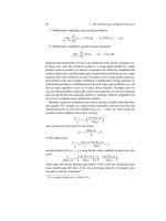
The competitive Nash equilibrium price, the collusive price, and the defection
price are each represented in figure 8.7 for the case of a two-player game. The prices
for defection are selected to fulfill p
Def
2
D R
2
.p
Coll
1
Ic
2
/ and p
Def
1
D R
1
.p
Coll
2
Ic
1
/.
8.4. Merger Simulation: Coordinated Effects 429
p
2

p
1
p
2
Coll
p
2
Def
p
2
NE
p
1
= R
1
( p
2
; c
1
)
*
p
1
NE
p
1
Def
p
1
Coll

p
2
= R
2
( p
1
; c
2
)
*
Static ‘‘Nash
equilibrium’’ prices
Price
Coll
Figure 8.7. Depiction of the competitive Nash equilibrium price, the collusive
price, and the defection price for a two-player pricing game. Source: Davis (2006f).
8.4.1.2 Comparing Payoffs
Now that we have defined the static payoffs under the different firm behaviors,
we will need to construct the dynamic payoffs for a multiperiod game given the
strategies being played. The economics of collusion rely on dynamic oligopoly
models. To solve for equilibrium strategies in a dynamic game, we must specify the
way in which firms will react if they catch their competitors cheating on a collusive
arrangement. In such models, equilibrium strategies will be dynamic. One standard
dynamic strategy that can sustain equilibria of the dynamic game is known as “grim
strategies.” Davis and Sabbatini (2009) use that approach and so assume that if a firm
defects from a cartel, the market will revert to competition in all future successive
periods.
If firms follow “grim strategies,” then the cartel will be sustainable if there are
no incentives to defect, which requires that the expected benefits from collusion be
higher than the expected benefits from defection.

Formally, following Friedman (1971), the firm’s incentive compatibility constraint
can be written as
V
Coll
f
D

Coll
f
1  ı
>
Def
f
C
ı
Comp
f
1  ı
D V
Cheat
f
;
where ı is the discount factor for future revenue streams (and which may be firm-
specific and if so should be indexed by f ). This inequality follows from subgame
perfection, which requires that in collusive equilibrium firms must prefer to coor-
dinate whenever they have the choice not to. Davis and Huse (2008) estimate each
firm’s discount factor ı using the working average cost of capital (WACC), which
430 8. Merger Simulation
in turn is computed using the debt-equity structure of the firm together with esti-
mates of the cost of debt finance and the cost of equity finance. The cost of debt

can be observed from listed firms using their reported interest costs together with
information on their use of debt finance. The cost of equity can be estimated using
an asset pricing model such as CAPM which uses stock market data. To illustrate
the potential importance of this, note that they found Dell to have an appreciably
lower discount factor than other rivals, perhaps in light of the uncertainties dur-
ing the data period arising from investor concern about the chance of success of
its direct-to-consumer business strategy. Factors such as the rate of market growth
and the chance of discovery by competition authorities may well be important to
incorporate into these incentive compatibility constraints.
In multiperiod games, the incentives to tacitly coordinate will depend on the
discount factor. The exact shape of the inequality will also depend on the strategies
being used to support collusion. For instance, there may be a possibility to return to
coordination after a period of punishment or there may not. If there is a punishment
period, then we will also wish to calculate the net present value of the returns to the
firm during the punishment period since that will enter the incentive compatibility
constraint. (We will have another incentive compatibility constraint arising from the
need for strategies followed during the punishment periods to be subgame perfect,
although we know these incentive constraints are automatically satisfied under a
punishment regime involving Nash reversion such as occurs when firms follow
grim strategies.)
Next we further consider the example we looked at earlier in the chapter (see
section 8.3.2.3 and in particular tables 8.1 and 8.2, which reported prices and profits
in Nash equilibrium for a variety of market structures for the example) in which
six single-product firms face a linear symmetric demand system. An example of the
payoffs to defection under different ownership structures in the one-period game is
presented in table 8.4. In our example, firms are assumed to have the same costs and
demand and are therefore symmetric in all but product ownership structure. As we
described above, the profits when a firm defects is calculated using the defection
prices for the defecting firms and the cartel prices for the remaining firms. Without
loss of generality, the table reports the results when firm 1 is the defector and the

other firms set their prices at collusive levels.
Table 8.5 presents the net present value payoffs under both collusion and defection
when defection is followed by a reversion to competition. Results are shown for
different assumptions for the value of the discount factor and for two different market
structures. With a zero discount factor, the firms completely discount the future
and so the model is effectively a unilateral effects model. As the discount factor
increases, future profits become more valuable and collusion becomes relatively
more attractive. In the example with market structure = .1; 1; 1; 1; 1; 1/ so that there
are six single-product firms, the critical discount factor is about 0.61. Collusion is
8.4. Merger Simulation: Coordinated Effects 431
Table 8.4. One-period payoffs to defection and collusion.
Collusive
Market payoffs
structure/ under
firm .1; 1; 1; 1; 1; 1/ .2; 2; 2/ .3; 3/ .4; 2/ .5; 1/ 6 (Cartel) cartel
1 70.50 128.47 174.50 210.00 238.30 270.75 45.12
2 34.97 52.03 57.05 31.17 19.74 45.12
3 34.97 52.03 45.12
4 34.97 45.12
5 34.97 45.12
6 34.97 45.12
Firm 1: one-period defection payoffs after defection 
Def
f
.
Source: Davis (2006f).
Table 8.5. The value of collusion and cheating under the two market structures.
Market structure Market structure
= .1; 1; 1; 1; 1; 1/ = .2;2;2/
‚

…„ ƒ‚ …„ ƒ
ıV
Coll
V
Cheat
V
Coll
V
Cheat
0 45.1 70.5 90 128
0.1 50.1 73.7 100 136
0.2 56.4 77.7 113 144
0.3 64.4 82.9 129 156
0.4 75.2 89.8 150 171
0.5 90.2 99.4 180 192
0.6 112.8 113.8 226

224
0.7 150.4

137.8 301

276
0.8 225.6

186.0 451

382
0.9 451.2


330.4 902

699
0.99 4,512.4

2,929.0 9,025

6,405
Source: Davis (2006f).

Denotes IC constraint satisfied.
sustainable for all discount factors higher than this value. Unsurprisingly, this is
consistent with the general theoretical result that cartels are more sustainable with
high discount factors, i.e., when income in the future is assigned a higher value.
We can calculate the critical discount factor for different market structures. To do
so, the second set of figures correspond to a post-merger market structure where a
total of three symmetric mergers have occurred, producing three firms each produc-
ing two products. Considering such a case, while a little unorthodox, is useful as
a presentational device because it ensures that firms are symmetric post-merger as
432 8. Merger Simulation
well as pre-merger, thus ensuring that every firm faces an identical incentive com-
patibility constraint before the merger and also afterward. This helps to present the
results more compactly. The before-and-after incentives to collude are, of course,
different from one another and, in fact, the critical discount factor after which col-
lusion is sustainable with the new more concentrated market structure is reduced to
just below 0.6, compared with 0.61 before the mergers.
For collusion to be an equilibrium, the incentive compatibility constraint must
hold for every single active firm. In the example discussed, the firms are symmetric so
all will fulfill this condition at the same time. For merger to generate a strengthening
of coordinated effects, the inequality must hold in some sense “more easily” for all

or some firms after the merger than it did before the merger. One way to think about
“more easily” is to say coordination is easier post-merger if the inequality holds for
a broader range of credible discount factors. On the other hand, Davis and Huse
(2009) show that for a given set of discount factors, mergers will generically (1) not
change perfectly collusive profits, (2) increase Nash profits, and (3) either leave
unchanged defection profits (nonmerging firms) or increase them (merging firms).
Since perfectly collusive profits are unchanged while (2) and (3) mean that the
defection payoffs generally increase, the result suggests that mergers will generally
make the incentive compatibility constraint for coordination harder to satisfy.
8.4.2 Merger Simulation Results for Coordinated Effects
The next two tables show numerical examples of the effect of mergers on the incen-
tives to tacitly coordinate. We first note that the results confirm that asymmetric
market structures can be bad for sustaining collusion. Table 8.6, for instance, shows
that if the market has one large firm producing five products and one small firm
producing one product, collusion will never be an outcome unless there is a sys-
tem of side payments to compensate the smaller firm. In the table, stars denote
situations where the incentive compatibility constraint (ICC) suggests that tacit
coordination is preferable for that firm. This result from Davis (2006f) establishes
that a “folk” theorem—which, for example, suggests that in homogeneous product
models of collusion there will always exist a discount factor at which collusion
can be sustained—do not universally hold in differentiated product models under
asymmetry.
Table 8.7 presents two examples of merger simulation from three to two firms.
Suppose the pre-merger market structure involves one firm producing four products
and two firms producing one product each, denoted by the market structure .4;1;1/.
The ICCs for the four-product firm and the (two) one-product firms are shown in the
last four columns of table 8.7. Tacit coordination appears sustainable if both firms
ICCs are satisfied, which occurs if discount factors are above 0.8. First suppose that
the larger firm acquires a smaller firm making the post-merger market structure .5; 1/
and second suppose that in the other case the two smaller firms merge making the