Báo cáo sinh học: " Research Article Analysis and Numerical Solutions of Positive and Dead Core Solutions of Singular Sturm-Liouville Problems" pptx
Bạn đang xem bản rút gọn của tài liệu. Xem và tải ngay bản đầy đủ của tài liệu tại đây (2.44 MB, 37 trang )
Hindawi Publishing Corporation
Advances in Difference Equations
Volume 2010, Article ID 969536, 37 pages
doi:10.1155/2010/969536
Research Article
Analysis and Numerical Solutions of
Positive and Dead Core Solutions of
Singular Sturm-Liouville Problems
Gernot Pulverer,
1
Svatoslav Stan
ˇ
ek,
2
and Ewa B. Weinm
¨
uller
1
1
Institute for Analysis and Scientific Computing, Vienna University of Technology,
Wiedner Hauptstrasse 6-10, 1040 Vienna, Austria
2
Department of Mathematical Analysis, Faculty of Science, Palack
´
y University, Tomkova 40,
779 00 Olomouc, Czech Republic
Correspondence should be addressed to Svatoslav Stan
ˇ
ek,
Received 20 December 2009; Accepted 28 April 2010
Academic Editor: Josef Diblik
Copyright q 2010 Gernot Pulverer et al. This is an open access article distributed under the
Creative Commons Attribution License, which permits unrestricted use, distribution, and
reproduction in any medium, provided the original work is properly cited.
In this paper, we investigate the singular Sturm-Liouville problem u
λgu, u
00, βu
1
αu1A,whereλ is a nonnegative parameter, β ≥ 0, α>0, and A>0. We discuss the existence
of multiple positive solutions and show that for certain values of λ, there also exist solutions that
vanish on a subinterval 0,ρ ⊂ 0, 1, the so-called dead core solutions. The theoretical findings
are illustrated by computational experiments for gu1/
√
u and for some model problems from
the class of singular differential equations φu
ft, u
λgt, u, u
discussed in Agarwal et al.
2007. For the numerical simulation, the collocation method implemented in our MATLAB code
bvpsuite has been applied.
1. Introduction
In the theory of diffusion and reaction see, e.g., 1, the reaction-diffusion phenomena are
described by the equation
Δv φ
2
h
x, v
,
1.1
where x ∈ Ω ⊂ R
N
.Herev ≥ 0 is the concentration of one of the reactants and φ is the Thiele
modulus. In case that h is radial symmetric with respect to x, the radial solutions of the above
2 Advances in Difference Equations
equation satisfying the boundary conditions
β
δv
δn
αv A
1.2
are solutions to a boundary value problem of the type
u
t
f
t, u
t
φ
2
h
t, u
t
,
u
0
0,βu
1
αu
1
A, β ≥ 0,α,A>0,
1.3
where t denotes the radial coordinate. Baxley and Gersdorff2 discussed problem 1.3,
where f and h were continuous and h was allowed to be unbounded for u → 0
. They
proved the existence of positive solutions and dead core solutions vanishing on a subinterval
0,t
0
,0<t
0
< 1 of problem 1.3, and also covered the case of the function h approximated
by some regular function h
κ
.
Problem 1.3 was a motivation for discussing positive, pseudo dead core, and dead
core solutions to the singular boundary value problem with a φ-Laplacian,
φu
t
f
t, u
t
λg
t, u
t
,u
t
,λ>0,
1.4a
u
0
0,βu
T
αu
T
A, β ≥ 0,α,A>0, 1.4b
see 3.Hereλ is a parameter, the function f is non-negative and satisfies the Carath
´
eodory
conditions on 0,T × 0, ∞, ft, 00 for a.e. t ∈ 0,T,andg is positive and satisfies the
Carath
´
eodory conditions on 0,T ×D, D 0,A/α × 0, ∞. Moreover, the function ft, x
is singular at t 0andgt, x, y is singular at x 0.
Let us denote by AC
loc
0,T the set of functions x : 0,T → R which are absolutely
continuous on ε, T for arbitrary small ε>0.
A function u ∈ C
1
0,T is called a positive solution of problem 1.4a-1.4b if u>0on
0,T, φu
∈ AC
loc
0,T, u satisfies 1.4b and 1.4a holds for a.e. t ∈ 0,T. We say that
u ∈ C
1
0,T satisfying 1.4b is a dead core solution of problem 1.4a-1.4b if there exists a
point ρ ∈ 0,T such that u 0on0,ρ, u>0onρ, T, φu
∈ ACρ, T and 1.4a holds
for a.e. t ∈ ρ, T. The interval 0,ρ is called the dead core of u.Ifu00, u>0on0,T,
φu
∈ AC
loc
0,T, u satisfies 1.4b and 1.4a holds a.e. on 0,T, then u is called a pseudo
dead core solution of problem 1.4a-1.4b.
Since problem 1.4a-1.4b is singular, the existence results in 3 are proved by a
combination of the method of lower and upper functions with regularization and sequential
techniques. Therefore, the notion of a sequential solution of problem 1.4a-1.4b was
introduced. In 3, conditions on the functions φ, f,andg were specified which guarantee
that for each λ>0, problem 1.4a-1.4b has a sequential solution and that any sequential
solution is either a positive solution, a pseudo dead core solution, or a dead core solution.
Also, it was shown that all sequential solutions of 1.4a-1.4b are positive solutions for
sufficiently small positive values of λ and dead core solutions for sufficiently large values
of λ.
Advances in Difference Equations 3
The differential equation 1.5a of the following boundary value problem satisfies all
conditions specified in 3:
u
t
γ
u
t
t
ρ
λ
1
u
t
u
t
ν
, 1.5a
u
0
0,αu
1
βu
1
1,α>0,β>0. 1.5b
Here, γ,ρ ∈ 0, ∞,andν ∈ 0,γ 1. We note that in papers 2, 3 no information on the
number of positive and dead core solutions of the underlying problem is given.
In this paper, we discuss the singular boundary value problem
u
t
λg
u
t
,λ≥ 0, 1.6a
u
0
0,αu
1
βu
1
1,α>0,β>0, 1.6b
where λ is a non-negative parameter, and the function g ∈ C0, ∞ becomes unbounded at
u 0. Problem 1.6a-1.6b is the special case of problem 1.4a-1.4b.
A function u ∈ C
2
0, 1 is a positive solution of problem 1.6a-1.6b if u satisfies the
boundary conditions 1.6b, u>0on0, 1 and 1.6a holds for t ∈ 0, 1.Afunctionu :
0, 1 → 0, ∞ is called a dead core solution of problem 1.6a-1.6b if there exists a point
ρ ∈ 0, 1 such that ut0fort ∈ 0,ρ, u ∈ C
1
0, 1 ∩ C
2
ρ, 1, u satisfies 1.6b and 1.6a
holds for t ∈ ρ, 1. The interval 0,ρ is called thedeadcoreof u.Ifρ 0, then u is called a
pseudo dead core solution of problem 1.6a-1.6b.
The aim of this paper is twofold.
1 First of all, we analyze relations between the values of the parameter λ and the
number and types of solutions to problem 1.6a-1.6b, provided that
g ∈ C
0, ∞
,gis positive, lim
u →0
g
u
∞,
a
0
g
s
ds<∞∀a>0
1.7
or
g ∈ C
1
0, ∞
,gis positive and decreasing, lim
u →0
g
u
∞,
a
0
g
s
ds<∞∀a>0.
1.8
4 Advances in Difference Equations
2 Moreover, we compute solutions u to the singular boundary value problem
u
t
λ
u
t
,λ≥ 0,
1.9a
u
0
0,αu
1
βu
1
1,α>0,β>0, 1.9b
and the singular problem 1.5a, 1.9b.Notethat1.9a is the special case of 1.6a
with g satisfying 1.8.
In 4 similar questions in context of 1.6a and the Dirichlet boundary conditions
u01, u11 have been discussed. For further results on existence of positive and dead
core solutions to differential equations of the types u
λgt, u and φu
gt, u, u
,we
refer the reader to 5–9. The Dirichlet conditions have been discussed in 5–7, 9, while 8
deals with the Robin conditions −u
−1αu−1a, u
1αu1a, α, a>0.
We now recapitulate the main analytical results formulated in Theorems 2.10, 2.12,and
2.13. First, we introduce the auxiliary function
H
x, y
:
⎧
⎪
⎪
⎨
⎪
⎪
⎩
αy β
y
x
ds
s
x
g
v
dv
y
x
g
v
dv, 0 ≤ x<y,
αy, 0 ≤ x y,
1.10
where g satisfies 1.7.ByLemma 2.2, the equation Hx, γx 1 has a unique continuous
solution γ ∈ C0, 1/α, and the function
χ
x
:
⎧
⎪
⎪
⎪
⎨
⎪
⎪
⎪
⎩
γx
x
ds
s
x
g
v
dv
,x∈
0,
1
α
,
0,x
1
α
1.11
is continuous on 0, 1/α.LetM : {χx
2
/2:0<x≤ 1/α}. Then the following statements
hold.
i Problem 1.6a-1.6b has a positive solution if and only if λ ∈M. In addition, for
each a ∈ 0, 1/α, problem 1.6a-1.6b with λ χa
2
/2hasauniquepositive
solution such that u0a, u1γa.
ii Problem 1.6a-1.6b has a pseudo dead core solution if and only if
λ
1
2
⎛
⎜
⎝
γ0
0
ds
s
0
gvdv
⎞
⎟
⎠
2
.
1.12
This solution is unique.
Advances in Difference Equations 5
iii Problem 1.6a-1.6b has a dead core solution if and only if
λ>
1
2
⎛
⎜
⎝
γ0
0
ds
s
0
gvdv
⎞
⎟
⎠
2
.
1.13
In addition, for all such λ, problem 1.6a-1.6b has a unique dead core solution.
The final result concerning the multiplicity of positive solutions to problem 1.6a-
1.6b is given in Theorem 2.11.Let1.8 hold and let Γ : max{τ : τ ∈M}. Then Γ >
χ0
2
/2 and for each λ ∈ χ0
2
/2, Γ, there exist multiple positive solutions of problem
1.6a-1.6b.
In Section 2 analytical results are presented. Here, we formulate the existence and
uniqueness results for the solutions of the boundary value problem 1.6a-1.6b and study
the dependance of the solution on the parameter values λ. The numerical treatment of
problems 1.9a-1.9b and 1.5a-1.5b based on the collocation method is discussed in
Section 3, where for different values of λ, we study positive, pseudo dead core, and dead
core solutions of problem 1.9a-1.9b and positive solutions of problem 1.5a-1.5b.
2. Analytical Results
2.1. Auxiliary Functions
Let assumption 1.7 hold, and let us introduce auxiliary functions ϕ
a
,H,andh as
ϕ
a
x
:
⎧
⎪
⎪
⎨
⎪
⎪
⎩
x
a
ds
s
a
g
v
dv
,x∈
a, ∞
,
0,x a,
2.1
where a ∈ 0, ∞,
H
x, y
:
⎧
⎪
⎪
⎨
⎪
⎪
⎩
αy β
y
x
ds
s
x
g
v
dv
y
x
g
v
dv, 0 ≤ x<y,
αy, 0 ≤ x y,
2.2
h
t, y
: αy
β
1 − t
y
0
ds
s
0
g
v
dv
y
0
g
v
dv,
t, y
∈
0, 1
×
0, ∞
.
2.3
Here, the positive constants α and β are identical with those used in boundary conditions
1.6b. Note that the function H is used in the analysis of positive and pseudo dead core
solutions of problem 1.6a-1.6b, while the function h for its dead core solutions.
Properties of ϕ
a
are described in the following lemma.
Lemma 2.1. Let assumption 1.7 hold and let a ∈ 0, ∞.Thenϕ
a
∈ Ca, ∞ ∩ C
1
a, ∞, and ϕ
a
is increasing on a, ∞.
6 Advances in Difference Equations
Proof. Let c be arbitrary, c>a. Then ϕ
a
∈ Ca, c ∩ C
1
a, c,andϕ
a
is increasing on a, c by
4, Lemma 2.3 where 1 is replaced by c. Since c>ais arbitrary, the result immediately
follows.
In the following lemma, we introduce functions γ and χ and discuss their properties.
Lemma 2.2. Let assumption 1.7 hold. Then the following statements follow.
i The function H is continuous on Δ{x, y ∈ R
2
:0≤ x ≤ y}, and ∂H/∂yx, y > 0
for 0 ≤ x<y.
ii For each x ∈ 0, 1/α, there exists a unique γx ∈ a, 1/α such that
H
x, γ
x
1 for x ∈
0,
1
α
, 2.4
and γ ∈ C0, 1/α, γx >xfor x ∈ 0, 1/α, γ1/α1/α.
iii The function
χ
x
:
⎧
⎪
⎪
⎪
⎨
⎪
⎪
⎪
⎩
γx
x
ds
s
x
g
v
dv
,x∈
0,
1
α
,
0,x
1
α
2.5
is continuous on 0, 1/α.
Proof. i Let us define S, P on Δ by
S
x, y
:
y
x
g
v
dv,
P
x, y
:
⎧
⎪
⎪
⎨
⎪
⎪
⎩
y
x
ds
s
x
g
v
dv
, 0 ≤ x<y,
0, 0 ≤ x y.
2.6
Then S ∈ CΔ.Letx ≥ 0anddefinem : min{gs :0<s≤ x 1}. Then, by 1.7, m>0.
Hence
0 <
y
x
ds
s
x
g
v
dv
≤
1
√
m
y
x
ds
√
s − x
2
y − x
m
,y∈
x, x 1
,
2.7
Advances in Difference Equations 7
and consequently lim
x,y∈Δ,y →x
Px, y0, which means that P is continuous at x, x.Let
0 ≤ x
0
<y
0
. We now show that P is continuous at the point x
0
,y
0
. Let us choose an arbitrary
y
∗
in the interval x
0
,y
0
. Then Px, yI
1
xI
2
x, y for x ∈ 0,y
∗
and y>y
∗
, where
I
1
x
y
∗
x
ds
s
x
g
v
dv
,I
2
x, y
y
y
∗
ds
s
x
g
v
dv
.
2.8
Since I
1
∈ C0,y
∗
by 4, Lemma 2.1 where 1 was replaced by y
∗
, it follows that I
1
is
continuous at x x
0
. The continuity of P at x
0
,y
0
now follows from the fact that I
2
is
continuous at this point. Hence P is continuous on Δ,andfromHx, yαyβPx, ySx, y
we conclude H ∈ CΔ. Since
∂H
∂y
x, y
α β
βq
y
2
y
x
g
v
dv
y
x
ds
s
x
g
v
dv
, 0 ≤ x<y,
2.9
we have ∂H/∂yx, y > 0for0≤ x<y.
ii Consider the equation Hx, y1, that is,
αy β
y
x
ds
s
x
g
v
dv
y
x
g
v
dv
1.
2.10
The function Hx, · is increasing on x, ∞, H1/α, 1/α1, and, for x ∈ 0, 1/α,
Hx, 1/α > 1. Hence, for each x ∈ 0, 1/α, there exists a unique γx such that Hx, γx
1andγ1/α1/α. Clearly, γx >xfor x ∈ 0, 1/α. In order to prove that γ ∈ C0, 1/α
,
suppose the contrary, that is, suppose that γ is discontinuous at a point x x
0
, x
0
∈ 0, 1/α.
Then there exist sequences {ν
n
}, {μ
n
} in 0, 1/α such that lim
n →∞
ν
n
x
0
lim
n →∞
μ
n
,and
the sequences {γν
n
}, {γμ
n
} are convergent, lim
n →∞
γν
n
c
1
, lim
n →∞
γμ
n
c
2
, c
1
/
c
2
.
Let n →∞in Hν
n
,γν
n
1andinHμ
n
,γμ
n
1. This means Hx
0
,c
j
1, j 1, 2,
and c
1
c
2
γx
0
by the definition of the function γ, which contradicts c
1
/
c
2
.
iii By ii,
αγ
x
βχ
x
γx
x
g
v
dv 1,x∈
0,
1
α
,
2.11
γ ∈ C0, 1/α and γx >xfor x ∈ 0, 1/α. Hence, the function
γx
x
gvdv is continuous
on 0, 1/α and positive on 0, 1/α.From
χ
x
1 − αγ
x
β
γx
x
g
v
dv
,x∈
0,
1
α
,
2.12
8 Advances in Difference Equations
we now deduce that χ ∈ C0, 1/α. Since
χ
x
≤
1
√
m
γx
x
ds
√
s − x
2
γ
x
− x
m
,x∈
0,
1
α
,
2.13
where m : min{gu :0<u≤ 1/α} > 0, and χ>0on0, 1/α, γ1/α1/α, we conclude
lim
x →1/α
−
χx0. Hence χ is continuous at x 1/α, and consequently γ ∈ C1, 1/α.
Let γ be the function from Lemma 2.2ii defined on the interval 0, 1/α.Fromnow
on, Λ denotes the value of γ at x 0, that is,
Λγ
0
. 2.14
In the following lemma, we prove a property of χ which is crucial for discussing
multiple positive solutions of problem 1.6a-1.6b.
Lemma 2.3. Let assumption 1.8 hold and let the function χ be given by 2.5. Then there exists
ε>0 such that
χ
x
>χ
0
, for x ∈
0,ε
. 2.15
Proof. Note that χ0
Λ
0
1/
s
0
gvdvds. We deduce from 4, Lemma 2.2 with 1 replaced
by Λ that there exists an ε>0 such that
Λ
x
ds
s
x
g
v
dv
>χ
0
for x ∈
0,ε
.
2.16
If γx > Λ for some x ∈ 0,ε, then 2.16 yields
χ
x
γx
x
ds
s
x
g
v
dv
>
Λ
x
ds
s
x
g
v
dv
>χ
0
.
2.17
Consequently, inequality 2.15 holds for such an x. If the statement of the lemma were false,
then some x
∗
∈ 0,ε would exist such that γx
∗
≤ Λ and
χ
x
∗
≤ χ
0
. 2.18
Advances in Difference Equations 9
From the following equalities, compare 2.4,
1 αΛβχ
0
Λ
0
g
v
dv,
1 αγ
x
∗
βχ
x
∗
γx
∗
x
∗
g
v
dv,
2.19
and from γx
∗
≤ Λ, we conclude that
χ
x
∗
≥ χ
0
Λ
0
g
v
dv
γx
∗
x
∗
g
v
dv
.
2.20
Finally, from
Λ
0
g
v
dv>
γx
∗
x
∗
g
v
dv,
2.21
we have χx
∗
>χ0, which contradicts 2.18.
In order to discuss dead core solutions of problem 1.6a-1.6b and their dead cores,
we need to introduce two additional functions μ and p related to h and study their properties.
Lemma 2.4. Assume that 1.7 holds and let h be given by 2.3. Then for each t ∈ 0, 1,thereexists
a unique μt ∈ 0, 1/α such that
h
t, μ
t
1 for t ∈
0, 1
. 2.22
The function μ is continuous and decreasing on 0, 1, and the function
p
t
:
1
1 − t
μt
0
ds
s
0
g
v
dv
,t∈
0, 1
,
2.23
is continuous and increasing on 0, 1. Moreover, lim
t →1
−
pt∞.
Proof. It follows from 1.7 that h ∈ C0, 1×0, ∞.Also,h is increasing w.r.t. both variables,
lim
t →1
−
ht, y∞ for any y ∈ 0, 1/α, and lim
y →0
ht, y0, lim
y →1/α
ht, y > 1 for any
t ∈ 0, 1. Hence, for each t ∈ 0, 1, there exists a unique μt ∈ 0, 1/α such that ht, μt 1.
In order to prove that μ is decreasing on 0, 1, assume on the contrary that μt
1
≤ μt
2
for
some 0 ≤ t
1
<t
2
< 1. Then ht
1
,μt
1
<ht
2
,μt
2
which contradicts ht
j
,μt
j
1for
j 1, 2. Hence, μ is decreasing on 0, 1.Ifμ was discontinuous at a point t
0
∈ 0, 1, then
there would exist sequences {ν
n
} and {τ
n
} in 0, 1 such that lim
n →∞
ν
n
t
0
lim
n →∞
τ
n
and
{μν
n
}, {μτ
n
}are convergent, lim
n →∞
μν
n
c
1
, and lim
n →∞
μτ
n
c
2
with c
1
/
c
2
. Taking
10 Advances in Difference Equations
the limits n →∞in hν
n
,μν
n
1andhτ
n
,μτ
n
1, we obtain ht
0
,c
j
1, j 1, 2.
Consequently, c
1
c
2
μx
0
by the definition of the function μ, which is not possible.
By 2.22,
αμ
t
β
1 − t
μt
0
ds
s
0
g
v
dv
μt
0
g
v
dv 1fort ∈
0, 1
,
2.24
and therefore,
p
t
1 − αμ
t
β
μt
0
g
v
dv
,t∈
0, 1
.
2.25
It follows from the properties of μ that the functions 1−αμt,1/
μt
0
gvdv are continuous,
positive, and increasing on 0, 1. Hence 2.25 implies that p ∈ C0, 1 and p is increasing.
Moreover, lim
t →1
−
pt∞ since
μt
0
1/
s
0
gvdv ds is bounded on 0, 1.
Corollary 2.5. Let assumption 1.7 hold. Then
1
1 − t
μt
0
ds
s
0
g
v
dv
>
Λ
0
ds
s
0
g
v
dv
for t ∈
0, 1
,
2.26
and for each λ satisfying the inequality
λ>
1
2
⎛
⎜
⎝
Λ
0
ds
s
0
gvdv
⎞
⎟
⎠
2
,
2.27
there exists a unique ρ ∈ 0, 1 such that
μρ
0
ds
s
0
g
v
dv
1 − ρ
2λ.
2.28
Proof. The equalities h0,yH0,y for y ∈ 0, ∞ and H0, Λ 1 imply that μ0Λ.
Since the function p defined by 2.23 is continuous and increasing on 0, 1, it follows that
pt >p0 for t ∈ 0, 1;see2.26. Let us choose an arbitrary λ satisfying 2.27. Then
√
2λ>
p0. Now, the properties of p guarantee that equation
√
2λ pt has a unique solution
ρ ∈ 0, 1. This means that 2.28 holds for a unique ρ ∈ 0, 1.
2.2. Dependence of Solutions on the Parameter λ
The following two lemmas characterize the dependence of positive and dead core solutions
of problem 1.6a-1.6b on the parameter λ.
Advances in Difference Equations 11
Lemma 2.6. Let assumption 1.7 hold and let u be a positive solution of problem 1.6a-1.6b for
some λ>0. Also, let a : min{ut :0≤ t ≤ 1}, and Q : max{ut :0≤ t ≤ 1}.Thena u0,
Q u1,
Q
a
ds
s
a
g
v
dv
2λ,
2.29
ut
a
ds
s
a
g
v
dv
2λt for t ∈
0, 1
, 2.30
H
a, Q
1, 2.31
where the function H is given by 2.2.
Proof. Since u
00andu
tλgut > 0fort ∈ 0, 1, we conclude that u
> 0on
0, 1 and a u0, Q u1. By integrating the equality u
tu
tλgutu
t over
0,t ⊂ 0, 1,weobtain
u
t
2
2λ
ut
a
g
v
dv,
2.32
and consequently, since u
> 0on0, 1,
u
t
2λ
ut
a
g
v
dv, t ∈
0, 1
.
2.33
Finally, integrating
u
t
ut
a
g
v
dv
2λ, t ∈
0, 1
,
2.34
over 0,t yields 2.30.Nowwesett 1in2.30 and obtain 2.29. Equality 2.31 follows
from αu1βu
11andfrom
u
1
Q, u
1
2λ
Q
a
g
v
dv
Q
a
ds
s
a
g
v
dv
Q
a
g
v
dv.
2.35
Remark 2.7. Let 1.7 hold and let u be a pseudo dead core solution of problem 1.6a-1.6b.
Then, by the definition of pseudo dead core solutions, u00. We can proceed analogously
to the proof of Lemma 2.6 in order to show that
Q
0
ds
s
a
g
v
dv
2λ,
2.36
12 Advances in Difference Equations
where Q u1,and
ut
0
ds
s
a
g
v
dv
2λt for t ∈
0, 1
,
2.37
H
0,Q
1. 2.38
From 2.38, we finally have Q Λ. Consequently, u1Λ.
Remark 2.8. If λ 0, then ut1/α, t ∈ 0, 1, is the unique solution of problem 1.6a-1.6b.
This solution is positive.
Lemma 2.9. Let assumption 1.7 hold and let u be a dead core solution of problem 1.6a-1.6b for
some λ λ
0
. Moreover, let Q : max{ut :0≤ t ≤ 1}.ThenQ u1 and there exists a point
ρ ∈ 0, 1 such that ut0 for t ∈ 0,ρ,
ut
0
ds
s
0
g
v
dv
2λ
0
t − ρ
for t ∈
ρ, 1
,
2.39
Q
0
ds
s
0
g
v
dv
2λ
0
1 − ρ
, 2.40
h
ρ, Q
1, 2.41
where the function h is given by 2.3. Furthermore, u is the unique dead core solution of problem
1.6a-1.6b with λ λ
0
.
Proof. Since u is a dead core solution of problem 1.6a-1.6b with λ λ
0
, there exists by
definition, a point ρ ∈ 0, 1 such that u ∈ C
1
0, 1 ∩ C
2
ρ, 1, ut0fort ∈ 0,ρ and u>0
on ρ, 1. Consequently, u
> 0onρ, 1,andQ u1. We can now proceed analogously to
the proof of Lemma 2.6 to show that
u
t
2λ
0
ut
0
g
v
dv, t ∈
ρ, 1
,
2.42
and 2.39 holds. Setting t 1in2.39,weobtain2.40. Also, from 1.6b, u1Q,
u
1
2λ
0
Q
0
g
v
dv
1
1 − ρ
Q
0
ds
s
0
g
v
dv
Q
0
g
v
dv,
2.43
equality 2.41 follows.
It remains to verify that u is the unique dead core solution of problem 1.6a-1.6b
with λ λ
0
. Let us suppose that w is another dead core solution of the above problem. Let
wt0fort ∈ 0,ρ
1
and w>0onρ
1
, 1 for some ρ
1
∈ 0, 1. Then w
tλ
0
gwt > 0
Advances in Difference Equations 13
for t ∈ ρ
1
, 1, and consequently w
> 0onρ
1
, 1 and Q
1
: max{wt :0≤ t ≤ 1} w1.
Hence, compare 2.40 and 2.41,
Q
1
0
ds
s
0
g
v
dv
2λ
0
1 − ρ
1
,
2.44
αQ
1
β
2λ
0
Q
1
0
g
v
dv 1.
2.45
Since
αQ β
2λ
0
Q
0
g
v
dv 1
2.46
by 2.41, and the function pr : αr β
2λ
0
r
0
gvdv is increasing and continuous on
0, ∞, we deduce from 2.45 and 2.46 that Q Q
1
. Then 2.40 and 2.44 yield ρ ρ
1
.
Therefore,
wt
0
1/
s
0
gvdv ds
2λ
0
t − ρ for t ∈ ρ, 1. Finally, since wt0for
t ∈ 0,ρ and since by Lemma 2.1 the function ϕ
0
is increasing on 0, ∞, u w follows. This
completes the proof.
2.3. Main Results
Let the function χ be given by 2.5 and let us denote by M the range of the function χ
2
/2
restricted to the interval 0, 1/α,
M :
χ
x
2
2
:0<x≤
1
α
.
2.47
Since χ ∈ C0, 1/α by Lemma 2.2iii, χx > 0forx ∈ 0, 1/α and χ1/α0, we can have
either i χx <χ0 for x ∈ 0, 1/α,orii χx
1
≥ χ0 for some x
1
∈ 0, 1/α. For i,we
have M 0, χ0
2
/2, while in case of ii, M 0, Γ with
Γ : max
{
τ : τ ∈M
}
2.48
holds. Clearly, Γ ≥ χ0
2
/2.
Positive solutions of problem 1.6a-1.6b are analyzed in the following theorem.
Theorem 2.10. Let assumption 1.7 hold. Then problem 1.6a-1.6b has a positive solution if and
only if λ ∈M. Additionally, for each a ∈ 0, 1/α, problem 1.6a-1.6b with λ χa
2
/2 has a
unique positive solution u such that u0a and u1γa.
Proof. Let u be a positive solution of problem 1.6a-1.6b for λ>0. By Lemma 2.6, 2.31
holds with a u0 > 0andQ u1. Furthermore, by Lemmas 2.2ii and 2.6, Q γa,
which together with 2.29 implies that
√
2λ χa. Consequently, λ ∈M. For λ 0, problem
14 Advances in Difference Equations
1.6a-1.6b has the unique positive solution u 1/α;seeRemark 2.8. Since χ1/α0,
0 ∈M. Consequently, if problem 1.6a-1.6b has a positive solution, then λ ∈M.
We now show that for each λ ∈M, problem 1.6a-1.6b has a positive solution, and
if λ χa
2
/2 for some a ∈ 0, 1/α, then problem 1.6a-1.6b has a unique positive
solution u such that u0a and u1γa. Let us choose λ ∈M. Then
√
2λ χa for
some a ∈ 0, 1/α.Ifa 1/α, then χa0. Consequently, λ 0andu 1/α is the unique
solution of problem 1.6a-1.6b. Clearly, u0a and u1γa since a γa1/α.Let
us suppose that a ∈ 0, 1/α.Ifu is a positive solution of problem 1.6a-1.6b and u0a,
then, by Lemma 2.6;see2.30
, the equality ϕ
a
ut
√
2λt holds for t ∈ 0, 1, where ϕ
a
is given by 2.1. Hence, in order to prove that for λ χa
2
/2 problem 1.6a-1.6b has
a unique positive solution u such that u0a and u1γa, we have to show that the
equation
ϕ
a
u
t
2λ
t, t ∈
0, 1
,
2.49
has a unique solution u; this solution is a positive solution of problem 1.6a-1.6b,and
u0a, u1γa. Since ϕ
a
∈ Ca, ∞ ∩ C
1
a, ∞, ϕ
a
is increasing by Lemma 2.1,and
ϕ
a
γa χa, 2.49 has a unique solution u ∈ C0, 1. It follows from ϕ
a
a0and
ϕ
a
u1
√
2λ χa that uaa and u1γa. In addition,
u
t
√
2λ
ϕ
a
u
t
2λ
ut
a
g
v
dv, t ∈
0, 1
.
2.50
Hence, u ∈ C
1
0, 1 and lim
t →0
u
t0. In order to show that u
is continuous at t 0, we
set M max{gs : a ≤ s ≤ 1/α} > 0. Then, compare 2.49,
2λ
t
ut
a
ds
s
a
g
v
dv
≥
1
√
M
ut
a
ds
√
s − a
2
u
t
− a
M
,
2.51
and therefore,
0 <
u
t
− u
0
t
u
t
− a
t
≤
Mλt
2
,t∈
0, 1
.
2.52
Consequently, u
0lim
t →0
ut − a/t0, and so u
is continuous at t 0, or
equivalently, u ∈ C
1
0, 1.Now2.50 indicates that u ∈ C
2
0, 1 and
u
t
2λ
g
u
t
u
t
2
ut
a
g
v
dv
λg
u
t
for t ∈
0, 1
.
2.53
Advances in Difference Equations 15
Moreover, by the de L’Hospital rule,
lim
t →0
u
t
− u
0
t
lim
t →0
u
t
t
lim
t →0
1
t
2λ
ut
a
g
v
dv
2λ lim
t →0
g
u
t
u
t
2
ut
a
g
v
dv
λ lim
t →0
g
u
t
λg
u
0
.
2.54
As a result u ∈ C
2
0, 1 and u
tλgut for t ∈ 0, 1. Since u1γa and, by 2.50,
u
1χa
γa
a
gvdv, we have
αu
1
βu
1
αγ
a
β
γa
a
ds
s
a
g
v
dv
γa
a
g
v
dv H
a, γ
a
1
2.55
by Lemma 2.2ii.Thus,u satisfies 1.6b, and therefore u is a unique positive solution of
problem 1.6a-1.6b such that u0a and u1γa.
The following theorem deals with multiple positive solutions of problem 1.6a-1.6b.
Theorem 2.11. Let assumption 1.8 hold. Then Γ > χ0
2
/2,withΓ given by 2.48, and for each
λ ∈ χ0
2
/2, Γ, there exist multiple positive solutions of problem 1.6a-1.6b.
Proof. By Lemmas 2.2iii and 2.3, χ ∈ C0, 1/α, χ1/α0, and χx >χ0 in a right
neighbourhood of x 0. Hence, Γ > χ0
2
/2. Let us choose λ ∈ χ0
2
/2, Γ. Then there
exist 0 <x
1
<x
2
< 1/α such that λ χx
j
2
/2forj 1, 2. Now Theorem 2.10 guarantees
that problem 1.6a-1.6b has positive solutions u
1
and u
2
such that u
j
0x
j
, j 1, 2. Since
x
1
/
x
2
, we have u
1
/
u
2
and therefore, for each λ ∈ χ0
2
/2, Γ, problem 1.6a-1.6b has
multiple positive solutions.
Next, we present results for pseudo dead core solutions of problem 1.6a-1.6b.Note
that here Λγ0.
Theorem 2.12. Let assumption 1.7 hold. Then problem 1.6a-1.6b has a pseudo dead core
solution if and only if
λ
1
2
⎛
⎜
⎝
Λ
0
ds
s
0
gvdv
⎞
⎟
⎠
2
.
2.56
Moreover, for λ given by 2.56, problem 1.6a-1.6b has a unique pseudo dead core solution such
that u1Λ.
16 Advances in Difference Equations
Proof. Let us assume that u is a pseudo dead core solution of problem 1.6a-1.6b and let
Q : u1. Then, by Remark 2.7, equalities 2.36, 2.38 hold, and Q Λ.Also,2.37 implies
that u is a solution of the equation
ϕ
0
u
t
2λt, t ∈
0, 1
,
2.57
where ϕ
0
and λ are given by 2.1 and 2.56, respectively. The result follows by showing that
equation 2.57 has a unique solution and that this solution is a pseudo dead core solution of
problem 1.6a-1.6b. We verify these facts for solutions of 2.57 arguing as in the proof of
Theorem 2.10,witha replaced by 0.
In the final theorem below, we deal with dead core solutions of problem 1.6a-1.6b.
Theorem 2.13. Let assumption 1.7 hold and let μ be the function defined in Lemma 2.4. Then the
following statements hold.
i Problem 1.6a-1.6b has a dead core solution if and only if
λ>
1
2
⎛
⎜
⎝
Λ
0
ds
s
0
gvdv
⎞
⎟
⎠
2
.
2.58
ii For each λ satisfying 2.58, problem 1.6a-1.6b has a unique dead core solution.
iii If the subinterval 0,ρ is the dead core of a dead core solution u of problem 1.6a-1.6b,
then max{ut :0≤ t ≤ 1} μρ and
μρ
0
ds
s
0
g
v
dv
1 − ρ
2λ.
2.59
Proof. i Let u be a dead core solution of problem 1.6a-1.6b for some λ λ
0
and let Q :
u1. Then there exists a point ρ ∈ 0, 1 such that ut0fort ∈ 0,ρ, and equalities 2.39,
2.40,and2.41 are satisfied by Lemma 2.9. We deduce from 2.41 and from Lemma 2.4
that Q μρ. Therefore, compare 2.40,
1
1 − ρ
μρ
0
ds
s
0
g
v
dv
2λ
0
.
2.60
Since
1
1 − ρ
μρ
0
ds
s
0
g
v
dv
>
Λ
0
ds
s
0
g
v
dv
2.61
Advances in Difference Equations 17
by Corollary 2.5, we have
λ
0
>
1
2
⎛
⎜
⎝
Λ
0
ds
s
0
gvdv
⎞
⎟
⎠
2
.
2.62
Hence, if problem 1.6a-1.6b has a dead core solution, then λ satisfies inequality 2.58.
We now prove that for each λ satisfying 2.58, problem 1.6a-1.6b has a dead core
solution. Let us choose λ satisfying 2.58. Then, by Corollary 2.5, there exists a unique ρ ∈
0, 1 such that
μρ
0
ds
s
0
g
v
dv
1 − ρ
2λ.
2.63
Let us now consider, compare 2.39,
ϕ
0
w
t
t − ρ
2λ, t ∈
ρ, 1
,
2.64
where ϕ
0
is given by 2.1. Since ϕ
0
∈ C0, ∞ ∩ C
1
0, ∞ and ϕ
0
is increasing on 0, ∞ by
Lemma 2.1, ϕ
0
00, and, by 2.63, ϕ
0
μρ 1 − ρ
√
2λ, there exists a unique solution
w ∈ Cρ, 1 of 2.64 and wρ0, w1μρ. In addition,
w
t
√
2λ
ϕ
0
w
t
2λ
wt
0
g
v
dv, t ∈
ρ, 1
,
2.65
and consequently, w ∈ C
1
ρ, 1 and lim
t →ρ
w
t0. Since
t − ρ
2λ
wt
0
ds
s
0
g
v
dv
w
t
ξt
0
g
v
dv
,t∈
ρ, 1
,
2.66
by the Mean Value Theorem for integrals, where 0 <ξt <wt, we have
w
t
− w
ρ
t − ρ
w
t
t − ρ
2λ
ξt
0
g
v
dv.
2.67
Therefore,
lim
t →ρ
w
t
− w
ρ
t − ρ
lim
t →ρ
2λ
ξt
0
g
v
dv 0
2.68
18 Advances in Difference Equations
since lim
t →ρ
ξt0. Hence, w
is continuous at t ρ,andw ∈ C
1
ρ, 1. Furthermore,
w
t
√
2λg
w
t
w
t
2
wt
0
g
v
dv
λg
w
t
,t∈
ρ, 1
.
2.69
Let
u
t
:
⎧
⎨
⎩
0, for t ∈
0,ρ
,
w
t
, for t ∈
ρ, 1
.
2.70
Then u ∈ C
1
0, 1 ∩ C
2
ρ, 1, u
tλgut for t ∈ ρ, 1, uρu
ρ0, u1μρ,and
u
1
2λ
u1
0
g
v
dv
1
1 − ρ
μρ
0
ds
s
0
g
v
dv
μρ
0
g
v
dv
.
2.71
Thus,
αu
1
βu
1
αμ
ρ
β
1 − ρ
μρ
0
ds
s
0
g
v
dv
μρ
0
g
v
dv
h
ρ, μ
ρ
,
2.72
where h is given by 2.3. Since hρ, μρ 1byLemma 2.4, u satisfies the boundary
conditions 1.6b. Consequently, u is a dead core solution of problem 1.6a-1.6b.
ii Let us choose an arbitrary λ satisfying 2.58 .Byi, problem 1.6a-1.6b has a
dead core solution which is unique by Lemma 2.9.
iii Let the subinterval 0,ρ be the dead core of a dead core solution u of problem
1.6a-1.6b. Then, by Lemma 2.9, equalities 2.40 and
2.41 hold with λ
0
replaced by λ and
Q max{ut :0≤ t ≤ 1}. Since hρ, μρ 1 by the definition of the function μ, we have
μρQ. Equality 2.59 now follows from 2.40 with Q and λ
0
replaced by μρ and λ,
respectively.
Example 2.14. We now turn to the case study of the boundary value problem 1.9a-1.9b,
u
t
λ
u
t
,u
0
0,αu
1
βu
1
1,α>0,β>0.
2.73
Note that 1.9a-1.9b is a special case of 1.6a-1.6b with gu1/
√
u satisfying 1.8.
Advances in Difference Equations 19
Since
y
x
ds
s
x
1/
√
v
dv
4
3
√
2
y −
√
x
y 2
√
x
, 0 ≤ x<y,
2.74
we have
H
x, y
αy β
y
x
ds
s
x
1/
√
v
dv
y
x
dv
√
v
αy
4β
3
y −
√
x
y 2
√
x
2.75
for 0 ≤ x<y,andHx, xαx for x ≥ 0. By Lemma 2.2, the equation Hx, y1has
a unique solution y γx for x ∈ 0, 1/α, γ ∈ C0, 1/α, γx >xfor x ∈ 0, 1/α,and
γ1/α1/α.Let
k
x
:
x
γ
x
for x ∈
0,
1
α
.
2.76
Then k ∈ C0, 1/α, k00, and k1/α1. In order to show that k is increasing on 0, 1/α
it is sufficient to verify that k is injective. Let us assume that this is not the case, then there
exist x
1
,x
2
∈ 0, 1/α, x
1
/
x
2
, such that kx
1
kx
2
.FromHx
j
,γx
j
1, j 1, 2, or
equivalently, from
3α 4β
1 −
k
x
j
1 2
k
x
j
3
γ
x
j
,j 1, 2,
2.77
it follows that γx
1
γx
2
,andx
1
x
2
, which is a contradiction. Hence, k is increasing on
0, 1/α and therefore, there exists the inverse function k
−1
mapping 0, 1 onto 0, 1/α. Since
H
k
x
γ
x
,γ
x
γ
x
α
4β
3
1 −
k
x
1 2
k
x
2.78
and Hkxγx,γx 1forx ∈ 0, 1/α, we have
γ
x
3
3α 4β
1 −
k
x
1 2
k
x
.
2.79
20 Advances in Difference Equations
Consequently,
χx
2
⎛
⎜
⎝
γx
x
ds
s
x
1/
√
vdv
⎞
⎟
⎠
2
8
9
γ
x
−
√
x
γx2
√
x
2
8
9
γx
3/2
1 −
k
x
1 2
kx
2
8
9
⎛
⎜
⎝
3
3α 4β
1 −
k
x
1 2
k
x
⎞
⎟
⎠
3/2
1 −
k
x
1 2
kx
2
.
2.80
In order to discuss the range M of the function χ
2
/2 and the value of χx
2
/2forx ∈
0, 1/α, we first consider properties of the function
δ
x
:
4
9
3
3α 4β1 −
√
x1 2
√
x
3/2
1 −
√
x
1 2
√
x
2
2.81
defined on 0, 1.Let
f
x
: δ
x − 1
2
2
for x ∈
1, 3
. 2.82
Then
f
x
2
9
3
3α 2βx
3 − x
3/2
x
2
3 − x
,
f
x
2x
3
3
3α 2βx3 −x
3/2
p
x
3α 2βx
3 − x
,
2.83
where px6α 3β − αx − βx
2
. The function p vanishes only at point
x
∗
1
2β
3
β − α
9
β − α
2
24αβ
2.84
in the interval 1, 3,and2<x
∗
< 3, because p2 > 0andp3 < 0. Since f
x
∗
0, p>0on
1,x
∗
, p<0onx
∗
, 3 and
2x
3
3
3α 2βx3 −x
3/2
1
3α 2βx
3 − x
> 0
2.85
Advances in Difference Equations 21
for x ∈ 1, 3, we have f
> 0on1,x
∗
and f
< 0onx
∗
, 3.Letusdefinek
∗
:x
∗
− 1/2
2
.
Then k
∗
∈ 1/4, 1, and it follows from f
xx − 1/2δ
x − 1/2
2
that δ
> 0on
0,k
∗
and δ
< 0onk
∗
, 1. Consequently, δ is increasing on 0,k
∗
and decreasing on k
∗
, 1.
It follows from the equality χx
2
2δkx for x ∈ 0, 1/α and from the properties of
the functions δ and k that χ
2
is increasing on 0,k
−1
k
∗
and decreasing on k
−1
k
∗
, 1/α.
Hence, M 0,M, where M : max{δx :0≤ x ≤ 1}.Also,
χ
0
2
8
9
3
3α 4β
3/2
,χ
1
0.
2.86
Using properties of the function χ and the results of Theorems 2.10–2.13, we can now
characterize the structure of the solution u.
i For each λ ∈ M, ∞, there exists only a unique dead core solution of problem
1.9a-1.9b.
ii For λ M, there exist a unique dead core solution and a unique positive solution
of problem 1.9a-1.9b.
iii For each λ ∈ 4/93/3α 4β
3/2
,M, there exist a unique dead core solution and
exactly two positive solutions of problem 1.9a-1.9b.
iv For λ 4/93/3α4β
3/2
, there exist the unique pseudo dead core solution ut
3/3α 4βt
4/3
and a unique positive solution of problem 1.9a-1.9b.
v For each λ ∈ 0, 4/93/3α 4β
3/2
, there exist only a unique positive solution of
problem 1.9a-1.9b.
Using Theorem 2.10, Lemma 2.6, and the properties of the function δ, we can specify further
properties of positive solutions of problem 1.9a-1.9b.
i If u is the unique positive solution of problem 1.9a-1.9b with λ ∈
0, 4/93/3α 4β
3/2
∪{M}, then u0x
0
u1, where x
0
/
0 is the root of the
equation δx − λ 0.
ii If u
1
,u
2
are the unique positive solutions of problem 1.9a-1.9b with λ ∈
4/93/3α 4β
3/2
,M, then u
j
0x
j
u
j
1, j 1, 2, where 0 <x
1
<k
∗
<x
2
< 1,
are the roots of the equation δx − λ 0.
We are also able to give some more information on the dead core solutions of problem 1.9a-
1.9b. Since
h
t, y
αy
β
1 − t
y
0
ds
s
0
1/
√
v
dv
y
0
dv
√
v
αy
4βy
3
1 − t
,
2.87
the function μt31−t/3α1−t4β, t ∈ 0, 1, is the solution of the equation ht, y1.
Let us choose an arbitrary λ>4/93/3α 4β
3/2
.ByCorollary 2.5, the equation; see 2.28,
4
3
√
2
31 − t
3α1 − t4β
3/4
1 − t
2λ, t ∈
0, 1
,
2.88
22 Advances in Difference Equations
has a unique solution ρ ∈ 0, 1. Consequently,
λ
4
9
1 − ρ
3
3α1 − ρ4β
3/2
.
2.89
One can easily show that the function
u
t
⎧
⎪
⎪
⎨
⎪
⎪
⎩
0, for t ∈
0,ρ
,
3
2
√
λ
t − ρ
4/3
, for t ∈
ρ, 1
,
2.90
is the unique dead core solution of problem 1.9a-1.9b. Additionally, it follows from
Theorem 2.13iii that max{ut :0≤ t ≤ 1} 31 − ρ/3α1 − ρ4β since max{ut :
0 ≤ t ≤ 1} μρ.
3. Numerical Treatment
We now aim at the numerical approximation to the solution of the following two-point
boundary value problem:
u
t
f
t, u
t
,t∈
0, 1
,
u
0
0,βu
1
αu
1
A, β ≥ 0,α,A>0.
3.1
For the numerical solution of 3.1, we are using the collocation method implemented in our
Matlab code bvpsuite. It is a new version of the general purpose Matlab code sbvp, compare
10–12. This code has already been used to treat a variety of problems relevant in application;
see, for example, 13–17. Collocation is a widely used and well-studied standard solution
method for two-point boundary value problems, compare 18 and the references therein. It
can also be successfully applied to boundary value problems with singularities.
In the scope of the code are systems of ordinary differential equations of arbitrary
order. For simplicity of notation we present a problem of maximal order four which can be
given in a fully implicit form,
F
t, u
4
t
,u
3
t
,u
t
,u
t
,u
t
0, 0 ≤ t ≤ 1, 3.2a
b
u
3
0
,u
0
,u
0
,u
0
,u
3
1
,u
1
,u
1
,u
1
0. 3.2b
In order to compute the numerical approximation, we first introduce a mesh
Δ
h
:
{
τ
i
: i 0, ,N
}
, 0 τ
0
<τ
1
···<τ
N
1. 3.3
Advances in Difference Equations 23
0
0.05
0.1
0.15
0.2
0.25
δx
00.2
0.40.6
0.81
x
a
0
0.01
0.02
0.03
0.04
0.05
0.06
δx
00.2
0.40.6
0.81
x
b
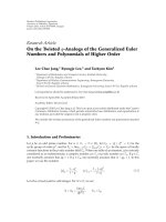
Figure 1: δx for α β 1 a and for α 5, β 0.5 b.
The approximation for u is a collocation function
p
t
: p
i
t
,t∈
τ
i
,τ
i1
,i 0, ,N − 1, 3.4
where we require p ∈ C
q−1
0, 1 in case that the order of the underlying differential equation
is q. Here, p
i
are polynomials of maximal degree m − 1 q which satisfy the system 3.2a at
m inner collocation points
t
i,j
τ
i
ρ
j
τ
i1
− τ
i
,i 0, ,N − 1,j 1, ,m
, 0 <ρ
1
< ···<ρ
m
< 1, 3.5
and the associated boundary conditions 3.2b.
Classical theory, compare 18, predicts that the convergence order for the global error
of the method is at least Oh
m
, where h is the maximal stepsize, h : max
i
τ
i1
− τ
i
. To
increase efficiency, an adaptive mesh selection strategy based on an a posteriori estimate for
the global error of the collocation solution is utilized. A more detailed description of the
numerical approach can be found in 4.
The code bvpsuite also allows to follow a path in the parameter-solution space. This
means that in the following problem setting, parameter ϑ is unknown:
F
t, u
4
t
,u
3
t
,u
t
,u
t
,u
t
,ϑ
0, 0 ≤ t ≤ 1, 3.6a
b
u
3
0
,u
0
,u
0
,u
0
,u
3
1
,u
1
,u
1
,u
1
0,ϑ λ, 3.6b
where λ is given. The path following strategy can also cope with turning points in the path.
The theoretical justification for the path following strategy implemented in bvpsuite has
been given in 19.
We first study the boundary problem 1.9a-1.9b. Positive solutions of problem
1.5a-1.5b will be discussed in Section 3.4.
24 Advances in Difference Equations
The above analytical discussion indicates that depending on the values of α, β, λ,the
problem has one or more positive solutions, a pseudo dead core solution or a dead core
solution. All numerical approximations have been calculated on a fixed mesh with N 500
subintervals and collocation degree m 4. Figure 1 shows δx for our choice of parameters
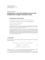
used in the following sections. Here, δ is given by 2.81.
3.1. Positive Solutions
For λ ∈ 0,δ0, δ04/93/3α 4β
3/2
, there exist a unique positive solution. This
solution was found numerically by using the original problem formulation 1.9a-1.9b. For
α β 1weobtainδ0 ≈ 0.12469. In Figure 2 we display the numerical solution, the error
estimate and the residual for λ 0.05. The residual rt is calculated by substituting the
numerical solution pt into the differential equation,
r
t
: p
t
−
λ
p
t
.
3.7
Due to the very small size of the error estimate and residual, it is obvious that the
numerical approximation is very accurate. According to the analytical results, a solution to
the problem satisfies |u0 −x
0
u1| 0 where x
0
is a root of δx − λ 0. Here, we have x
0
0.972608 and |u0 − x
0
u1| 6.410
−8
which again shows the high quality of the numerical
solution. In Figure 3 we depict the results for the parameter α 5, β 0.5andλ 0.02 <
δ0 ≈ 0.03294. For this choice of parameters x
0
0.877692 and |u0 − x
0
u1| 3.510
−8
.
For λ δ04/93/3α4β
3/2
there exists a unique positive solution. To compute
its numerical approximation, we rewrite the problem 1.9a-1.9b and consider
u
t
u
t
λ
4
9
3
3α 4β
3/2
,t∈
0, 1
,
u
0
0,αu
1
βu
1
1,α>0,β>0.
3.8
The numerical results related to parameter sets α 1, β 1, and α 5, β 0.5areshownin
Figure 4 and Figure 5, respectively.
Again, the error estimate and the residual are both very small and x
0
0.919315, so
|u0 − x
0
u1| 3.510
−7
. Moreover, for the second set of parameters, x
0
0.783283 and
|u0 − x
0
u1| 1.710
−8
.
For λ ∈ δ0,M with M max{δx :0≤ x ≤ 1} there exist two positive solutions.
These two different solutions for a fixed value of λ can be characterized via the roots x
1,2
of
δx − λ 0forx ∈ 0, 1. The choice of parameters remains the same. For α 1, β 1
and λ 0.15 the solution corresponding to x
1
≈ 0.009159 is shown in Figure 6.Thesolution
corresponding to x
2
≈ 0.896054 is depicted in Figure 7. Note that for these values of α and β
we have M ≈ 0.28049.
Advances in Difference Equations 25
0.925
0.93
0.935
0.94
0.945
ut
00.20.40.60.81
t
Solution
a
1.5
1.6
1.7
1.8
1.9
2
2.1
2.2
2.3
et
00.20.40.60.81
t
Error estimate
×10
−12
b
10
−12
rt
00.20.40.60.81
t
Residual
c
Figure 2: Problem 1.9a-1.9b: The numerical solution, the error estimate, and the residual for α 1, β 1
and λ 0.05.
0.175
0.18
0.185
0.19
0.195
ut
00.20.40.60.81
t
Solution
a
0.4
0.6
0.8
1
1.2
1.4
1.6
1.8
et
00.20.40.60.81
t
Error estimate
×10
−13
b
10
−14
10
−13
rt
00.20.40.60.81
t
Residual
c
Figure 3: Problem 1.9a-1.9b: The numerical solution, the error estimate, and the residual for α 5,
β 0.5andλ 0.02.
0.8
0.81
0.82
0.83
0.84
0.85
0.86
ut
00.20.40.60.81
t
Solution
a
1.5
1.6
1.7
1.8
1.9
2
2.1
2.2
et
00.20.40.60.81
t
Error estimate
×10
−11
b
10
−11
rt
00.20.40.60.81
t
Residual
c
Figure 4: Problem 3.8: The numerical solution, the error estimate, and the residual for α 1, β 1and
λ 4/93/3α 4β
3/2
.
0.155
0.16
0.165
0.17
0.175
0.18
0.185
0.19
ut
00.20.40.60.81
t
Solution
a
0.4
0.6
0.8
1
1.2
1.4
1.6
1.8
2
et
00.20.40.60.81
t
Error estimate
×10
−12
b
10
−13
10
−12
rt
00.20.40.60.81
t
Residual
c
Figure 5: Problem 3.8: The numerical solution, the error estimate, and the residual for α 5, β 0.5and
λ 4/93/3α 4β
3/2
.