Báo cáo sinh học: " Research Article New Existence Results for Higher-Order Nonlinear Fractional Differential Equation with Integral Boundary Conditions" pdf
Bạn đang xem bản rút gọn của tài liệu. Xem và tải ngay bản đầy đủ của tài liệu tại đây (691.72 KB, 20 trang )
Hindawi Publishing Corporation
Boundary Value Problems
Volume 2011, Article ID 720702, 20 pages
doi:10.1155/2011/720702
Research Article
New Existence Results for Higher-Order
Nonlinear Fractional Differential Equation with
Integral Boundary Conditions
Meiqiang Feng,
1
Xuemei Zhang,
2, 3
and WeiGao Ge
3
1
School of Applied Science, Beijing Information Science & Technology University, Beijing 100192, China
2
Department of Mathematics and Physics, North China E lectric Power University, Beijing 102206, China
3
Department of Mathematics, Beijing Institute of Technology, Beijing 100081, China
Correspondence should be addressed to Meiqiang Feng,
Received 16 March 2010; Revised 24 May 2010; Accepted 5 July 2010
Academic Editor: Feliz Manuel Minh
´
os
Copyright q 2011 Meiqiang Feng et al. This is an open access article distributed under the Creative
Commons Attribution License, which permits unrestricted use, distribution, and reproduction in
any medium, provided the original work is properly cited.
This paper investigates the existence and multiplicity of positive solutions for a class of higher-
order nonlinear fractional differential equations with integral boundary conditions. The results
are established by converting the problem into an equivalent integral equation and applying
Krasnoselskii’s fixed-point theorem in cones. The nonexistence of positive solutions is also studied.
1. Introduction
Fractional differential equations arise in many engineering and scientific disciplines as
the mathematical modelling of systems and processes in the fields of physics, chemistry,
aerodynamics, electrodynamics of complex medium, polymer rheology, Bode’s analysis of
feedback amplifiers, capacitor theory, electrical circuits, electron-analytical chemistry, biology,
control theory, fitting of experimental data, and so forth, and involves derivatives of fractional
order. Fractional derivatives provide an excellent tool for the description of memory and
hereditary properties of various materials and processes. This is the main advantage of
fractional differential equations in comparison with classical integer-order models. An
excellent account in the study of fractional differential equations can be found in 1–5. For
the basic theory and recent development of the subject, we refer a text by Lakshmikantham
6. For more details and examples, see 7–23 and the references therein. However, the theory
of boundary value problems for nonlinear fractional differential equations is still in the initial
stages and many aspects of this theory need to be explored.
2 Boundary Value Problems
In 23, Zhang used a fixed-point theorem for the mixed monotone operator to show
the existence of positive solutions to the following singular fractional differential equation.
D
α
0
u
t
q
t
f
t, x
t
,x
t
, ,x
n−2
t
0, 0 <t<1, 1.1
subject to the boundary conditions
u
0
u
0
u
0
··· u
n−2
0
u
n−1
1
0,
1.2
where D
α
0
is the standard Rimann-Liouville fractional derivative of order n−1 <α≤ n, n ≥ 2,
the nonlinearity f may be singular at u 0,u
0, ,u
n−2
0, and function qt may be
singular at t 0. The author derived the corresponding Green’s function named by fractional
Green’s function and obtained some properties as follows.
Proposition 1.1. Green’s function Gt, s satisfies the following conditions:
i Gt, s ≥ 0,Gt, s ≤ t
α−n2
/Γα − n 2,Gt, s ≤ Gs, s for all 0 ≤ t, s ≤ 1;
ii there exists a positive function ρ ∈ C0, 1 such that
min
γ≤t≤δ
G
t, s
≥ ρ
s
G
s, s
,s∈
0, 1
,
1.3
where 0 <γ<δ<1 and
ρ
s
⎧
⎪
⎪
⎪
⎪
⎨
⎪
⎪
⎪
⎪
⎩
δ
1 − s
α−n1
−
δ − s
α−n1
s
1 − s
α−n1
,s∈
0,r
,
γ
s
α−n1
,s∈
r, 1
,
1.4
here γ<r<δ.
It is well known that the cone theoretic techniques play a very important role in
applying Green’s function in the study of solutions to boundary value problems. In 23,the
author cannot acquire a positive constant taking instead of the role of positive function ρs
with n −1 <α≤ n, n ≥ 2in1.3. At the same time, we notice that many authors obtained the
similar properties to that of 1.3, for example, see Bai 12, Bai and L ¨u 13, Jiang and Yuan
14,Lietal,15, Kaufmann and Mboumi 19, and references therein. Naturally, one wishes
to find whether there exists a positive constant ρ such that
min
γ≤t≤δ
G
t, s
≥ ρG
s, s
,s∈
0, 1
,
1.5
for the fractional order cases. In Section 2, we will deduce some new properties of Green’s
function.
Boundary Value Problems 3
Motivated by the above mentioned work, we study the following higher-order
singular boundary value problem of fractional differential equation.
D
α
0
x
t
g
t
f
t, x
t
0, 0 <t<1
x
0
x
0
··· x
n−2
0
0,
x
1
1
0
h
t
x
t
dt,
P
where D
α
0
is the standard Rimann-Liouville fractional derivative of order n − 1 <α≤ n,
n ≥ 3,g∈ C0, 1, 0, ∞ and g may be singular at t 0or/andatt 1, h ∈ L
1
0, 1 is
nonnegative, and f ∈ C0, 1 × 0, ∞, 0, ∞.
For the case of α n,
1
0
htxtdt axη, 0 <η<1, 0 <aη
n−1
< 1, the boundary
value problems P reduces to the problem studied by Eloe and Ahmad in 24.In24,the
authors used the Krasnosel’skii and Guo 25 fixed-point theorem to show the existence of
at least one positive solution if f is either superlinear or sublinear to problem P. For the
case of α n,
1
0
htxtdt Σ
m−2
i1
ξ
i
xη
i
,ξ
i
∈ 0, ∞,η
i
∈ 0, 1,i 1, 2, ,n − 2, the
boundary value problems P is related to a m-point boundary value problems of integer-
order differential equation. Under this case, a great deal of research has been devoted to
the existence of solutions for problem P, for example, see Pang et al. 26,YangandWei
27, Feng and Ge 28, and references therein. All of these results are based upon the fixed-
point index theory, the fixed-point theorems and the fixed-point theory in cone for strict set
contraction operator.
The organization of this paper is as follows. We will introduce some lemmas and
notations in the rest of this section. In Section 2, we present the expression and properties of
Green’s function associated with boundary value problem P .InSection 3, we discuss some
characteristics of the integral operator associated with the problem P and state a fixed-
point theorem in cones. In Section 4, we discuss the existence of at least one positive solution
of boundary value problem P .InSection 5, we will prove the existence of two or m positive
solutions, where m is an arbitrary natural number. In Section 6, we study the nonexistence of
positive solution of boundary value problem P.InSection 7, one example is also included
to illustrate the main results. Finally, conclusions in Section 8 close the paper.
The fractional differential equations related notations adopted in this paper can be
found, if not explained specifically, in almost all literature related to fractional differential
equations. The readers who are unfamiliar with this area can consult, for example, 1–6 for
details.
Definition 1.2 see
4. The integral
I
α
0
f
x
1
Γ
α
x
0
f
t
x − t
1−α
dt, x > 0,
1.6
where α>0, is called Riemann-Liouville fractional integral of order α.
4 Boundary Value Problems
G
1
(τ(s),s)
G
1
(s, s)
0.20.40.60.81
s
0.02
0.04
0.06
0.08
0.12
0.1
z
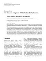
Figure 1: Graph of functions G
1
τs,s G
1
s, s for α 5/2.
Definition 1.3 see 4. For a function fx given in the interval 0, 1, the expression
D
α
0
f
x
1
Γ
n − α
d
dx
n
x
0
f
t
x − t
α−n1
dt,
1.7
where n α1, α denotes the integer part of number α, is called the Riemann-Liouville
fractional derivative of order α.
Lemma 1.4 see 13. Assume that u ∈ C0, 1 ∩L0, 1 with a fractional derivative of order α>0
that belongs to u ∈ C0, 1 ∩ L0, 1.Then
I
α
0
D
α
0
u
t
u
t
C
1
t
α−1
C
2
t
α−2
··· C
N
t
α−N
,
1.8
for some C
i
∈ R, i 1, 2, ,N,whereN is the smallest integer greater than or equal to α.
2. Expression and Properties of Green’s Function
In this section, we present the expression and properties of Green’s function associated with
boundary value problem P.
Lemma 2.1. Assume that
1
0
htt
α−1
dt
/
1. Then for any y ∈ C0, 1, the unique solution of
boundary value problem
D
α
0
x
t
y
t
0, 0 <t<1
x
0
x
0
x
n−2
0
0,
x
1
1
0
h
t
x
t
dt
2.1
Boundary Value Problems 5
τ(s)
0.20.40.60.81
0.4
0.5
0.6
0.7
0.8
0.9
Figure 2: Graph of function τs for α 5/2.
is given by
x
t
1
0
G
t, s
y
s
ds,
2.2
where
G
t, s
G
1
t, s
G
2
t, s
, 2.3
G
1
t, s
⎧
⎪
⎪
⎪
⎪
⎪
⎪
⎨
⎪
⎪
⎪
⎪
⎪
⎪
⎩
t
α−1
1 − s
α−1
− t − s
α−1
Γ
α
, 0 ≤ s ≤ t ≤ 1,
t
α−1
1 − s
α−1
Γ
α
, 0 ≤ t ≤ s ≤ 1,
2.4
G
2
t,s
t
α−1
1 −
1
0
h
t
t
α−1
dt
1
0
h
t
G
1
t, s
dt. 2.5
Proof . By Lemma 1.4, we can reduce the equation of problem 2.1 to an equivalent integral
equation
x
t
−I
α
0
y
t
c
1
t
α−1
c
2
t
α−2
··· c
n
t
α−n
−
1
Γ
α
t
0
t − s
α−1
y
s
ds c
1
t
α−1
c
2
t
α−2
··· c
n
t
α−n
.
2.6
By x00, there is c
n
0. Thus,
x
t
−I
α
0
y
t
c
1
t
α−1
c
2
t
α−2
··· c
n−1
t
α−n1
.
2.7
6 Boundary Value Problems
Differentiating 2.7, we have
x
t
−
α − 1
Γ
α
t
0
t − s
α−2
y
s
ds c
1
α − 1
t
α−2
··· c
n−1
α − n 1
t
α−n
.
2.8
By 2.8 and x
00, we have c
n−1
0. Similarly, we can obtain that c
2
c
3
··· c
n−2
0.
Then
x
t
−
1
Γ
α
t
0
t − s
α−1
y
s
ds c
1
t
α−1
.
2.9
By x1
1
0
htxtdt, we have
c
1
1
0
h
t
x
t
dt
1
Γ
α
1
0
1 − s
α−1
y
s
ds.
2.10
Therefore, the unique solution of BVP 2.1 is
x
t
−
1
Γ
α
t
0
t − s
α−1
y
s
ds t
α−1
1
0
h
t
x
t
dt
1
Γ
α
1
0
1 − s
α−1
y
s
ds
1
0
G
1
t, s
y
s
ds t
α−1
1
0
h
t
x
t
dt,
2.11
where G
1
t, s is defined by 2.4.
From 2.11, we have
1
0
h
t
x
t
dt
1
0
h
t
1
0
G
1
t, s
y
s
ds dt
1
0
h
t
t
α−1
dt
1
0
h
t
x
t
dt.
2.12
It follows that
1
0
h
t
x
t
dt
1
1 −
1
0
h
t
t
α−1
dt
1
0
h
t
1
0
G
1
t, s
y
s
ds dt.
2.13
Substituting 2.13 into 2.11,weobtain
x
t
1
0
G
1
t, s
y
s
ds
t
α−1
1 −
1
0
h
t
t
α−1
dt
1
0
h
t
1
0
G
1
t, s
y
s
ds dt
1
0
G
1
t, s
y
s
ds
1
0
G
2
t, s
y
s
ds
1
0
G
t, s
y
s
ds,
2.14
Boundary Value Problems 7
where Gt, s,G
1
t, s, and G
2
t, s are defined by 2.3, 2.4,and2.5, respectively. The
proof is complete.
From 2.3, 2.4,and2.5, we can prove that Gt, s,G
1
t, s, and G
2
t, s have the
following properties.
Proposition 2.2. The function G
1
t, s defined by 2.4 satisfies
i G
1
t, s ≥ 0 is continuous for all t, s ∈ 0, 1,G
1
t, s > 0, for all t, s ∈ 0, 1;
ii for all t ∈ 0, 1,s∈ 0, 1, one has
G
1
t, s
≤ G
1
τ
s
,s
τs
α−1
1 − s
α−1
− τs − s
α−1
Γ
α
,
2.15
where
τ
s
s
1 − 1 − s
α−1/α−2
.
2.16
Proof. i It is obvious that G
1
t, s is continuous on 0, 1 × 0, 1 and G
1
t, s ≥ 0 when s ≥ t.
For 0 ≤ s<t≤ 1, we have
t
α−1
1 − s
α−1
− t − s
α−1
1 − s
α−1
t
α−1
−
t − s
1 − s
α−1
≥ 0. 2.17
So, by 2.4, we have
G
1
t, s
≥ 0, ∀t, s ∈
0, 1
. 2.18
Similarly, for t, s ∈ 0, 1, we have G
1
t, s > 0.
ii Since n − 1 <α≤ n, n ≥ 3, it is clear that G
1
t, s is increasing with respect to t for
0 ≤ t ≤ s ≤ 1.
On the other hand, from the definition of G
1
t, s, for given s ∈ 0, 1,s < t ≤ 1, we
have
∂G
1
t, s
∂t
α − 1
Γ
α
t
α−2
1 − s
α−1
−
t − s
α−2
.
2.19
Let
∂G
1
t, s
∂t
0.
2.20
Then, we have
t
α−2
1 − s
α−1
t − s
α−2
,
2.21
8 Boundary Value Problems
and so,
1 − s
α−1
1 −
s
t
α−2
.
2.22
Noticing α>2, from 2.22, we have
t
s
1 − 1 − s
α−1/α−2
: τ
s
.
2.23
Then, for given s ∈ 0, 1, we have G
1
t, s arrives at maximum at τs,s when s<t.
This together with the fact that G
1
t, s is increasing on s ≥ t,weobtainthat2.15 holds.
Remark 2.3. From Figure 1, we can see that G
1
s, s ≤ G
1
τs,s for α>2. If 1 <α≤ 2, then
G
1
t, s
≤ G
1
s, s
s
α−1
1 − s
α−1
Γ
α
.
2.24
Remark 2.4. From Figure 2, we can see that τs is increasing with respect to s.
Remark 2.5. From Figure 3, we can see that G
1
τs,s > 0fors ∈ J
θ
θ, 1 − θ, where
θ ∈ 0, 1/2.
Remark 2.6. Let
G
1
τs,sτs
α−1
1 − s
α−1
− τs − s
α−1
.From2.15,fors ∈ 0, 1,we
have
d
G
1
τ
s
,s
ds
−
α − 1
1 − s
α−2
τs
α−1
−
α − 1
τ
s
− s
α−2
×
⎛
⎜
⎝
−1
1
1 − 1 − s
α−1/α−2
−
α − 1
1 − s
−1α−1/α−2
s
α − 2
1 −
1 − s
α−1/α−2
2
⎞
⎟
⎠
α − 1
1 − s
α−1
τs
α−2
×
⎛
⎜
⎝
1
1 − 1 − s
α−1/α−2
−
α − 1
1 − s
α−1/α−2
s
α − 2
1 −
1 − s
α−1/α−2
2
⎞
⎟
⎠
.
2.25
Remark 2.7. From 2.25, we have
lim
s →0
dG
1
τ
s
,s
ds
α − 1
−
α − 2
α − 1
α−1
α − 2
α − 1
α−2
: f
α
. 2.26
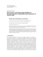
Remark 2.8. From Figure 4,itiseasytoobtainthatfα is decreasing with respect to α,and
lim
α →2
f
α
1, lim
α →∞
f
α
1
e
.
2.27
Boundary Value Problems 9
Proposition 2.9. There exists γ>0 such that
min
t∈
θ,1−θ
G
1
t, s
≥ γG
1
τ
s
,s
, ∀s ∈
0, 1
.
2.28
Proof. For t ∈ J
θ
, we divide the proof into the following three cases for s ∈ 0, 1.
Case 1. If s ∈ J
θ
, then from i of Proposition 2.2 and Remark 2.5, we have
G
1
t, s
> 0,G
1
τ
s
,s
> 0, ∀t, s ∈ J
θ
. 2.29
It is obvious that G
1
t, s and G
1
τs,s are bounded on J
θ
. So, there exists a constant γ
1
> 0
such that
G
1
t, s
≥ γ
1
G
1
τ
s
,s
, ∀t, s ∈ J
θ
. 2.30
Case 2. If s ∈ 1 − θ, 1, then from 2.4, we have
G
1
t, s
t
α−1
1 − s
α−1
Γ
α
.
2.31
On the other hand, from the definition of τs,weobtainthatτs takes its maximum
1ats 1. So
G
1
τ
s
,s
τ
s
α−1
1 − s
α−1
−
τ
s
− s
α−1
Γ
α
≤
τ
s
α−1
1 − s
α−1
Γ
α
τ
s
α−1
t
α−1
1 − s
α−1
t
α−1
Γ
α
≤
1
θ
α−1
G
1
t, s
.
2.32
Therefore, G
1
t, s ≥ θ
α−1
G
1
τs,s. Letting θ
α−1
γ
2
, we have
G
1
t, s
≥ γ
2
G
1
τ
s
,s
. 2.33
Case 3. If s ∈ 0,θ,fromi of Proposition 2.2, it is clear that
G
1
t, s
> 0,G
1
τ
s
,s
> 0, ∀t ∈ J
θ
,s∈
0,θ
. 2.34
10 Boundary Value Problems
In view of Remarks 2.6–2.8, we have
lim
s →0
G
1
t, s
G
1
τ
s
,s
lim
s →0
t
α−1
1 − s
α−1
− t − s
α−1
τs
α−1
1 − s
α−1
− τs − s
α−1
lim
s →0
−
α − 1
t
α−1
1 − s
α−2
−
α − 1
t − s
α−2
dG
1
τ
s
,s
/ds
> 0.
2.35
From 2.35, there exists a constant γ
3
such that
G
1
t, s
≥ γ
3
G
1
τ
s
,s
. 2.36
Letting γ min{γ
1
,γ
2
,γ
3
} and using 2.30, 2.33,and2.36, it follows that 2.28 holds. This
completes the proof.
Let
μ
1
0
h
t
t
α−1
dt.
2.37
Proposition 2.10. If μ ∈ 0, 1, then one has
i G
2
t, s ≥ 0 is continuous for all t, s ∈ 0, 1,G
2
t, s > 0, for all t, s ∈ 0, 1;
ii G
2
t, s ≤ 1/1 − μ
1
0
htG
1
t, sdt, for all t ∈ 0, 1,s∈ 0, 1.
Proof. Using the properties of G
1
t, s, definition of G
2
t, s, it can easily be shown that i and
ii hold.
Theorem 2.11. If μ ∈ 0, 1, the function Gt, s defined by 2.3 satisfies
i Gt, s ≥ 0 is continuous for all t, s ∈ 0, 1,Gt, s > 0, for all t, s ∈ 0, 1;
ii Gt, s ≤ Gs for each t, s ∈ 0, 1, and
min
t∈θ,1−θ
G
t, s
≥ γ
∗
G
s
, ∀s ∈
0, 1
,
2.38
where
γ
∗
min
γ,θ
α−1
,G
s
G
1
τ
s
,s
G
2
1,s
, 2.39
τs is defined by 2.16, γ is defined in Proposition 2.9.
Boundary Value Problems 11
Proof. i From Propositions 2.2 and 2.10,weobtainthatGt, s ≥ 0 is continuous for all
t, s ∈ 0, 1,andGt, s > 0, for all t, s ∈ 0, 1.
ii From ii of Proposition 2.2 and ii of Proposition 2.10, we have that Gt, s ≤ Gs
for each t, s ∈ 0, 1.
Now, we show that 2.38 holds.
In fact, from Proposition 2.9, we have
min
t∈J
θ
G
t, s
≥ γG
1
τ
s
,s
θ
α−1
1 − μ
1
0
h
t
G
1
t, s
dt
≥ γ
∗
G
1
τ
s
,s
1
1 − μ
1
0
h
t
G
1
t, s
dt
γ
∗
G
s
, ∀s ∈
0, 1
.
2.40
Then the proof of Theorem 2.11 is completed.
Remark 2.12. From the definition of γ
∗
, it is clear that 0 <γ
∗
< 1.
3. Preliminaries
Let J 0, 1 and E C0, 1 denote a real Banach space with the norm ·defined by
x max
0≤t≤1
|xt|. Let
K
x ∈ E : x ≥ 0, min
t∈J
θ
x
t
≥ γ
∗
x
,
K
r
{
x ∈ K : x≤r
}
,∂K
r
{
x ∈ K : x r
}
.
3.1
To prove the existence of positive solutions for the boundary value problem P,we
need the following assumptions:
H
1
g ∈ C0, 1, 0, ∞,gt
✚
≡ 0 on any subinterval of 0,1 and 0 <
1
0
Gsgsds <
∞, where Gs is defined in Theorem 2.11;
H
2
f ∈ C0, 1 × 0, ∞, 0, ∞ and ft, 00 uniformly with respect to t on 0, 1;
H
3
μ ∈ 0, 1, where μ is defined by 2.37.
From condition H
1
,itisnotdifficult to see that g may be singular at t 0or/andat
t 1, that is, lim
t →0
gt∞ or/and lim
t →1
−
gt∞.
Define T : K → K by
Tx
t
1
0
G
t, s
g
s
f
s, x
s
ds,
3.2
where Gt, s is defined by 2.3.
12 Boundary Value Problems
Lemma 3.1. Let H
1
–H
3
hold. Then boundary value problems P has a solution x if and only if
x is a fixed point of T.
Proof. From Lemma 2.1, we can prove the result of this lemma.
Lemma 3.2. Let H
1
–H
3
hold. Then TK ⊂ K and T : K → K is completely c ontinuous.
Proof. For any x ∈ K,by3.2, we can obtain that Tx ≥ 0. On the other hand, by ii of
Theorem 2.11, we have
Tx
t
≤
1
0
G
s
g
s
f
s, x
s
ds.
3.3
Similarly, by 2.38,weobtain
Tx
t
≥ γ
∗
1
0
G
s
g
s
f
s, x
s
ds
γ
∗
Tx
,t∈ J
θ
.
3.4
So, Tx ∈ K and hence TK ⊂ K. Next by similar proof of Lemma 3.1in13 and Ascoli-
Arzela theorem one can prove T : K → K is completely continuous. So it is omitted.
To obtain positive solutions of boundary value problem P, the following fixed-point
theorem in cones is fundamental which can be found in 25, page 94.
Lemma 3.3 Fixed-point theorem of cone expansion and compression of norm type. Let P be
a cone of real Banach space E, and let Ω
1
and Ω
2
be two bounded open sets in E such that 0 ∈ Ω
1
and
Ω
1
⊂ Ω
2
. Let operator A : P ∩Ω
2
\Ω
1
→ P be completely continuous. Suppose that one of the two
conditions
i Ax≤x, for all x ∈ P ∩ ∂Ω
1
and Ax≥x, for all x ∈ P ∩ ∂Ω
2
or
ii Ax≥x, for all x ∈ P ∩ ∂Ω
1
, and Ax≤x, for all x ∈ P ∩ ∂Ω
2
is satisfied. Then A has at least one fixed point in P ∩ Ω
2
\ Ω
1
.
4. Existence of Positive Solution
In this section, we impose growth conditions on f which allow us to apply Lemma 3.3 to
establish the existence of one positive solution of boundary value problem P, and we begin
by introducing some notations:
f
β
lim sup
x →β
max
t∈0,1
f
t, x
x
,f
β
lim inf
x →β
min
t∈0,1
f
t, x
x
,
4.1
Boundary Value Problems 13
where β denotes 0 or ∞, and
σ
1
0
G
s
g
s
ds.
4.2
Theorem 4.1. Assume that H
1
–H
3
hold. In addition, one supposes that one of the following
conditions is satisfied:
C
1
f
0
> 1/
1−θ
θ
Gsgsdsγ
∗
2
and f
∞
< 1/σ (particularly, f
0
∞ and f
∞
0).
C
2
there exist two constants r
2
,R
2
with 0 <r
2
≤ R
2
such that ft, · is nondecreasing on
0,R
2
for all t ∈ 0, 1, and ft, γ
∗
r
2
≥ r
2
/γ
∗
1−θ
θ
Gsgsds, and ft, R
2
≤ R
2
/σ for all t ∈ 0, 1.
Then boundary value problem P has at least one positive solution.
Proof. Let T be cone preserving completely continuous that is defined by 3.2.
Case 1. The condition C
1
holds. Considering f
0
> 1/
1−θ
θ
Gsgsdsγ
∗
2
, there exists
r
1
> 0 such that ft, x ≥ f
0
− ε
1
x,fort ∈ 0, 1,x∈ 0,r
1
, where ε
1
> 0satisfies
1−θ
θ
Gsgsdsγ
∗
2
f
0
− ε
1
≥ 1. Then, for t ∈ 0, 1,x∈ ∂K
r
1
, we have
Tx
t
1
0
G
t, s
g
s
f
s, x
s
ds
≥ γ
∗
1
0
G
s
g
s
f
s, x
s
ds
≥ γ
∗
1
0
G
s
g
s
f
0
− ε
1
x
s
ds
≥
γ
∗
2
f
0
− ε
1
1−θ
θ
G
s
g
s
ds
x
≥
x
,
4.3
that is, x ∈ ∂K
r
1
imply that
Tx
≥
x
. 4.4
Next, turning to f
∞
< 1/σ, there exists R
1
> 0 such that
f
t, x
≤
f
∞
ε
2
x, for t ∈
0, 1
,x∈
R
1
, ∞
, 4.5
where ε
2
> 0satisfiesσf
∞
ε
2
≤ 1.
Set
M max
0≤x≤R
1
,t∈
0,1
f
t, x
,
4.6
then ft, x ≤ M f
∞
ε
2
x.
14 Boundary Value Problems
Chose R
1
> max{r
1
, R
1
,Mσ1 − σf
∞
ε
2
−1
}. Then, for x ∈ ∂K
R
1
, we have
Tx
t
1
0
G
t, s
g
s
f
s, x
s
ds
≤
1
0
G
s
g
s
f
s, x
s
ds
≤
1
0
G
s
g
s
M
f
∞
ε
2
x
s
ds
≤ M
1
0
G
s
g
s
ds
f
∞
ε
2
1
0
G
s
g
s
ds
x
<R
1
− σ
f
∞
ε
2
R
1
f
∞
ε
2
σ
x
R
1
,
4.7
that is, x ∈ ∂K
R
1
imply that
Tx
<
x
. 4.8
Case 2. The Condition C
2
satisfies. For x ∈ K,from3.1 we obtain that min
t∈J
θ
xt ≥ γ
∗
x.
Therefore, for x ∈ ∂K
r
2
, we have xt ≥ γ
∗
x γ
∗
r
2
for t ∈ J
θ
, this together with C
2
,we
have
Tx
t
1
0
G
t, s
g
s
f
s, x
s
ds
≥ γ
∗
1−θ
θ
G
s
g
s
f
s, γ
∗
r
2
ds
≥ γ
∗
1
γ
∗
1−θ
θ
G
s
g
s
ds
r
2
1−θ
θ
G
s
g
s
ds
r
2
x
,
4.9
that is, x ∈ ∂K
r
2
imply that
Tx
≥
x
. 4.10
Boundary Value Problems 15
On the other hand, for x ∈ ∂K
R
2
, we have that xt ≤ R
2
for t ∈ 0, 1, this together with C
2
,
we have
Tx
t
1
0
G
t, s
g
s
f
s, x
s
ds
≤
1
0
G
s
g
s
f
s, x
s
ds
≤
R
2
σ
1
0
G
s
g
s
ds
R
2
,
4.11
that is, x ∈ ∂K
R
2
imply that
Tx
≤
x
. 4.12
Applying Lemma 3.3 to 4.4 and 4.8,or4.10 and 4.12, yields that T has a fixed
point x
∗
∈ K
r,R
or x
∗
∈ K
r
i
,R
i
i 1, 2 with x
∗
t ≥ γ
∗
x
∗
> 0,t ∈ 0, 1. Thus it follows that
boundary value problems P has a positive solution x
∗
, and the theorem is proved.
Theorem 4.2. Assume that H
1
–H
3
hold. In addition, one supposes that the following condition
is satisfied:
C
3
f
0
< 1/σ and f
∞
> 1/
1−θ
θ
Gsgsdsγ
∗
2
(particularly, f
0
0 and f
∞
∞).
Then boundary value problem P has at least one positive solution.
5. The Existence of Multiple Positive Solutions
Now we discuss the multiplicity of positive solutions for boundary value problem P.We
obtain the following existence results.
Theorem 5.1. Assume H
1
–H
3
, and the following two conditions:
C
4
f
0
> 1/
1−θ
θ
Gsgsdsγ
∗
2
and f
∞
> 1/
1−θ
θ
Gsgsdsγ
∗
2
(particularly, f
0
f
∞
∞);
C
5
there exists b>0 such that max
t∈0,1,x∈∂K
b
ft, x <b/σ.
Then boundary value problem P has at least two positive solutions x
∗
t,x
∗∗
t, which satisfy
0 <
x
∗∗
<b<
x
∗
. 5.1
Proof. We consider condition C
4
. Choose r, R with 0 <r<b<R.
If f
0
> 1/
1−θ
θ
Gsgsdsγ
∗
2
, then by the proof of 4.4, we have
Tx
≥
x
, for x ∈ ∂K
r
. 5.2
16 Boundary Value Problems
If f
∞
> 1/
1−θ
θ
Gsgsdsγ
∗
2
, then similar to the proof of 4.4, we have
Tx
≥
x
, for x ∈ ∂K
R
. 5.3
On the other hand, by C
5
,forx ∈ ∂K
b
, we have
Tx
t
1
0
G
t, s
g
s
f
s, x
s
ds
≤
1
0
G
s
g
s
f
s, x
s
ds
≤
b
σ
1
0
G
s
g
s
ds
b.
5.4
By 5.4, we have
Tx
<b
x
. 5.5
Applying Lemma 3.3 to 5.2, 5.3,and5.5 yields that T has a fixed point x
∗∗
∈ K
r,b
,
and a fixed point x
∗
∈ K
b,R
. Thus it follows that boundary value problem P has at least two
positive solutions x
∗
and x
∗∗
. Noticing 5.5 , we have x
∗
/
b and x
∗∗
/
b. Therefore 5.1
holds, and the proof is complete.
Theorem 5.2. Assume H
1
–H
3
, and the following two conditions:
C
6
f
0
< 1/σ and f
∞
< 1/σ;
C
7
there exists B>0 such that min
t∈J
θ
,x∈∂K
B
ft, x >B/
1−θ
θ
Gsgsdsγ
∗
.
Then boundary value problem P has at least two positive solutions x
∗
t,x
∗∗
t, which satisfy
0 < x
∗∗
<B<x
∗
. 5.6
Theorem 5.3. Assume that H
1
, H
2
, and H
3
hold. If there exist 2m positive numbers
d
k
,D
k
,k 1, 2, ,m with d
1
<γ
∗
D
1
<D
1
<d
2
<γ
∗
D
2
<D
2
< ··· <d
m
<γ
∗
D
m
<D
m
such that
C
8
ft, x ≥ 1/
1−θ
θ
Gsgsdsγ
∗
d
k
for t, x ∈ 0, 1 × γ
∗
d
k
,d
k
and ft, x ≤ σ
−1
D
k
for t, x ∈ 0, 1 × γ
∗
D
k
,D
k
,k 1, 2, ,m.
Then boundary value problem P has at least m positive solutions x
k
satisfying d
k
≤x
k
≤D
k
,k
1, 2, ,m.
Boundary Value Problems 17
Theorem 5.4. Assume that H
1
, H
2
, and H
3
hold. If there exist 2m positive numbers
d
k
,D
k
,k 1, 2, ,mwith d
1
<D
1
<d
2
<D
2
< ···<d
m
<D
m
such that
C
9
ft, · is nondecreasing on 0,D
m
for all t ∈ 0, 1;
C
10
ft, γ
∗
d
k
≥ d
2
/
1−θ
θ
Gsgsdsγ
∗
, and ft, D
k
≤ σ
−1
D
k
,k 1, 2, ,m.
Then boundary value problem P has at least m positive solutions x
k
satisfying d
k
≤x
k
≤D
k
,k
1, 2, ,m.
6. The Nonexistence of Positive Solution
Our last results corresponds to the case when boundary value problem P has no positive
solution.
Theorem 6.1. Assume H
1
–H
3
and ft, x <σ
−1
x, for all t ∈ J, x > 0, then boundary value
problem P has no positive solution.
Proof. Assume to the contrary that xt is a positive solution of the boundary value problem
P. Then,x ∈ K, xt > 0for t ∈ 0, 1,and
x max
t∈J
|
x
t
|
1
0
G
t, s
g
s
f
s, x
s
ds
≤
1
0
G
s
g
s
f
s, x
s
ds
<
1
0
G
s
g
s
1
σ
x
ds
1
σ
1
0
G
s
g
s
ds
x
x
,
6.1
which is a contradiction, and complete the proof.
Similarly, we have the following results.
Theorem 6.2. Assume H
1
−H
3
and ft, x > 1/
1−θ
θ
Gsgsdsγ
∗
2
x, for all x>0,t∈
J, then boundary value problem P has no positive solution.
7. Example
To illustrate how our main results can be used in practice we present an example.
18 Boundary Value Problems
G
1
(τ(s),s)
0.35 0.45 0.5
0.55
0.60.65
0.088
0.092
0.094
0.096
0.098
0.09
Figure 3: Graph of function G
1
τs,s for θ 1/3, α 5/2.
Example 7.1. Consider the following boundary value problem of nonlinear fractional
differential equations:
−D
5/2
0
x
1
√
t
t x
1/3
tanh x x
1/3
,
x
0
0,x
0
0,
x
1
1
0
1
6
|
t − 1/2
|
2/3
x
t
dt,
7.1
where
α
5
2
,g
t
1
√
t
,h
t
1
6
|
t − 1/2
|
2/3
,
f
t, x
t x
1/3
tanh x x
1/3
.
7.2
It is easy to see that H
1
–H
3
hold. By simple computation, we have
f
0
∞,f
∞
0, 7.3
thus it follows that problem 7.1 has a positive solution by C
1
.
8. Conclusions
In this paper, by using the famous Guo-Krasnoselskii fixed-point theorem, we have
investigated the existence and multiplicity of positive solutions for a class of higher-order
nonlinear fractional differential equations with integral boundary conditions and obtained
some easily verifiable sufficient criteria. The interesting point is that we obtain some new
positive properties of Green’s function, which significantly extend and improve many known
results for fractional order cases, for example, see 12–15, 19. The methodology which we
employed in studying the boundary value problems of integer-order differential equation
Boundary Value Problems 19
f(α)
200 400 600 800 1000
0.37
0.38
0.39
0.41
Figure 4: Graph of function fα for α>2.
in 28 can be modified to establish similar sufficient criteria for higher-order nonlinear
fractional differential equations. It is worth mentioning that there are still many problems
that remain open in this vital field except for the results obtained in this paper: for example,
whether or not we can obtain the similar results of fractional differential equations with p-
Laplace operator by employing the same technique of this paper, and whether or not our
concise criteria can guarantee the existence of positive solutions for higher-order nonlinear
fractional differential equations with impulses. More efforts are still needed in the future.
Acknowledgments
The authors thank the referee for his/her careful reading of the manuscript and useful
suggestions. These have greatly improved this paper. This work is sponsored by the Funding
Project for Academic Human Resources Development in Institutions of Higher Learning
Under the Jurisdiction of Beijing Municipality PHR201008430, the Scientific Research
Common Program of Beijing Municipal Commission of Education KM201010772018,
the 2010 level of scientific research of improving project 5028123900, the Graduate
Technology Innovation Project 5028211000 and Beijing Municipal Education Commission
71D0911003.
References
1 K. S. Miller and B. Ross, An Introduction to the Fractional Calculus and Fractional Differential Equations,
A Wiley-Interscience Publication, John Wiley & Sons, New York, NY, USA, 1993.
2 K. B. Oldham and J. Spanier, The Fractional Calculus: Theory and Applications of Differentiation and
Integration to Arbitrary Order, vol. 11 of Mathematics in Science and Engineering, Academic Press,
London, UK, 1974.
3 I. Podlubny, Fractional Differential Equations: An Introduction to Fractional Derivatives, Fractional
Differential Equations, to Methods of Their Solution and Some of Their Applications, vol. 198 of Mathematics
in Science and Engineering, Academic Press, San Diego, Calif, USA, 1999.
4 S. G. Samko, A. A. Kilbas, and O. I. Marichev, Fractional Integrals and Derivatives: Theory and
Applications, Gordon and Breach, Yverdon, Switzerland, 1993.
5 A. A. Kilbas, H. M. Srivastava, and J. J. Trujillo, Theory and Applications of Fractional Differential
Equations, vol. 204 of North-Holland Mathematics Studies, Elsevier, Amsterdam, The Netherlands, 2006.
6 V. Lakshmikantham, S. Leela, and J. Vasundhara Devi, Theory of Fractional Dynamic Systems,
Cambridge Academic, Cambridge, UK, 2009.
20 Boundary Value Problems
7 V. Lakshmikantham and A. S. Vatsala, “Basic theory of fractional differential equations,” Nonlinear
Analysis: Theory, Methods & Applications, vol. 69, no. 8, pp. 2677–2682, 2008.
8 V. Lakshmikantham, “Theory of f ractional functional differential equations,” Nonlinear Analysis:
Theory, Methods & Applications, vol. 69, no. 10, pp. 3337–3343, 2008.
9 V. Lakshmikantham and A. S. Vatsala, “General uniqueness and monotone iterative technique for
fractional differential equations,” Applied Mathematics Letters, vol. 21, no. 8, pp. 828–834, 2008.
10 B. Ahmad and J. J. Nieto, “Existence of solutions for nonlocal boundary value problems of higher-
order nonlinear fractional differential equations,” Abstract and Applied Analysis, vol. 2009, Article ID
494720, 9 pages, 2009.
11 B. Ahmad and J. J. Nieto, “Existence results for nonlinear boundary value problems of fractional
integrodifferential equations with integral boundary conditions,” Boundary Value Problems, vol. 2009,
Article ID 708576, 11 pages, 2009.
12 Z. Bai, “On positive solutions of a nonlocal fractional boundary value problem,” Nonlinear Analysis:
Theory, Methods & Applications, vol. 72, no. 2, pp. 916–924, 2010.
13 Z. Bai and H. L
¨
u, “Positive solutions for boundary value problem of nonlinear fractional differential
equation,” Journal of Mathematical Analysis and Applications, vol. 311, no. 2, pp. 495–505, 2005.
14 D. Jiang and C. Yuan, “The positive properties of the Green function for Dirichlet-type boundary
value problems of nonlinear fractional differential equations and its application,” Nonlinear Analysis:
Theory, Methods and Applications, vol. 72, no. 2, pp. 710–719, 2009.
15 C. F. Li, X. N. Luo, and Y. Zhou, “Existence of positive solutions of the boundary value problem for
nonlinear fractional differential equations,” Computers and Mathematics with Applications, vol. 59, no.
3, pp. 1363–1375, 2010.
16 M. Benchohra, S. Hamani, and S. K. Ntouyas, “Boundary value problems for differential equations
with fractional order and nonlocal conditions,” Nonlinear Analysis: Theory, Methods and Applications,
vol. 71, no. 7-8, pp. 2391–2396, 2009.
17 H. A. H. Salem, “On the nonlinear Hammerstein integral equations in Banach spaces and application
to the boundary value problem of fractional order,” Mathematical and Computer Modelling
, vol. 48, no.
7-8, pp. 1178–1190, 2008.
18 H. A. H. Salem, “On the fractional order m-point boundary value problem in reflexive Banach spaces
and weak topologies,” Journal of Computational and Applied Mathematics, vol. 224, no. 2, pp. 565–572,
2009.
19 E. R. Kaufmann and E. Mboumi, “Positive solutions of a boundary value problem for a nonlinear
fractional differential equation,” Electronic Journal of Qualitative Theory of Differential Equations, vol.
2008, no. 3, pp. 1–11, 2008.
20 S. Zhang, “Positive solutions for boundary-value problems of nonlinear fractional differential
equations,” Electronic Journal of Differential Equations, vol. 2006, pp. 1–12, 2006.
21 S. Zhang, “The existence of a positive solution for a nonlinear fractional differential equation,” Journal
of Mathematical Analysis and Applications, vol. 252, no. 2, pp. 804–812, 2000.
22 S. Zhang, “Existence of positive solution for some class of nonlinear fractional differential equations,”
Journal of Mathematical Analysis and Applications, vol. 278, no. 1, pp. 136–148, 2003.
23 S. Zhang, “Positive solutions to singular boundary value problem for nonlinear fractional differential
equation,” Computers and Mathematics with Applications, vol. 59, no. 3, pp. 1300–1309, 2010.
24 P. W. Eloe and B. Ahmad, “Positive solutions of a nonlinear nth order boundary value problem with
nonlocal conditions,” Applied Mathematics Letters, vol. 18, no. 5, pp. 521–527, 2005.
25 D. Guo, V. Lakshmikantham, and X. Liu, Nonlinear Integral Equations in Abstract Spaces, vol. 373 of
Mathematics and Its Applications, Kluwer Academic Publishers, Dordrecht, The Netherlands, 1996.
26 C. Pang, W. Dong, and Z. Wei, “Green’s function and positive solutions of nth order m-point boundary
value problem,” Applied Mathematics and Computation, vol. 182, no. 2, pp. 1231–1239, 2006.
27 J. Yang and Z. Wei, “Positive solutions of nth order m-point boundary value problem,” Applied
Mathematics and Computation, vol. 202, no. 2, pp. 715–720, 2008.
28 M. Feng and W. Ge, “Existence results for a class of nth order m-point boundary value problems in
Banach spaces,” Applied Mathematics Letters, vol. 22, no. 8, pp. 1303–1308, 2009.