Báo cáo sinh học: " Research Article Correlation-Based Amplitude Estimation of Coincident Partials in Monaural Musical Signals" ppt

Hindawi Publishing Corporation
EURASIP Journal on Audio, Speech, and Music Processing
Volume 2010, Article ID 523791, 15 pages
doi:10.1155/2010/523791
Research Article
Correlation-Based Amplitude Estimation of Coincident Partials
in Monaural Musical Signals
Jayme Garcia Arnal Barbedo
1
and George Tzanetakis
2
1
Department of Communications, FEEC, UNICAMP C.P. 6101, CEP: 13.083-852, Campinas, SP, Brazil
2
Department of Computer Science, University of Victoria, Columbia, Canada V8W 3P6
Correspondence should be addressed to Jayme Garcia Arnal Barbedo,
Received 12 January 2010; Revised 29 April 2010; Accepted 5 July 2010
Academic Editor: Mark Sandler
Copyright © 2010 J. G. A. Barbedo and G. Tzanetakis. This is an open access article distributed under the Creative Commons
Attribution License, which permits unrestricted use, distribution, and reproduction in any medium, provided the original work is
properly cited.
This paper presents a method for estimating the amplitude of coincident partials generated by harmonic musical sources
(instruments and vocals). It was developed as an alternative to the commonly used interpolation approach, which has several
limitations in terms of performance and applicability. The strategy is based on the following observations: (a) the parameters of
partials vary with time; (b) such a variation tends to be correlated when the partials belong to the same source; (c) the presence
of an interfering coincident partial reduces the correlation; and (d) such a reduction is proportional to the relative amplitude of
the interfering partial. Besides the improved accuracy, the proposed technique has other advantages over its predecessors: it works
properly even if the sources have the same fundamental frequency, it is able to estimate the first partial (fundamental), which is not
possible using the conventional interpolation method, it can estimate the amplitude of a given partial even if its neighbors suffer
intense interference from other sources, it works properly under noisy conditions, and it is immune to intraframe permutation
errors. Experimental results show that the strategy clearly outperforms the interpolation approach.

1. Introduction
The problem of source separation of audio signals has
received increasing attention in the last decades. Most of the
effort has been devoted to the determined and overdeter-
mined cases, in which there are at least as many sensors as
sources [1–4]. These cases are, in general, mathematically
more treatable than the underdetermined case, in which
there are fewer sensors than sources. However, most real-
world audio signals are underdetermined, many of them
having only a single channel. This has motivated a number
of proposals dealing with this kind of problem. Most of such
proposals try to separate speech signals [5–9], speech from
music [10–12], or a singing voice from music [13]. Only
recently methods trying to deal with the task of separating
different instruments in monaural musical signals have been
proposed [14–18].
One of the main challenges faced in music source sepa-
ration is that, in real musical signals, simultaneous sources
(instruments and vocals) normally have a high degree of
correlation and overlap both in time and frequency, as a
result of the underlying rules normally followed by western
music (e.g., notes with integer ratios of pitch intervals). The
high degree of correlation prevents many existing statistical
methods from being used, because those normally assume
that the sources are statistically independent [14, 15, 18].
The use of statistical tools is further limited by the also very
common assumption that the sources are highly disjoint in
the time-frequency plane [19, 20], which does not hold when
the notes are harmonically related.
An alternative that has been used by several authors is

the sinusoidal modeling [21–23], in which the signals are
assumed to be formed by the sum of a number of sinusoids
whose parameters can be estimated [24].
In many applications, only the frequency and amplitude
of the sinusoids are relevant, because the human hearing is
relatively insensitive to the phase [25]. However, estimating
the frequency in the context of musical signals is often
challenging, since the frequencies do not remain steady with
time, especially in the presence of vibrato, which manifests
2 EURASIP Journal on Audio, Speech, and Music Processing
0
380 400 420 440 460
Frequency (Hz)
480
0.5
1
1.5
Absolute magnitude
2
2.5
3
3.5
(a)
(b)
4
×10
4
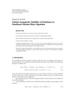
Figure 1: Magnitude spectrum showing: (a) an example of partially
colliding partials, and (b) an example of coincident partials.
as frequency and amplitude modulation. Using very short

time windows to perform the analysis over a period in
which the frequencies would be expected to be relatively
steady also does not work, as this procedure results in a very
coarse frequency resolution due to the well-known time-
frequency tradeoff. The problem is even more evident in the
case of coincident partials, because different partials vary in
different ways around a common frequency, making it nearly
impossible to accurately estimate their frequencies. However,
in most cases the band within which the partials are located
can be determined instead. Since the phase is usually ignored
and the frequency often cannot be reliably estimated due to
the time variations, it is the amplitude of individual partials
that can provide the most useful information to efficiently
separate coincident partials.
For the remainder of this paper, the term partial will
refer to a sinusoid with a frequency that varies with time. As
a result, the frequency band occupied by a partial during a
period of time will be given by the range of such a variation.
It is also important to note that the word partial can be
both used to indicate part of an individual source (isolated
harmonic), or part of the whole mixture—in this case, the
merging of two or more coincident partials would also be
called a partial. Partials referring to the mixture will be called
mixturepartials whenever the context does not resolve this
ambiguity.
The sinusoidal modeling technique can successfully esti-
mate the amplitudes when the partials of different sources do
not collide, but it loses its effectiveness when the frequencies
of the partials are close. The expression colliding partials
refers here to the cases in which two partials share at least part

of the spectrum (Figure 1(a)). The expression coincident
partials, on the other hand, is used when the colliding
partials are mostly concentrated in the same spectral band
(Figure 1(b)). In the first case, the partials may be separated
enough to generate some effects that can be explored to
resolve them, but in the second case they usually merge in
such a way they act as a single partial. In this work, two
partials will be considered coincident if their frequencies are
separated by less than 5% for frequencies below 500 Hz, and
by less than 25 Hz for frequencies above 500 Hz—according
to tests carried out previously, those values are roughly the
thresholds for which traditional techniques to resolve close
sinusoids start to fail. A small number of techniques to
resolve colliding partials have been proposed, and only a few
of them can deal with coincident partials.
Most techniques proposed in the literature can only
reliably resolve colliding partials if they are not coincident.
Klapuri et al. [26] explore the amplitude modulation result-
ing from two colliding partials to resolve their amplitudes.
If more than two partials collide, the standard interpolation
approach as described later is used instead. Virtanen and
Klapuri [27] propose a technique that iteratively estimates
phases, amplitudes, and frequencies of the partials using a
least-square solution. Parametric approaches like this one
tend to fail when the partials are very close, because some of
the matrices used to estimate the parameters tend to become
singular. The same kind of problem can occur in the strategy
proposed by Tolonen [16], which uses a nonlinear least-
squares estimation to determine the sinusoidal parameters
of the partials. Every and Szymanski [28] employ three

filter designs to separate partly overlapping partials. The
method does not work properly when the partials are mostly
concentrated in the same band. Hence, it cannot be used to
estimate the amplitudes of coincident or almost coincident
partials.
There are a few proposals that are able to resolve
coincident partials, but they only work properly under cer-
tain conditions. An efficient method to separate coincident
partials based on the similarity of the temporal envelopes was
proposed by Viste and Evangelista [29], but it only works
for multichannel mixtures. Duan et al. [30] use an average
harmonic structure (AHS) model to estimate the amplitudes
of coincident partials. To work properly, this method requires
that, at least for some frames, the partials be sufficiently
disjoint so their individual features can be extracted. Also,
the technique does not work when the frequencies of the
sources have octave relations. Woodruff et al. [31] propose a
technique based on the assumptions that harmonics of the
same source have correlated amplitude envelopes and that
phase differences can be predicted from the fundamental
frequencies. The main limitation of the technique is that it
depends on very accurate pitch estimates.
Since most of these elaborated methods usually have lim-
ited applicability, simpler and less constrained approaches
are often adopted instead. Some authors simply attribute all
the content to a single source [32], while others use a simple
interpolation approach [33–35]. The interpolation approach
estimates the amplitude of a given partial that is known to
be colliding with another one by linearly interpolating the
amplitudes of other partials belonging to the same source.

Several partials can be used in such an interpolation but,
according to Virtanen [25], normally only the two adjacent
ones are used, because they tend to be more correlated to
the amplitude of the overlapping partial. The advantage of
such a simple approach is that it can be used in almost
every case, with the only exceptions being those in which
the sources have the same fundamental frequency. On the
other hand, it has three main shortcomings: (a) it assumes
EURASIP Journal on Audio, Speech, and Music Processing 3
that both adjacent partials are not significantly changed
by the interference of other sources, which is often not
true; (b) the first partial (fundamental) cannot be estimated
using this procedure, because there is no previous partial
to be used in the interpolation; (c) the assumption that the
interpolation of the partials is a good estimate only holds for
a few instruments and, for the cases in which a number of
partials are practically nonexistent, such as a clarinet with
odd harmonics, the estimates can be completely wrong.
This paper presents a more refined alternative to the
interpolation approach, using some characteristics of the
harmonic audio signals to provide a better estimate for the
amplitudes of coincident partials. The proposal is based on
the hypothesis that the frequencies of the partials of a given
source will vary in approximately the same fashion over time.
In a short description, the algorithm tracks the frequency
of each mixture partial over time, and then uses the results
to calculate the correlations among the mixture partials.
The results are used to choose a reference partial for each
source, by determining which is the mixture partial that is
more likely to belong exclusively to that source, that is, the

partial with minimum interference from other sources. The
influence of each source over each mixture partial is then
determined by the correlation of the mixture partials with
respect to the reference partials. Finally, this information is
used to estimate how the amplitude of each mixture partial
should be split among its components.
This proposal has several advantages over the interpola-
tion approach.
(a) Instead of relying in the assumption that both
neighbor partials are interference-free, the algorithm
depends only on the existence of one partial strongly
dominated by each source to work properly, and
relatively reliable estimates are possible even if this
condition is not completely satisfied.
(b) The algorithm works even if the sources have the
same fundamental frequency (F0)—tests comparing
the spectral envelopes of a large number of pairs
of instruments playing the same note and having
the same RMS level, revealed that in 99.2% of the
cases there was at least one partial whose energy was
more than five times greater than the energy of its
counterpart.
(c) The first partial (fundamental) can be estimated.
(d) There are no intraframe permutation errors, mean-
ing that, assuming the amplitude estimates within a
frame are correct, they will always be assigned to the
correct source.
(e) The estimation accuracy is much greater than that
achieved by the interpolation approach.
In the context of this work, the term source refers

to a sound object with harmonic frequency structure.
Therefore, a vocal or an instrument generating a given note is
considered a source. This also means that the algorithm is not
able to deal with sound sources that do not have harmonic
characteristics, like percussion instruments.
The paper is organized as follows. Section 2 presents
the preprocessing. Section 3 describes all steps of the algo-
rithm. Section 4 presents the experiments and corresponding
results. Finally, Section 5 presents the conclusions and final
remarks.
2. Preprocessing
Figure 2 shows the basic structure of the algorithm. The
first three blocks, which represent the preprocessing, are
explained in this section. The last four blocks represent
the core of the algorithm and are described in Section 3.
The preprocessing steps described in the following are fairly
standard and have shown to be adequate for supporting the
algorithm.
2.1. Adaptive Frame Division. The first step of the algorithm
is dividing the signal into frames. This step is necessary
because the amplitude estimation is made in a frame-by-
frame basis. The best procedure here is to set the boundaries
of each frame at the points where an onset [36, 37](newnote,
instrument or vocal) occurs, so the longest homogeneous
frames are considered. The algorithm works better if the
onsets themselves are not included in the frame, because
during the period they occur, the frequencies may vary
wildly, interfering with the partial correlation procedure
described in Section 3.3. The algorithm presented in this
paper does not include an onset-detection procedure in order

to avoid cascaded errors, which would make it more difficult
to analyze the results. However, a study about the effects
of onset misplacements on the accuracy of the algorithm is
presented in Section 4.5.
To cope with partial amplitude variations that may occur
within a frame, the algorithm includes a procedure to divide
the original frame further, if necessary. The first condition
for a new division is that the duration of the note be at
least 200 ms, since dividing shorter frames would result in
frames too small to be properly analyzed. If this condition is
satisfied, the algorithm divides the original frame into two
frames, the first one having a 100-ms length, and the second
one comprising the remainder of the frame. The algorithm
then measures the RMS ratio between the frames according
to
R
RMS
=
min
(
r
1
, r
2
)
max
(
r
1
, r

2
)
,(1)
where r
1
and r
2
are the RMS of the first and second new
frames, respectively. R
RMS
will always assume a value between
zero and one. The RMS values were used here because
they are directly related to the actual amplitudes, which are
unknown at this point.
The R
RMS
value is then stored and a new division is
tested, now with the first new frame being 105-ms long and
the second being 5 ms shorter than it was originally. This
new R
RMS
value is stored and new divisions are tested by
successively increasing the length of the first frame by 5ms
and reducing the second one by 5 ms. This is done until the
4 EURASIP Journal on Audio, Speech, and Music Processing
Signal Estimates
Division into
frames
F0
estimation

Partial
filtering
Frame
subdivision
Segmental
frequency
estimation
Partial
correlation
Amplitude
estimation
procedure
Figure 2: Algorithm general structure.
resulting second frame is 100-ms long or shorter. If the lowest
R
RMS
value obtained is below 0.75 (empirically determined),
this indicates a considerable amplitude variation within
the frame, and the original frame is definitely divided
accordingly. If, as a result of this new division, one or both the
new frames have a length greater than 200 ms, the procedure
is repeated and new divisions may occur. This is done until
all frames are smaller than 200-ms, or until all possible R
RMS
values are above 0.75.
Some results using different fixed frame lengths are
presented in Section 4.
2.2. F0 Estimation and Partial Location. The position of the
partials of each source is directly linked to their fundamental
frequency (F0). The first versions of the algorithm included

the multiple fundamental frequencies estimator proposed by
Klapuri [38]. A common consequence of using supporting
tools in an algorithm is that the errors caused by flaws
inherent to those supporting tools will propagate throughout
the rest of the algorithm. Fundamental frequency errors are
indeed a problem in the more general context of sound
source separation, but since the scope of this paper is limited
to the amplitude estimation, errors coming from third-
party tools should not be taken into account in order to
avoid contamination of the results. On the other hand, if all
information provided by the supporting tools is assumed to
be known, all errors will be due to the proposed algorithm,
providing a more meaningful picture of its performance.
Accordingly, it is assumed that a hypothetical sound source
separation algorithm would eventually reach a point in
which the amplitude estimation would be necessary—to
reach this point, such an algorithm would maybe depend on
a reliable F0 estimator, but this is a problem that does not
concern this paper, so the correct fundamental frequencies
are assumed to be known.
Although F0 errors are not considered in the main tests,
it is instructive to discuss some of the impacts that F0
errors would have in the algorithm proposed here. Such a
discussion is presented in the following, and some practical
tests are presented in Section 4.6.
When the fundamental frequency of a source is mises-
timated, the direct consequence is that a number of false
partials (partials that do not exist in the actual signal, but
that are detected by the algorithm due to F0 estimation
error) will be considered and/or a number of real partials

will be ignored. F0 errors may have significant impact in the
estimation of the amplitudes of correct partials depending
on the characteristics of the error. Higher octave errors, in
which the detected F0 is actually a multiple of the correct one,
have very little impact on the estimation of correct partials.
This is because that, in this case, the algorithm will ignore
a number of partials, but those that are taken into account
are actual partials. Problems may arise when the algorithm
considers false partials, which can happen both in the case of
lower octave errors, in which the detected F0 is a submultiple
of the correct one, and in the case of nonoctave errors—this
last situation is the worst because most considered partials
are actually false, but fortunately this is the less frequent kind
of error. When the positions of those false partials coincide
with the positions of partials belonging to sources whose F0
were correctly identified, some problems may happen. As will
be seen in Section 3.4, the proposed amplitude estimation
procedure depends on the proper choice of reference partials
for each instrument, which are used as a template to estimate
the remaining ones. If the first reference partial to be chosen
belongs to the instrument for which the F0 was misestimated,
that has little impact on the amplitude estimation of the
real partials. On the other hand, if the first reference partial
belongs to the instrument with the correct F0, then the
entire amplitude estimation procedure may be disrupted.
The reasons for this behavior are presented in Section 4.6,
together with some results that illustrate how serious is the
impact of such a situation over the algorithm performance.
The discussion above is valid for significant F0 estimation
errors—precision errors, in which the estimated frequency

deviates by at most a few Hertz from the actual value, are
easily compensated by the algorithm as it uses a search width
of 0.1
· F0 around the estimated frequency to identify the
correct position of the partial.
As can be seen, considerable impact on the proposed
algorithm will occur mostly in the case of lower octave errors,
since they are relatively common and result in a number
of false partials—a study about this impact is presented in
Section 4.6.
To work properly, the algorithm needs a good estimate
of where each partial is located—the location or position of
a partial, in the context of this work, refers to the central
frequency of the band occupied by that partial (see definition
of partial in the introduction). Simply, taking multiples of F0
sometimes work, but the inherent inharmonicity [39, 40]of
some instruments may cause this approach to fail, especially
if one needs to take several partials into consideration. To
make the estimation of each partial frequency more accurate,
an algorithm was created—the algorithm is fed with the
frames of the signal and it outputs the position of the partials.
The steps of the algorithm for each F0 are the following:
(a) The expected (preliminary) position of each partial
(p
n
)isgivenbyp
n−1
+F0,withp
0
= 0.

(b) The short-time discrete Fourier transform (STDFT)
is calculated for each frame, from which the magni-
tude spectrum M is extracted.
EURASIP Journal on Audio, Speech, and Music Processing 5
(c) The adjusted position of the current partial (

p
n
)is
given by the highest peak in the interval [p
n
−s
w
, p
n
+
s
w
]ofM,wheres
w
= 0.1 · F0 is the search width.
This search width contains the correct position of the
partial in nearly 100% of the cases; a broader search
region was avoided in order to reduce the chance of
interference from other sources. If the position of the
partial is less than 2s
w
apart from any partial position
calculated previously for other source, and they are
not coincident (less than 5% or 25 Hz apart), the

positions of both partials are recalculated considering
s
w
equal to half the frequency distance among the two
partials.
When two partials are coincident in the mixed signal,
they often share the same peak, in which case steps (a) to
(c) will determine not their individual positions, but their
combined position, which is the position of the mixture
partial. Sometimes coincident partials may have discernible
separate peaks; however, they are so close that the algorithm
can take the highest one as the position of the mixture partial
without problem. After the positions of all partials related
to all fundamental frequencies have been estimated, they are
grouped into one single set containing the positions of all
mixture partials. The procedure described in this section has
led to partial frequency estimates that are within 5% from
the correct value (inferred manually) in more than 90% of
the cases, even when a very large number of partials are
considered.
2.3. Partial Filtering. The mixture partials for which the
amplitudes are to be estimated are isolated by means of a
filterbank. In real signals, a given partial usually occupies
a certain band of the spectrum, which can be broader or
narrower depending on a number of factors like instrument,
musician, and environment, among others. Therefore, a filter
with a narrow pass-band may be appropriate for some kinds
of sources, but may ignore relevant parts of the spectrum for
others. On the other hand, a broad pass-band will certainly
include the whole relevant portion of the spectrum, but may

also include spurious components resulting from noise and
even neighbor partials. Experiments have indicated that the
most appropriate band to be considered around the peak
of a partial is given by the interval [0.5
· (p
n−1
+ p
n
), 0.5 ·
(p
n
+ p
n+1
)], where p
n
is the frequency of the partial under
analysis, and p
n−1
and p
n+1
are the frequencies of the closest
partials with lower and higher frequencies, respectively.
The filterbank used to isolate the partials is composed by
third-order elliptic filters, with a passband ripple of 1 dB and
stopband attenuation of 80 dB. This kind of filter was chosen
because of its steep rolloff. Finite impulse response (FIR)
filters were also tested, but the results were practically the
same, with a considerably greater computational complexity.
As commented before, this method is intended to be
used in the context of sound source separation, whose

main objective is to resynthesize the sources as accurately as
possible. Estimating the amplitudes of coincident partials is
an important step toward such an objective, and ideally the
amplitudes of all partials should be estimated. In practice,
however, when partials have very low energy, noise plays
an important role, making it nearly impossible to extract
enough information to perform a meaningful estimate. As
a result of those observations, the algorithm only takes into
account partials whose energy—obtained by the integration
of the power spectrum within the respective band—is at
least 1% of the energy of the most energetic partial. Mixture
partials follow the same rules; that is, they will be considered
only if they have at least one percent of the energy the
strongest partial—thus, the energy of an individual partial
in a mixture may be below the 1% limit. It is important
to notice that partials below
−20 dB from the strongest one
may, in some cases, be relevant. Such a hard lower limit for
the partial energy is the best current solution for the problem
of noisy partials, but alternative strategies are currently under
investigation. In order to avoid that a partial be considered in
certain frames and not in others, if a given F0 keeps the same
in consecutive frames, the number of partials considered by
the algorithm is also kept the same.
3. The Proposed Algor ithm
3.1. Frame Subdivision. The resulting frames after the
filtering are subdivided into 10-ms subframes, with no
overlap (overlapping the sub-frames did not improve the
results). Longer sub-frames were not used because they may
not provide enough points for the subsequent correlation

calculation (see Section 3.3) to produce meaningful results.
On the other hand, if the sub-frame is too short and
the frequency is low, only a fraction of a period may
be considered in the frequency estimation described in
Section 3.2, making such estimation either unreliable, or
even impossible.
3.2. Partial Trajectory Estimation. The frequency of each
partial is expected to fluctuate over the analysis frame,
which have a length of at least 100 ms. Also, it is expected
that partials belonging to a given source will have similar
frequency trajectories, which can be explored to match
partials to that particular source. The 10-ms sub-frames
resulting from the division described in Section 3.1 are used
to estimate such a trajectory. The frequency estimation for
each 10-ms sub-frame is performed in the time domain by
taking the first and last zero-crossing, measuring the distance
d in seconds and the number of cycles c between those zero-
crossings, and then determining the frequency according to
f
= c/d. The exact position of the zero-crossing is given by
z
c
= p
1
+
|a
1
|·

p

2
− p
1

|a
1
| + |a
2
|
,
(2)
where p
1
and p
2
are, respectively, the positions in seconds
of the samples immediately before and immediately after the
zero-crossing, and a
1
and a
2
are the amplitudes of those same
samples. Once the frequencies for each 10-ms sub-frame are
calculated, they are accumulated into a partial trajectory.
6 EURASIP Journal on Audio, Speech, and Music Processing
−35
50 150 250 350 450 550 650 750 850
Frequency (Hz)
950
−30

−25
−20
Performance (in % of the mean accuracy)
−15
−10
−5
0
5
Figure 3: Effect of the frequency on the accuracy of the amplitude
estimates.
It is worth noting that there are more accurate tech-
niques to estimate a partial trajectory, like the normalized
cross-correlation [41]. However, replacing the zero-crossing
approach by the normalized cross-correlation resulted in
almost the same overall amplitude estimation accuracy
(mean error values differ by less than 1%), probably due
to artificial fluctuations in the frequency trajectory that are
introduced by the zero-crossing approach. Therefore, any of
the approaches can be used without significant impact on
the accuracy. The use of the zero-crossings, in this context,
is justified by the low computational complexity associated.
The use of sub-frames as small as 10-ms has some
important implications in the estimation of low frequencies.
Since at least two zero-crossings are necessary for the
estimates, the algorithm cannot deal with frequencies below
50 Hz. Also, below 150 Hz the partial trajectory shows some
fluctuations that may not be present in higher frequency
partials, thus reducing the correlation between partials and,
as a consequence, the accuracy of the algorithm. Figure 3
shows the effect of the frequency on the accuracy of the

amplitude estimates. In the plot, the vertical scale indicates
how better or worse is the performance for that frequency
with respect to the overall accuracy of the accuracy, in
percentage. As can be seen, for 100 Hz the accuracy of the
algorithm is 16% below average, and the accuracy drops
rapidly as lower frequencies are considered. However, as will
be seen in Section 4, the accuracy for such low frequencies is
still better than that achieved by the interpolation approach.
3.3. Partial Trajectory Correlation. The frequencies estimated
for each sub-frame are arranged into a vector, which
generates trajectories like those shown in Figure 4.One
trajectory is generated for each partial. The next step is
to calculate the correlation between each possible pair of
trajectories, resulting in N(N
−1)/2 correlation values, where
N is the number of partials.
3.4. Amplitude Estimation Procedure. The main hypothe-
sis motivating the procedure described here is that the
partial frequencies of a given instrument or vocal vary
approximately in the same way with time. Therefore, it is
hypothesized that the correlation between the trajectories of
two mixture partials will be high when they both belong
exclusively to a single source, with no interference from other
partials. Conversely, the lowest correlations are expected to
occur when the mixture partials are completely related to
different sources. Finally, when one partial results from a
given source A (called reference), and the other one results
from the merge of partials coming both from source A and
from other sources S, intermediary correlation values are
expected. More than that, it is assumed that the correlation

values will be proportional to the ratio a
A
/a
S
in the second
mixture partial, where a
A
is the amplitude of source A partial
and a
S
is the amplitude of the mixture partial with the source
A partial removed. If a
A
is much larger than a
S
, it is said that
the partial from source A dominates that band.
Lemma 1. Let A
1
= X
1
+N
1
and A
2
= X
2
+N
2
be independent

random variables, and let A
3
= aA
1
+ bA
2
be a random
variable representing their we ighted sum. Also, let X
1
, X
2
also
be independent random variables, and N
1
and N
2
be zero-mean
independe nt random variables. Finally, let
ρ
X,Y
=
cov
(
X, Y
)
σ
X
σ
Y
=

E

X − μ
X

Y − μ
Y

σ
X
σ
Y
(3)
be the cor relation coefficient between two random variables X
and Y with expected values μ
X
and μ
Y
and standard deviations
σ
X
and σ
Y
.Then,
ρ
A
1
,A
3
ρ

A
2
,A
3
=
a
b

σ
2
X
1
+ σ
2
N
1
σ
2
X
2
+ σ
2
N
2

⎛
⎝

σ
2

X
2
+ σ
2
N
2

σ
2
X
1
+ σ
2
N
1
⎞
⎠
. (4)
Assuming that σ
2
N
1
 σ
2
X
1
, σ
2
N
2

 σ
2
X
2
,andσ
X
1
≡ σ
X
2
, (4)
reduces to
ρ
A
1
,A
3
ρ
A
2
,A
3
=
a
b
.
(5)
For proof, see the appendix.
The lemma stated above can be directly applied to
the problem presented in this paper, as explained in the

following. First, a model is defined in which the nth partial
P
n
of an instrument is given by P
n
(t) = n · F0(t), where
F0(t) is the time-varying fundamental frequency and t is
the time index. In this idealized case, all partial frequency
trajectories would vary in perfect synchronism. In practice, it
is observed that the partial frequency trajectories indeed tend
to vary together, but factors like instrument characteristics,
room acoustics, and reverberation, among others, introduce
disturbances that prevent a perfect match between the
trajectories. Those disturbances can be modeled as noise,
so now P
n
(t) = n · F0(t)+N(t), where N is the noise.
If we consider both the fundamental frequency variations
F0(t) and the noisy disturbances N(t) as random variables,
the lemma applies—in this context, A
1
is the frequency
trajectory of a partial of instrument 1, given by the sum of
the ideal partial frequency trajectory X
1
and the disturbance
N
1
; A
2

is the frequency trajectory of a partial of instrument
2, which collides with the partial of instrument 1; A
3
is
the partial frequency trajectory resulting from the sum of
EURASIP Journal on Audio, Speech, and Music Processing 7
946
0 50 100 150 200 250 300 350
Second partial trajectory - instrument A
Time (ms)
400
947
948
Frequency (Hz)
949
950
951
952
953
(a)
1419
0 50 100 150 200 250 300 350
Third partial trajectory - instrument A
Time (ms)
400
1420
1421
1422
Frequency (Hz)
1423

1424
1425
1426
1427
1428
1429
(b)
955.5
0 50 100 150 200 250 300 350
Second partial trajectory - instrument B
Time (ms)
400
956
956.5
Frequency (Hz)
957
957.5
958
958.5
959
959.5
(c)
944
0 50 100 150 200 250 300 350
Second partial trajectory - mixture
Time (ms)
400
945
946
947

Frequency (Hz)
948
949
950
951
952
953
954
(d)
Figure 4: Trajectories (a) and (b) come from partials belonging to the same source, thus having very similar behaviors. Trajectory (c)
corresponds to a partial from another source. Trajectory (d) corresponds to a mixture partial; its characteristics result from the combination
of each partial trends, as well as from phase interactions between the partials. The correlation procedure aims to quantify how close the
mixture trajectory is from the behavior expected for each source.
the colliding partials. According to the lemma, the shape
of A
3
is the sum of the trajectories A
1
and A
2
weighted by
the corresponding amplitudes (a and b). In practice, this
assumption holds well when one of the partials has a much
larger amplitude than the other one. When the partials have
similar amplitudes, the resulting frequency trajectory may
differ from the weighted sum. This is not a serious problem
because such a difference is normally mild, and the algorithm
was designed to explore exactly the cases in which one partial
dominates the other ones.
It is important to emphasize that some possible flaws in

the model above were not overlooked: there are not many
samples to infer the model, the random variables are not IID
(independent and identically distributed), and the mixing
model is not perfect. However, the lemma and assumptions
stated before have as main objective to support the use of
cross-correlation to recover the mixing weights, for which
purpose they hold sufficiently well—this is confirmed by a
number of empirical experiments illustrated in Figures 4 and
5, which show how the correlation varies with respect to the
amplitude ratio between the reference source A and the other
sources. Figure 5 was generated using the database described
in the beginning of Section 4, in the following way:
(a) A partial from source A is taken as reference (h
r
).
(b) A second partial of source A is selected (h
a
), together
with a partial of same frequency from source B (h
b
).
(c) Mixture partials (h
m
) are generated according to w ·
h
a
+(1− w) · h
b
,wherew varies between zero and
one and represents the dominance of source A,as

represented in the horizontal axis of Figure 5. When
w is zero, source A is completely absent, and when
w is one, the partial from source A is completely
dominant.
(d) The correlation values between the frequency tra-
jectories of h
r
and h
m
are calculated and scaled in
such a way the normalized correlations are 0 and
1 when w
= 0andw = 1, respectively. The
scaling is performed according to (6), where C
ij
is the
correlation to be normalized, C
min
is the correlation
between the partial from source A and the mixture
when w
= 0, and C
max
is the correlation between the
partial from source A and the mixture when w
= 0—
in this case C
max
is always equal to one.
8 EURASIP Journal on Audio, Speech, and Music Processing

−1
00.10.20.30.40.50.60.70.8
Dominance of reference partial
0.9
−0.5
0
1
Normalised correlation
0.5
1
1.5
2
Figure 5: Relation between correlation of the frequency trajectories
and partial ratio.
If the hypothesis hold perfectly, the normalized corre-
lation would have always the same value of w (solid line
in Figure 5). As can be seen in Figure 5, the hypothesis
holds relatively well in most cases; however, there are some
instruments (particularly woodwinds) for which this tends
to fail. Further investigation will be necessary in order to
determine why this happens only for certain instruments.
The amplitude estimation procedure described next was
designed to mitigate the problems associated to the cases in
which the hypotheses tend to fail. As a result, the strategy
works fairly well if the hypotheses hold (partially or totally)
for at least one of the sources.
The amplitude estimation procedure can be divided into
two main parts: determination of reference partials and the
actual amplitude estimation, as described next.
3.4.1. Determination of Reference Partials. This part of the

algorithm aims to find the partials that best represent each
source in the mixture. The objective is to find the partials
that are less affected by sources other than the one it should
represent. The use of reference partials for each source
guarantees that the estimated amplitudes within a frame will
be correctly grouped. As a result, no intraframe permutation
errors can occur. It is important to highlight that this paper
is devoted to be problem of estimating the amplitudes for
individual frames. A subsequent problem would be taking
all frame-wise amplitude estimates within the whole signal
and assign them to the correct sources. A solution for this
problem based on musical theory and continuity rules is
expected to be investigated in the future.
In order to illustrate how the reference partials are
determined, consider a hypothetical signal generated by
two simultaneous instruments playing the same note. Also,
consider that all mixture partials after the fifth have negligible
amplitudes. Ta bl e 1 shows the frequency correlation values
between the partials of this hypothetical signal, as well as
the amplitude of each mixture partial. The values between
parentheses are the warped correlation values, calculated
according to
C

ij
=
C
ij
− C
min

C
max
− C
min
,
(6)
where C
ij
is the correlation value (between partials i and
j) to be warped, and C
min
and C
max
are the minimum and
maximum correlation values for that frame. As a result, all
correlation values now lie between 0 and 1, and the relative
differences among the correlation values are reinforced.
ThevaluesinTab le 1 are used as example to illustrate
each step of the procedure to determine the amplitude of
each source and partial. Although the example considers
mixtures of only two instruments, the rules are valid for any
number of simultaneous instruments.
(a) If a given source has some partials that do not
coincide with any other partial, which is determined
using the results of the partial positioning procedure
described in Section 2.2, the most energetic among
such partials is taken as reference for that source. If
all sources have at least one of such “clean” partials
to be taken as reference, the algorithm skips directly
to the amplitude estimation. If at least one source

satisfies the “clean partial” condition, the algorithm
skips to item (d), and the most energetic reference
partial is taken as the global reference partial G.Items
(b) and (c) only take place if no source satisfies such a
condition, which is the case of the hypothetical signal.
(b) The two mixture partials that result in the greatest
correlation are selected (first and third in Ta bl e 1).
Those are the mixture partials for which the fre-
quency variations are more alike, which indicates that
they both belong mostly to a same source. In this case,
possible coincident partials have small amplitudes
compared to the dominant partials.
(c) The most energetic among those two partials is
chosen both as the global reference G and as reference
for the corresponding source, as the partial with
greatest amplitude probably has the most defined
features to be compared to the remaining ones. In the
example given by Tabl e 1, the first partial is taken as
reference R
1
for instrument 1 (R
1
= 1).
(d) In this step, the algorithm chooses the reference
partials for the remaining sources. Let I
G
be the
source of partial G, and let I
C
be the current source

for which the reference partial is to be determined.
The reference partial for I
C
is chosen by taking the
mixture partial that result in the lowest correlation
with respect to G, provided that the components of
such mixture partial belong only to I
C
and I
G
(if no
partial satisfies this condition, item (e) takes place).
As a result, the algorithm selects the mixture partial
in which I
C
is more dominant with respect to I
G
.In
the example shown in Tab le 1 , the fourth partial has
the lowest correlation with respect to G(
−0.3), being
taken as reference R
2
for instrument 2 (R
2
= 4).
EURASIP Journal on Audio, Speech, and Music Processing 9
Table 1: Illustration of the amplitude estimation procedure. If the last row is removed, the table is a matrix showing the correlations between
the mixture partials, and the values between parentheses are the warped correlation values according to (6). Thus, the regular and warped
correlations between partials 1 and 2 are, respectively, 0.2 and 0.62. As can be seen, the lowest correlation value overall will have a warped

correlation of 0, and the highest correlation value is warped to 1; all other correlations will have intermediate warped value. The last row in
the table reveals the amplitude of each one of the mixture partials.
Partial12345
1—0.2(0.62) 0.5 (1.0) −0.3(0.0) 0 (0.37)
2 — — 0.1 (0.5)
−0.1(0.25) −0.2(0.12)
3———
−0.2(0.12) −0.2(0.12)
4 — — — — 0.1 (0.5)
5 —————
Amp. 0.7 0.9 0.4 0.5 0.3
(e) This item takes place if all mixture partials are
composed by at least three instruments. In this
case, the mixture partial that result in the lowest
correlation with respect to G is chosen to represent
the partial least affected by I
G
.Theobjectivenowis
to remove from the process all partials significantly
influenced by I
G
.Thisiscarriedoutbyremoving
all partials whose warped correlation values with
respect to R
1
are greater than half the largest warped
correlation value of R
1
. In the example given by
Ta ble 1 , the largest warped correlation would be 1,

and partials 2 and 3 would be removed accordingly.
Then, items (a) to (d) are repeated for the remaining
partials. If more than two instruments still remain
in the process, item (e) takes place once more, and
the process continues until all reference partials have
been determined.
3.4.2. Amplitude Estimation. The reference partials for each
source are now used to estimate the relative amplitude to be
assigned to each partial of each source, according to
A
s
(
i
)
=
C

i,R
s

N
n=1
C

i,R
n
,
(7)
where A
s

indicate the relative amplitude to be assigned to
source s in the mixture partial, n is the index of the source
(considering only the sources that are part of that mixture),
and C

ij
is the warped correlation value between partials i
and j. The warped correlation were used because, as pointed
out before, they enhance the relative differences among the
correlations. As can be seen in (7), the relative amplitudes
to be assigned to the partials in the mixture are directly
proportional to the warped correlations of the partial with
respect to the reference partials. This reflects the hypothesis
that higher correlation values indicate a stronger relative
presence of a given instrument in the mixture. Ta ble 2 shows
the relative partial amplitudes for the example given by
Ta ble 1 .
As can be seen, both (6)and(7) are heuristic. They were
determined empirically by a thorough observation of the
data and exhaustive tests. Other strategies, both heuristic and
statistical, were tested, but this simple approach resulted in a
performance comparable to those achieved by more complex
strategies.
In the following, the relative partial amplitudes are used
to extract the amplitudes of each individual partial from the
mixture partial (values between parentheses). In the exam-
ple, the amplitude of the mixture partial is assumed to be
equal to the sum of the amplitudes of the coincident partials.
This would only hold if the phases of coincident partials were
aligned, which in practice does not occur. Ideally, amplitude

and phase should be estimated together to produce accurate
estimates. However, the characteristics of the algorithm made
it necessary the adoption of simplifications and assumptions
that, if uncompensated, might result in inaccurate estimates.
To compensate (at least partially) the phase being neglected
in previous steps of the algorithm, some further processing is
necessary: a rough estimate of which amplitude the mixture
would have if the phases were actually perfectly aligned is
obtained by summing the amplitudes estimated using part of
the algorithm proposed by Yeh and Roebel [42] in Sections
2.1and2.2 of their paper. This rough estimate is, in general,
larger than the actual amplitude of the mixture partial. This
difference between both amplitudes is a rough measure of the
phase displacement between the partials. To compensate for
such a phase displacement, a weighting factor given by w
=
A
r
/A
m
,whereA
r
is the rough amplitude estimate and A
m
is
the actual amplitude of the mixture partial and is multiplied
to the initial zero-phase partial amplitude estimates. This
procedure improves the accuracy of the estimates by about
10%.
As a final remark, it is important to emphasize that

the amplitudes within a frame are not constant. In fact,
the proposed method explores the frequency modulation
(FM) of the signals, and FM is often associated with
some kind of amplitude modulation (AM). However, the
intraframe amplitude variations are usually small (except
in some cases of strong vibrato), making it reasonable
to estimate an average amplitude instead of detecting the
exact amplitude envelope, which would be a task close to
impossible.
10 EURASIP Journal on Audio, Speech, and Music Processing
Table 2: Relative and corresponding effective partial amplitudes (between parentheses). The relative amplitudes reveal which percentage
of the mixture partial should be assigned to each source, hence the sum in each column is always 1 (100%). The effective amplitudes are
obtained by multiplying the relative amplitudes by the mixture partial amplitudes shown in the last row of Tab le 1 ,hencethesumofeach
column in this case is equal to the amplitudes shown in the last row of Tabl e 1 .
Partial 1 2 3 4 5
Inst. 1 1 (0.7) 0.71 (0.64) 0.89 (0.36) 0 (0) 0.43 (0.13)
Inst. 2 0 (0) 0.29 (0.26) 0.11 (0.04) 1 (0.5) 0.57 (0.17)
4. Experimental Results
The mixtures used in the tests were generated by summing
individual notes taken from the instrument samples present
in the RWC database [43]. Eighteen instruments of several
types (winds, bowed strings, plucked strings, and struck
strings) were considered—mixtures including both vocals
and instruments were tested separately, as described in
Section 4.7. In total, 40156 mixtures of two instruments,
three, four and five instruments were used in the tests.
The mixtures of two sources are composed by instruments
playing in unison (same note), and the other mixtures
include different octave relations (including unison). A
mixture can be composed by the same kind of instrument.

Those settings were chosen in order to test the algorithm
with the hardest possible conditions. All signals are sampled
at 44.1 kHz, and have a minimum duration of 800 ms. Next
subsections present the main results according to different
performance aspects.
4.1. Overall Performance and Comparison with Interpolation
Approach. Tabl e 3 shows the mean RMS amplitude error
resulting from the amplitude estimation of the first 12
partials in mixtures with two to five instruments (I2 to I5 in
the first column). The error is given in dB and is calculated
according to
error
=
E
abs
A
max
,
(8)
where E
abs
is the absolute error between the estimate and
the correct amplitude, and A
max
is the amplitude of the
most energetic partial. The error values for the interpolation
approach were obtained by taking an individual instrument
playing a single note, and then measuring the error between
the estimate resulting from the interpolation of the neighbor
partials and the actual value of the partial. This represents

the ideal condition for the interpolation approach, since the
partials are not disturbed at all by other sources. The inherent
dependency of the interpolation approach on clean partials
makes its use very limited in real situations, especially if
several instruments are present. This must be taken into
consideration when comparing the results in Ta ble 3 .
In Tab le 3, the partial amplitudes of each signal were
normalized so the most energetic partial has a RMS value
equal to 1. No noise besides that naturally occurring in the
recordings was added, and the RMS values of the sources
have a 1 : 1 ratio.
The results for higher partials are not shown in Tabl e 3
in order to improve the legibility of the results. Additionally,
their amplitudes are usually small, and so is their absolute
error, thus including their results would not add much
information. Finally, due to the rules defined in Section 2.2,
normally only a few partials above the twelfth are considered.
As a consequence, higher partials will have much less results
to be averaged, thus their results are less significant. Only
one line was dedicated to the interpolation approach because
the ideal conditions adopted in the tests make the number of
instruments in the mixture irrelevant.
The total errors presented in Ta bl e 3 were calculated
taking only the 12 first partials into consideration. The
remaining partials were not considered because their only
effect would be reducing the total error value.
Before comparing the techniques, there are some impor-
tant remarks to be made about the results shown in Tab le 3 .
As can be seen, for both techniques the mean errors are
smaller for higher partials. This is not because they are

more effective in those cases, but because the amplitudes
of higher partials tend to be smaller, and so does the error,
since it is calculated having the most energetic partial as
reference. As a response, new error rates—called modified
mean error—were calculated for two-instrument mixtures
using as reference the average amplitude of the partials, as
shown in Ta bl e 4—the error values for the other mixtures
were omitted because they have approximately the same
behavior. The modified errors are calculated as in (8), but
in this case A
max
is replaced by the average amplitude of the
12 partials.
As stated before, the results for the interpolation
approach were obtained under ideal conditions. Also, it
is important to note that the first partial is often the
most energetic one, resulting in greater absolute errors.
Since the interpolation procedure cannot estimate the first
partial, it is not part of the total error. In real situations
with different kinds of mixtures present, the results for the
interpolation approach could be significantly worse. As can
be seen in Tab le 3, although facing harder conditions, the
proposed strategy outperforms the interpolation approach
even when dealing with several simultaneous instruments.
This indicates that the relative improvement achieved by the
proposed algorithm with respect to the interpolation method
is significant.
As expected, the best results were achieved for mixtures
of two instruments. The accuracy degrades when more
instruments are considered, but meaningful estimates can be

obtained for up to five simultaneous instruments. Although
the algorithm can, in theory, deal with mixtures of six
or more instruments, in such cases the spectrum tends to
become too crowded for the algorithm to work properly.
EURASIP Journal on Audio, Speech, and Music Processing 11
Table 3: Mean error comparison between the proposed algorithm and the interpolation approach (in dB).
Partial123456789101112Total
I2 −7.1 −8.5 −9.7 −11.2 −12.3 −13.7 −14.8 −15.9 −17.0 −17.5 −18.3 −19.2 −12.0
I3
−5.4 −6.7 −7.9 −9.4 −10.3 −11.9 −12.8 −13.9 −14.8 −15.6 −16.2 −17.0 −10.2
I4
−4.8 −6.1 −7.4 −8.8 −9.9 −11.2 −12.4 −13.4 −14.1 −15.0 −15.6 −16.0 −9.6
I5
−4.5 −5.8 −7.0 −8.4 −9.5 −10.8 −12.0 −12.9 −13.6 −14.5 −14.8 −15.2 −9.2
Interp.
a
−4.6 −6.2 −7.7 −8.9 −9.9 −10.3 −10.6 −11.0 −10.8 −10.5 −10.5 −8.6
a
First partial cannot be estimated.
Table 4: Modified mean error values in dB.
Partial123456789101112Total
Prop. −5.4 −5.3 −5.8 −5.9 −6.0 −6.1 −6.4 −6.3 −6.6 −6.4 −6.6 −6.8 −6.1
Analyzing specifically Ta bl e 4, it can be observed that the
performance of the proposed method is slightly better for
higher partials.
This is because the mixtures in Tab le 4 were generated
using instruments playing the same notes, and higher partials
in that kind of mixture are more likely to be strongly
dominated by one of the instruments—most instruments
have strong low partials, so they will all have significant

contributions in the lower partials of the mixture. Mixture
partials that are strongly dominated by a single instrument
normally result in better amplitude estimates, because they
correlate well with the reference partials, explaining the
results shown in Ta bl e 4.
From this point to the end of Section 4, all results were
obtained using two-instrument mixtures—other mixtures
were not included to avoid redundancy.
4.2. Performance Under Noisy Conditions. Ta bl e 5 shows the
performance of the proposal when the signals are corrupted
by additive white noise. The results were obtained by
artificially summing the white noise to the mixtures of two
signals used in Section 4.1.
As can be seen, the performance is only weakly affected
by noise. The error rates only begin to rise significantly
close to 0 dB but, even under such an extremely noisy
condition, the error rate is only 25% greater than that
achieved without any noise. Such a remarkable robustness to
noise probably happens because, although noise introduces
a random factor in the frequency tracking described in
Section 3.2, the frequency variation tendencies are still able
to stand out.
4.3. Influence of RMS Ratio. Ta bl e 6 shows the performance
of the proposal for different RMS ratios between the sources.
The signals were generated as described in Section 4.1,but
scaling one of the sources to result in the RMS ratios shown
in Ta bl e 6. As can be seen, the RMS ratio between the sources
has little impact on the performance of the strategy.
4.4. Length of the Frames. As stated in Section 2.1, the best
way to get the most reliable results is to divide the signal in

frames with variable lengths according to the occurrence of
onsets. Therefore, it is useful to determine how dependent
the performance is to the frame length. Tabl e 7 shows the
results for different fixed frame lengths. The signals were
generated by simply taking the two-partial mixtures used in
Section 4.1 and truncating the frames to the lengths shown
in Ta ble 7 .
As expected, the performance degrades as shorter frames
are considered because there is less information available,
making the estimates less reliable. The interpolation results
are affected in almost the same way, which indicates that
this is indeed a matter of lack of information, and not
a problem related to the characteristics of the algorithm.
Future algorithm improvements may include a way of
exploring the information contained in other frames to
counteract the damaging effects of using short frames.
4.5. Onset Errors. This section analyses the effects of onset
misplacements. The following kinds of onset location errors
may occur.
(a) Small errors: errors smaller than 10% of the frame
length have little impact in the accuracy of the
amplitude estimates. If the onset is placed after the
actual position, a small section of the actual frame
will be discarded, in which case there is virtually no
loss. If the onset is placed before the actual position,
a small section of other note may be considered,
slightly affecting the correlation values. This kind of
mistake increases the amplitude estimation error in
about 2%.
(b) Large errors, estimated onset placed after the actual

position: the main consequence of this kind of
mistake is that fewer points are available in the
calculation of the correlations, which has a relatively
mild impact in the accuracy. For instruments whose
notes decay with time, like piano and guitar, a more
damaging consequence is that the most relevant part
of the signal may not be considered in the frame.
The main problem here is that after the note decays
by a certain amount, the frequency fluctuations in
different partials may begin to decorrelate. Therefore,
12 EURASIP Journal on Audio, Speech, and Music Processing
Table 5: Mean error values in dB for different noise levels.
SNR (dB) 60+ 50 40 30 20 10 0
Error (dB) −12.0 −12.0 −12.0 −12.0 −11.9 −11.8 −11.0
Table 6: Mean error in dB for different RMS ratios.
Ratio 1:1 1:0.9 1:0.7 1:0.5 1:0.3
Error (dB) −12.0 −12.0 −12.0 −12.2 −11.8
Table 7: Mean error in dB for different frame lengths.
Length (s) 1 0.5 0.2 0.1
Proposal −12.0 −11.7 −11.3 −10.8
Interpol.
−8.6 −8.4 −8.0 −7.6
if the strongest part of the note is not considered,
the results tend to be worse. Figure 6 shows the
dependency of the RMSE values on the extent of the
onset misplacements. The results shown in the figure
were obtained exactly in the same way as those in
Section 4.1, but deliberately misplacing the onsets to
reveal the effects of this kind of error.
(c) Large errors, estimated onset placed before the actual

position: in this case, a part of the signal that does
not contain the new note is considered. The effect of
this kind of error is that many points that should not
be considered in the correlation calculation are taken
into account. As can be seen in Figure 6, the larger is
the error, the worse is the amplitude estimate.
There are other kinds of onset errors besides
positioning—missing and spurious onsets. The analysis
of those kinds of errors is analog to that presented to the
onset location errors. The effect of spurious onset is that
the note will be divided into additional segments, so there
will be fewer points available for the calculation, and the
observations presented in item (b) hold. In the case of
missing onset, two segments containing different notes will
be considered, in a situation that is similar to that discussed
in item (c).
4.6. Impact of Lower Octave Errors. As stated in Section 2.2,
lower octave errors may affect the accuracy of the proposed
algorithm when this is cascaded with a F0 estimator. Ta bl e 8
shows the algorithm accuracy for the actual partials when the
estimated F0 for one of them is one, two or three octaves
below the actual value. As commented before, the lower
octave errors usually introduce a number of low correlations
that are mistakenly taken into account in the amplitude
estimation procedure described in Section 3.4. Since the
choice of the first reference partial is based on the highest
correlation, it is not usually affected by the lower octave
error. If this first reference partial belongs to the instrument
for which the fundamental frequency was misestimated, the
choice of the other reference partial will also not be affected,

because in this case all potential partials actually belong to
the instrument. Also, all correlations considered in this case
01020
Error after actual onset position-sustained instruments
Error after actual onset position-decaying instruments
Error before actual onset position
30 40 50 60
Position error in percentage of the actual ideal frame
70
−11
−12
−10
80
Mean error (dB)
−9
−8
−7
−6
Figure 6: Impact of onset misplacements in the accuracy of the
proposed algorithm.
are valid, as they are related to the first reference partial. As a
result, the accuracy of amplitude estimates is not affected.
Problems occur when the first reference partial belongs
to the instrument whose F0 was correctly estimated. In this
case, several false potential partials will be considered in the
process to determine the second reference partial, which is
chosen based on the lowest correlation. Since those false
partials are expected to have very low correlations with
respect to all other partials, the chance of one of them
being taken as reference is high. In this case, all the process

is disrupted and the amplitude estimates are likely to be
wrong. This explains the deterioration of the results shown in
Ta ble 8 . Those observations can be extended to mixtures with
any number of instruments, and the higher is the number of
F0 misestimates, the worse will be the results.
4.7. Separating Vocals. The mixtures used in this section were
generated by taking vocal samples from the RWC instrument
database [43] and adding an accompanying instrument or
another vocal. Therefore, all mixtures are composed by two
sources, with at least one being a vocal sample. Several notes
of all 18 instruments were considered, and they were all
scaled to have the same RMS value as the vocal sample.
Ta ble 9 shows the results when the algorithm was applied to
separate vocals from the accompanying instruments (second
row) and from other vocals (third row). The vocals were
produced by male and female adults with different pitch
ranges (soprano, alto, tenor, baritone and bass), and consist
of vowels being verbalized in a sustained way.
The results shown in Ta bl e 9 refer only to the vocal
sources, and the conditions are the same as those used to
generate Ta bl e 3.
EURASIP Journal on Audio, Speech, and Music Processing 13
Table 8: Mean error in dB for some lower octave errors.
Partial123456789101112Total
no error −7.1 −8.5 −9.7 −11.2 −12.2 −13.6 −14.8 −15.9 −17.1 −17.3 −18.2 −18.2 −12.0
1octave
−5.9 −7.3 −8.5 −10.1 −11.1 −12.5 −13.6 −14.7 −15.9 −15.9 −17.1 −17.3 −10.8
2octaves
−5.3 −6.7 −7.9 −9.5 −10.4 −11.9 −13.1 −14.1 −15.5 −15.4 −16.4 −16.3 −10.4
3octaves

−4.8 −6.2 −7.3 −9.1 −9.9 −11.4 −12.5 −13.6 −14.9 −14.9 −15.7 −15.9 −9.8
Table 9: Mean error in dB for vocal signals.
Partial123456789101112Total
V × I −7.2 −8.2 −9.9 −11.2 −12.5 −13.5 −13.9 −14.3 −14.3 −14.2 −14.2 −14.3 −11.5
V
× V −6.9 −7.9 −9.6 −10.8 −11.9 −13.0 −13.2 −13.8 −13.6 −13.5 −13.5 −13.6 −11.1
As can be seen, the results for vocal sources are only
slightly worse than those achieved for musical instruments.
This indicates that the algorithm is also suitable for dealing
with vocal signals. Future work will try to extend the
technique to the speech separation problem.
4.8. Final Remarks. The problem of estimating the amplitude
of coincident partials is a very difficult one. More than
that, this is a technology in its infancy. In that context,
many of the solutions adopted did not perform perfectly,
and there are some pathological cases in which the method
tends to fail completely. However, the algorithm performs
reasonably well in most cases, which shows its potentiality.
Since this is a technology far from mature, each part
of the algorithm will probably be under scrutiny in the
near future. The main motivation for this paper was to
propose a completely different way of tackling the problem of
amplitude estimation, highlighting its strong characteristics
and pointing out the aspects that still need improvement.
In short, this paper was intended to be a starting point
in the development of a new family of algorithms capable
of overcoming some the main difficulties currently faced
by both amplitude estimation and sound source separation
algorithms.
5. Conclusions

This paper presented a new strategy to estimate the
amplitudes of coincident partials. The proposal has several
advantages over its predecessors, such as better accuracy, the
ability to estimate the first partial, reliable estimates even
if the instruments are playing the same note, and so forth.
Additionally, the strategy is robust to noise and is able to deal
with any number of simultaneous instruments.
Although it presents a better performance than its
predecessor, there is still room for improvement. Future
versions may include new procedures to refine the estimates,
like using the information from previous frames to verify
the consistency of the current estimates. The extension of
the technique to the speech separation problem is currently
under investigation.
Appendix
Proof of Lemma 1
Let A
1
= X
1
+ N
1
and A
2
= X
2
+ N
2
,whereX
1

and X
2
are
random variables representing the actual partial frequency
trajectory, and N
1
and N
2
are random variables representing
the zero-mean, independent noise associated. Then, A
3
=
aA
1
+ bA
2
= aX
1
+ bX
2
+ aN
1
+ bN
2
and
ρ
A
1
,A
3

ρ
A
2
,A
3
=
E
(
A
1
A
3
)
− E
(
A
1
)
E
(
A
3
)
σ
A
1
σ
A
3
·

σ
A
2
σ
A
3
E
(
A
2
A
3
)
− E
(
A
2
)
E
(
A
3
)
,
(A.1)
In the following, each term of (A.1)isexpanded:
E
(
A
1

· A
3
)
= E
[
(
X
1
+ N
1
)
·
(
aX
1
+ bX
2
+ aN
1
+ bN
2
)
]
= aE

X
2
1

+ bE

(
X
1
)
E
(
X
2
)
+ aE

N
2
1

.
(A.2)
The terms aE
2
(X
1
)andaE
2
(N
1
) are then summed and
subtracted to the expression, keeping it unaltered. This is
done to explore the relation σ
2
X

= E(X
2
) − E
2
(X) and,
assuming that E(N
1
) = 0andE(N
2
) = 0, the expression
becomes
E
(
A
1
· A
3
)
= aE

X
2
1

+ bE
(
X
1
)
E

(
X
2
)
+ aE

N
2
1

+ aE
2
(X
1
) − aE
2
(X
1
)
  
=0
+ aE
2
(N
1
) − aE
2
(N
1
)

  
=0
= aE

X
2
1

− aE
2
(
X
1
)
+ bE
(
X
1
)
E
(
X
2
)
+ aE

N
2
1


−
aE
2
(
N
1
)
+ aE
2
(N
1
)
  
=0
+ aE
2
(
X
1
)
= aσ
2
X
1
+ bE
(
X
1
)
E

(
X
2
)
+ aσ
2
N
1
+ aE
2
(
X
1
)
.
(A.3)
Following the same steps,
E
(
A
2
· A
3
)
= bσ
2
X
2
+ aE
(

X
1
)
E
(
X
2
)
+ bσ
2
N
2
+ bE
2
(
X
2
)
. (A.4)
14 EURASIP Journal on Audio, Speech, and Music Processing
The other terms are given by
E
(
A
1
)
· E
(
A
3

)
= E
(
X
1
)(
aE
(
X
1
)
+ bE
(
X
2
))
= aE
2
(
X
1
)
+ bE
(
X
1
)
E
(
X

2
)
,
E
(
A
2
)
· E
(
A
3
)
= E
(
X
2
)(
aE
(
X
1
)
+ bE
(
X
2
))
= bE
2

(
X
2
)
+ aE
(
X
1
)
E
(
X
2
)
.
(A.5)
Substituting all these terms in (A.1) and eliminating self-
cancelling terms, the expression becomes
ρ
A
1
,A
3
ρ
A
2
,A
3
=
a ·


σ
2
X
1
+ σ
2
N
1

b ·

σ
2
X
2
+ σ
2
N
2

·
σ
A
2
σ
A
1
. (A.6)
Considering that σ

2
A
1
= σ
2
X
1
+ σ
2
N
1
and σ
2
A
2
= σ
2
X
2
+ σ
2
N
2
,
then
ρ
A
1
,A
3

ρ
A
2
,A
3
=
a ·

σ
2
X
1
+ σ
2
N
1

b ·

σ
2
X
2
+ σ
2
N
2

·


σ
2
X
2
+ σ
2
N
2

σ
2
X
1
+ σ
2
N
1
. (A.7)
If σ
2
N
1
 σ
2
X
1
and σ
2
N
2

 σ
2
X
2
, then
ρ
A
1
,A
3
ρ
A
2
,A
3
=
a
b
·
σ
2
X
1
σ
2
X
2
·
σ
X

2
σ
X
1
=
a
b
·
σ
X
1
σ
X
2
. (A.8)
Aditionally if σ
X
1
≡ σ
X
2
,
ρ
A
1
,A
3
ρ
A
2

,A
3
=
a
b
.
(A.9)
Acknowledgments
Special thanks are extended to Foreign Affairs and Inter-
national Trade Canada for supporting this work under its
Post-Doctoral Research Fellowship Program (PDRF). The
authors also would like to thank Dr. Sudhakar Ganti for his
help. Work was performed while the first author was with
the Department of Computer Science, University of Victoria,
Canada.
References
[1] K. Kokkinakis and A. K. Nandi, “Multichannel blind decon-
volution for source separation in convolutive mixtures of
speech,” IEEE Transactions on Audio, Speech and Language
Processing, vol. 14, no. 1, pp. 200–212, 2006.
[2] H. Saruwatari, T. Kawamura, T. Nishikawa, A. Lee, and K.
Shikano, “Blind source separation based on a fast-convergence
algorithm combining ICA and beamforming,” IEEE Transac-
tions on Audio, Speech and Language Processing, vol. 14, no. 2,
pp. 666–678, 2006.
[3]T.Kim,H.T.Attias,S Y.Lee,andT W.Lee,“Blindsource
separation exploiting higher-order frequency dependencies,”
IEEE Transactions on Audio, Speech and Language Processing,
vol. 15, no. 1, pp. 70–79, 2007.
[4] S.C.Douglas,M.Gupta,H.Sawada,andS.Makino,“Spatio-

temporal FastICA algorithms for the blind separation of
convolutive mixtures,” IEEE Transactions on Audio, Speech and
Language Processing, vol. 15, no. 5, pp. 1511–1520, 2007.
[5] N. Roman and D. Wang, “Pitch-based monaural segregation
of reverberant speech,” Journal of the Acoustical Society of
America, vol. 120, no. 1, pp. 458–469, 2006.
[6]
¨
O. Yilmaz and S. Rickard, “Blind separation of speech
mixtures via time-frequency masking,” IEEE Transactions on
Signal Processing, vol. 52, no. 7, pp. 1830–1846, 2004.
[7] M. H. Radfar and R. M. Dansereau, “Single-channel speech
separation using soft mask filtering,” IEEE Transactions on
Audio, Speech and Language Processing, vol. 15, no. 8, pp. 2299–
2310, 2007.
[8] R. Saab,
¨
O. Yilmaz, M. J. McKeown, and R. Abugharbieh,
“Underdetermined anechoic blind source separation via 
q
-
basis-pursuit With q
 1,” IEEE Transactions on Signal
Processing, vol. 55, no. 8, pp. 4004–4017, 2007.
[9] A. A
¨
ıssa-El-Bey, N. Linh-Trung, K. Abed-Meraim, A.
Belouchrani, and Y. Grenier, “Underdetermined blind sepa-
ration of nondisjoint sources in the time-frequency domain,”
IEEE Transactions on Signal Processing, vol. 55, no. 3, pp. 897–

907, 2007.
[10] A. A
¨
ıssa-El-Bey, K. Abed-Meraim, and Y. Grenier, “Blind
separation of underdetermined convolutive mixtures using
their time-frequency representation,” IEEE Transactions on
Audio, Speech and Language Processing, vol. 15, no. 5, pp. 1540–
1550, 2007.
[11] M. K. I. Molla and K. Hirose, “Single-mixture audio source
separation by subspace decomposition of hilbert spectrum,”
IEEE Transactions on Audio, Speech and Language Processing,
vol. 15, no. 3, pp. 893–900, 2007.
[12] A. Abramson and I. Cohen, “Single-sensor audio source
separation using classification and estimation approach and
GARCH modeling,” IEEE Transactions on Audio, Speech and
Language Processing, vol. 16, no. 8, pp. 1528–1540, 2008.
[13] Y. Li and D. Wang, “Separation of singing voice from music
accompaniment for monaural recordings,” IEEE Transactions
on Audio, Speech and Language Processing,vol.15,no.4,pp.
1475–1487, 2007.
[14] T. Virtanen, “Monaural sound source separation by non-
negative matrix factorization with temporal continuity and
sparseness criteria,” IEEE Transactions on Audio, Speech and
Language Processing, vol. 15, no. 3, pp. 1066–1074, 2007.
[15] L. Benaroya, F. Bimbot, and R. Gribonval, “Audio source
separation with a single sensor,” IEEE Transactions on Audio,
Speech and Language Processing, vol. 14, no. 1, pp. 191–199,
2006.
[16] T. Tolonen, “Methods for separation of harmonic sound
sources using sinusoidal modeling,” in Proceedings of the Audio

Engineering Society Convention, May 1999, preprint 4958.
[17] K. Itoyama, M. Goto, K. Komatani, T. Ogata, and H. G.
Okuno, “Integration and adaptation of harmonic and inhar-
monic models for separating polyphonic musical signals,”
in Proceedings of IEEE International Conference on Acoustics,
Speech and Signal Processing (ICASSP ’07), pp. 57–60, April
2007.
[18] L. Benaroya, L. M. Donagh, F. Bimbot, and R. Gribonval, “Non
negative sparse representation for Wiener based source separa-
tion with a single sensor,” in Proceedings of IEEE International
Conference on Acoustics, Speech, and Signal Processing (ICASSP
’03), pp. 613–616, April 2003.
[19] J. J. Burred and T. Sikora, “On the use of auditory rep-
resentations for sparsity-based sound source separation,” in
Proceedings of the 5th International Conference on Informa-
tion, Communications and Signal Processing, pp. 1466–1470,
December 2005.
EURASIP Journal on Audio, Speech, and Music Processing 15
[20]Z.He,S.Xie,S.Ding,andA.Cichocki,“Convolutive
blind source separation in the frequency domain based on
sparse representation,” IEEE Transactions on Audio, Speech and
Language Processing, vol. 15, no. 5, pp. 1551–1563, 2007.
[21] M. Ito and M. Yano, “Sinusoidal modeling for nonstationary
voiced speech based on a local vector transform,” Journal of the
Acoustical Society of America, vol. 121, no. 3, pp. 1717–1727,
2007.
[22] J. McAulay and T. F. Quatieri, “Speech analysis/synthesis
based on a sinusoidal representation,” IEEE Transactions on
Acoustics, Speech, and Sig nal Processing, vol. 34, no. 4, pp. 744–
754, 1986.

[23] J. O. Smith and X. Serra, “PARSHL: an analysis/synthesis
program for non-harmonic sounds based on a sinusoidal
representation,” in Proceedings of the International Computer
Music Conference (ICMC ’87), pp. 290–297, 1987.
[24] X. Serra, “Musical sound modeling with sinusoids plus noise,”
in Musical Signal Processing,C.Roads,S.Pope,A.Picialli,and
G. D. Poli, Eds., pp. 91–122, Swets & Zeitlinger, 1997.
[25] T. Virtanen, Sound source separation in monaural music
signals, Ph.D. dissertation, Tampere University of Technology,
Finland, 2006.
[26] A. Klapuri, T. Virtanen, and J M. Holm, “Robust multipitch
estimation for the analysis and ma- nipulation of polyphonic
musical signals,” in Proceedings of the COST-G6 Conference on
Dig ital Audio Effects, pp. 141–146, 2000.
[27] T. Virtanen and A. Klapuri, “Separation of harmonic sounds
using linear models for the overtone series,” in Proceedings of
IEEE International Conference on Acoustics, Speech and Signal
Processing (ICASSP ’02), pp. 1757–1760, May 2002.
[28] M. R. Every and J. E. Szymanski, “Separation of synchronous
pitched notes by spectral filtering of harmonics,” IEEE Trans-
actions on Audio, Speech and Language Processing, vol. 14, no.
5, pp. 1845–1856, 2006.
[29] H. Viste and G. Evangelista, “A method for separation of
overlapping partials based on similarity of temporal envelopes
in multichannel mixtures,” IEEE Transactions on Audio, Speech
and Language Processing, vol. 14, no. 3, pp. 1051–1061, 2006.
[30] Z. Duan, Y. Zhang, C. Zhang, and Z. Shi, “Unsupervised
single-channel music source separation by average harmonic
structure modeling,” IEEE Transactions on Audio, Speech and
Language Processing, vol. 16, no. 4, pp. 766–778, 2008.

[31] J. Woodruff, Y. Li, and D. L. Wang, “Resolving overlapping
harmonics for monaural musical sound separation using pitch
and common amplitude modulation,” in Proceedings of the
International Conference on Music Information Retrieval,pp.
538–543, 2008.
[32] J. J. Burred and T. Sikora, “Monaural source separation from
musical mixtures based on time-frequency timbre models,” in
Proceedings of the International Conference on Music Informa-
tion Retrieval, pp. 149–152, 2007.
[33] R. C. Maher, “Evaluation of a method for separating digitized
duet signals,” Journal of the Audio Engineering Society, vol. 38,
no. 12, pp. 956–979, 1990.
[34] T. Virtanen and A. Klapuri, “Separation of harmonic sound
sources using sinusoidal modeling,” in Proceedings of IEEE
International Conference on Acoustics, Speech, and Signal
Processing (ICASSP ’00), pp. 765–768, June 2000.
[35] M. Gainza, B. Lawlor, and E. Coyle, “Harmonic sound source
separation using FIR comb filters,” in Proceedings of the Audio
Engineering Society Convention, 2004, preprint 6312.
[36] H. Thornburg, R. J. Leistikow, and J. Berger, “Melody extrac-
tion and musical onset detection via probabilistic models
of framewise STFT peak data,” IEEE Transactions on Audio,
Speech and Language Processing, vol. 15, no. 4, pp. 1257–1272,
2007.
[37] G. Hu and D. Wang, “Auditory segmentation based on onset
and offset analysis,” IEEE Transactions on Audio, Speech and
Language Processing, vol. 15, no. 2, pp. 396–405, 2007.
[38] A. Klapuri, “Multiple fundamental frequency estimation by
summing harmonic amplitudes,” in Proceedings of the Interna-
tional Conference on Music Information Retrieval, pp. 216–221,

2006.
[39] J. Rauhala, H M. Lehtonen, and V. V
¨
alim
¨
aki, “Fast automatic
inharmonicity estimation algorithm,” Journal of the Acoustical
Society of America, vol. 121, no. 5, pp. EL184–EL189, 2007.
[40] J. C. Brown, “Frequency ratios of spectral components of
musical sounds,” Journal of the Acoustical Society of America,
vol. 99, no. 2, pp. 1210–1218, 1996.
[41] M. Wu, D. L. Wang, and G. J. Brown, “A multipitch tracking
algorithm for noisy speech,” IEEE Transactions on Speech and
Audio Processing, vol. 11, no. 3, pp. 229–241, 2003.
[42] C. Yeh and A. Roebel, “The expected amplitude of overlapping
partials of harmonic sounds,” in 2009 IEEE International
Conference on Acoustics, Speech, and Signal Processing (ICASSP
’09), pp. 3169–3172, twn, April 2009.
[43] M. Goto, “Development of the RWC music database,” in
Proceedings of the 18th International Congress on Acoustics (ICA
’04), pp. 553–556, 2004.