Báo cáo sinh học: " Research Article Estimation of Time-Varying Coherence and Its Application in Understanding Brain Functional Connectivity" potx

Hindawi Publishing Corporation
EURASIP Journal on Advances in Signal Processing
Volume 2010, Article ID 390910, 11 pages
doi:10.1155/2010/390910
Research Article
Estimation of Time-Varying Coherence and Its Application in
Understanding Brain Functional Connectivity
Cheng Liu,
1
William Gaetz,
2
and Hongmei Zhu (EURASIP Member)
1
1
Department of Mathematics and Statistics, York University, Toronto, ON, Canada M3J 1P3
2
Biomagnetic Imaging Laboratory, Children’s Hospital of Philadelphia, Philadelphia, PA 19104, USA
Correspondence should be addressed to Hongmei Zhu,
Received 2 January 2010; Accepted 24 June 2010
Academic Editor: L. F. Chaparro
Copyright © 2010 Cheng Liu et al. This is an open access article distributed under the Creative Commons Attribution License,
which permits unrestricted use, distribution, and reproduction in any medium, provided the original work is properly cited.
Time-varying coherence is a powerful tool for revealing functional dynamics between different regions in the brain. In this paper,
we address ways of estimating evolutionary spectrum and coherence using the general Cohen’s class distributions. We show that the
intimate connection between the Cohen’s class-based spectra and the evolutionary spectra defined on the locally stationary time
series can be linked by the kernel functions of the Cohen’s class distributions. The time-varying spectra and coherence are further
generalized with the Stockwell transform, a multiscale time-frequency representation. The Stockwell measures can be studied in the
framework of the Cohen’s class distributions with a generalized frequency-dependent kernel function. A magnetoencephalography
study using the Stockwell coherence reveals an interesting temporal interaction between contralateral and ipsilateral motor cortices
under the multisource interference task.
1. Introduction

Previous studies in neuroscience have shown that cortico-
cortical interactions play a crucial role in the performance
of cognitive tasks. Understanding the underlying mechanism
is useful not only for learning brain functionality, but also
for guiding treatments of mental or behavioral diseases [1].
Since brain activities are characterized by multiple oscillators
from different frequency bands [2], spectrum analysis has
become a popular tool to noninvasively investigate the mech-
anisms of the brain functions [3]. Particularly, the coherence
function, which estimates the linear relationship between
two simultaneous time series as a function of frequency, is
widely used to measure brain functional connectivity.
The traditional spectrum analysis, built on the theory of
Fourier analysis, relies on the assumption that the underlying
time series are stationary. However, the brain is a complex,
nonstationary, massively interconnected dynamic system
[2]. The functional interactions associated with cognitive
and behavioral events are dynamic and transient. The
temporal information, missed by Fourier analysis, needs to
be addressed in order to better understand the dynamics of
brain functionality. This leads to the development of time-
varying spectrum.
In 1965, Priestley [4] defined the class of locally sta-
tionary time series and proposed the theory of evolutionary
spectra to study their time-varying characteristics. His work
links the theory of time series analysis to that of time-
frequency analysis. That is, time-varying spectra can be esti-
mated through a variety of time-frequency representations
(TFRs) with different advantageous features. In 1966, Cohen
[5] discovered that all the bilinear TFRs can be categorized

as Cohen’s class distributions whose properties are fully
determined by their corresponding kernel functions. Specific
Cohen’s class distribution functions have been directly used
to estimate evolutionary spectra in the past [6, 7]. However,
there is no explicit explanation in the literature about the
general connection of the evolutionary spectrum and the
Cohen’s class representations. In Section 2.3,wepresentsuch
a connection in the context of Priestley’s definition of time-
varying spectrum.
Following the development of wavelet theory [8] over the
last two decades, transforms that provide the multiresolution
TFRs have been receiving growing attention in the field
of time-frequency analysis. This is because the multiscale
resolution provided by wavelet transforms offers a more
accurate description of the nonstationary characteristics of a
signal. However, the time-scale distribution provided by the
2 EURASIP Journal on Advances in Signal Processing
wavelet transform may not be straightforwardly converted
to a distribution in time-frequency domain. The Stockwell
transform (ST), proposed by geophysicists [9] in 1996, is
a hybrid of the Gabor transform (GT) and wavelet trans-
form. Utilizing a Gaussian frequency-localization window of
frequency-dependent window width, the ST provides a time-
frequency representation whose resolution varies inversely
proportional to the frequency variable. The ST has gained
popularity in the signal processing community because of its
easy interpretation and fast computation [10–12].
In this paper, we establish a general framework to
estimate time-varying spectra using the Cohen’s class distri-
bution functions and apply it for a magnetoencephalography

(MEG) study using the ST, a particular Cohen’s class
distribution. More specifically, the main contributions of
this paper are the following. First, we revisit the definition
of locally stationary time series to understand the desirable
characteristics to define the time-varying spectra. We then
show that the time-varying spectrum defined by the Cohen’s
class distributions coincides with the definition of the locally
stationary time series. Second, we propose a new time-
varying spectrum based on the ST. As a bilinear TFR,
the spectrogram of the ST can be studied as an extended
Cohen’s class distribution. We derive the kernel function
of the ST-spectrogram that can be used to investigate the
characteristics of ST-based time-varying spectra in a simple
way. Third, we define the time-varying coherence function
using the ST-spectrogram. The multiscale characteristic and
the nonnegativity make the ST an effective tool to investigate
the time-varying linear connection between two signals.
The performance of the proposed ST-based measures is
demonstrated using a pair of synthetic time series. The
numerical comparison with measures defined on the GT-
spectrogram is also presented. In the end, we apply the ST-
based time-varying coherence to the MEG data. Our findings
reveal interesting temporal interaction between contralateral
and ipsilateral motor (MIc and MIi) cortices under the
multisource interference task (MSIT).
2. Time-Varying Spectra on the
Cohen’s Class Distributions
2.1. Spectrum Analysis of Stationary Time Series: A Review.
In statistics, the autocorrelation of a time series describes the
correlation between values of the time series at two different

time instants. Given a time series x(t), let μ
t
and σ
t
denote
the mean value and standard deviation of the series at time t,
respectively. The autocorrelation between two time points t
1
and t
2
is mathematically defined as
γ
xx
(
t
1
, t
2
)
=
E


x
(
t
1
)
−μ
t

1

·

x
(
t
2
)
−μ
t
2

∗

σ
t
1
σ
t
2
,
(1)
where
∗
indicates the conjugate operator, and E{·} is the
expectation operator. The definition (1) shows an explicit
dependence on the two time indices. However by changing
variables t
= (t

1
+ t
2
)/2andτ = t
1
− t
2
, the autocorrelation
function can also be expressed as a function of the middle
time point t and the time index difference τ, that is,
Γ
xx
(t, τ) = γ
xx
(t
1
, t
2
). The class of wide-sense stationary time
series, studied extensively in time series analysis, has constant
mean value over time, and their autocorrelation functions
depend only on the time index difference τ,
Γ
xx
(
τ
)
= Γ
xx
(

t, τ
)
= γ
xx
(
t
1
, t
2
)
.
(2)
While the autocorrelation function characterizes the
statistical features of a time series in the time domain, these
features can be also studied in the spectral domain through
the Fourier analysis under the stationary assumption. The
power spectral density (PSD) function, a widely used spectral
domain measure, is defined as the Fourier spectrum of the
autocorrelation function, that is,
S
xx

f

=

∞
−∞
Γ
xx

(
τ
)
e
−j2πfτ
dτ.
(3)
Since

∞
−∞
S
xx
( f )df = E{|x(t)|
2
} is the total energy of
x(t), the PSD function is often interpreted as an energy
distribution of a time series in the frequency domain,
and it provides an adequate description of the spectral
characteristic of a stationary time series.
Additionally, the PSD function can be alternatively
defined using the spectral representation of time series, that
is,
S
xx

f

=
lim

T →+∞
E

1
2T


T
t
=−T
x
(
t
)
e
−j2πft
dt

·


T
t
=−T
x(t)e
−j2πft
dt

∗


.
(4)
Here, the PSD is treated as the limit of a statistical average of
the modulus square of the Fourier spectrum of a truncated
time series with a truncated length 2T as T goes to infinity.
The Wiener-Khintchine theorem [13] proves the equivalence
of the two definitions (3)and(4) under the condition that
the autocorrelation function decays fast enough such that

∞
−∞
|τ|Γ
xx
(
τ
)
dτ <
∞.
(5)
The estimation of the PSD function via (4) is called the
periodogram method, a popular nonparametric approach
that can utilize the Fast Fourier transform (FFT) to improve
the computational efficiency.
When studying the interdependence of a pair of time
series X
t
and Y
t
, the cross correlation can be defined as
γ

xy
(
t
1
, t
2
)
=
E


x
(
t
1
)
−μ
(y)
t
1

·

y
(
t
2
)
−μ
(y)

t
2

∗

σ
(x)
t
1
σ
(y)
t
2
.
(6)
The stationary condition generalized to the joint wide-sense
stationarity requires the cross-correlation function to depend
on the time index difference only, that is, Γ
xy
(τ) = γ
xy
(t
1
, t
2
).
Note that a pair of time series that are jointly stationary
must also be individually stationary. Similar to the PSD, the
cross-spectral density (CSD) function can be estimated as the
Fourier spectrum of the cross-correlation function

S
xy

f

=

∞
−∞
Γ
xy
(
τ
)
e
−j2πfτ
dτ.
(7)
EURASIP Journal on Advances in Signal Processing 3
The CSD function measures the interdependence of two
time series as a function of frequency which makes it impor-
tant in many applications. In order to properly compare
the strength of the interdependence among different pairs of
time series, the normalized CSD function that is a scale-free
measure of interdependence is often used. It is also called the
coherence function, denoted as C
xy
( f )andgivenby
C
xy


f

=



S
xy

f




2
S
xx

f

·S
yy

f

.
(8)
The Schwartz inequality guarantees that C
xy

( f )ranges
between 0 and 1. The coherence function actually measures
the linear interaction between any two time series in the
frequency domain. More specifically, when noise is absent,
C
xy
( f ) = 1 for any two linear dependent time series since
they are the input and output of a linear system y(t)
=

∞
−∞
H(τ)x(t − τ)dτ,andC
xy
( f ) = 0 if the two time series
are linearly independent.
2.2. Local Stationarity. While the stationary time series have
time-invariant statistical properties, in reality, the measured
signalsmayexhibitsometime-varyingfeaturesdueto
their intrinsic generating mechanisms or the variations
of the outside environment. Therefore, the stationarity
assumption, a mathematical idealization, is valid only as
approximations. The performance of the analysis tools
developed for the stationary time series depends on how
stationary the underlying signals are. Advanced statistical
preprocessing techniques have been proposed to convert
a nonstationary time series to be “more stationary”, but
they are unable to completely eliminate the nonstationarity.
On the other hand, in many applications, nonstationary
characteristics of a signal are of great interest. For example, in

neural information processing, the brain functional activity
associated with the complex cognitive and behavioral events
are highly time-varying. Such dynamics provide useful
insights into the brain functionality. Therefore, it is desirable
to develop statistical descriptions for the nonstationary time
series.
It is natural to extend the well-established theory of
stationary time series to certain classes of nonstationary
time series, such as the locally stationary time series. The
spectral characteristics of the locally stationary time series
are assumed to change continuously but slowly over time,
implying the existence of an interval centered at each time
instant in which the time series are approximately stationary.
The concept of the locally stationary time series was first
introduced by Silverman [14] in 1957, and the generalization
of the Wiener-Khintchine theorem to this special class of
time series has also been established at the same time.
Priestley [4, 6] gave a more rigorous definition of local
stationarity using the oscillatory process and established an
evolutionary spectrum theory. Hedges and Suter [15, 16]
considered numerical means of measuring local stationarity
in a time- and frequency-domain, while Galleani, Cohen,
and Suter [17, 18] obtained a criteria to define local
stationarity using time-frequency distributions. Besides the
evolutionary spectra, other time-varying spectra can be
developed under the assumption of local stationarity. As
shown below, an estimation of a time-varying spectrum can
be derived from the autocorrelation function of the locally
stationary time series.
More specifically, given a locally stationary time series

x(t), at any time instant t
0
, there exists a local interval
of length l(t
0
)centeredatt
0
, such that its autocorrelation
function at any two time instants t
1
and t
2
satisfying |t
1
−
t
0
|≤l(t
0
)/2, |t
2
−t
0
|≤l(t
0
)/2 can be well approximated by
γ
xx
(
t

1
, t
2
)
≈ Γ
xx
(
t
0
, τ
)
,
(9)
where τ is the time index difference t
1
− t
2
. Note that the
autocorrelation function Γ
xx
(t
0
, τ)aroundtimet
0
depends
only on the time index difference τ within the region [t
0
−
l(t
0

)/2, t
0
+ l(t
0
)/2] ×[t
0
−l(t
0
)/2, t
0
+ l(t
0
)/2], and the length
l(t
0
) of the locally stationary interval may vary with respect
to time instant t
0
[19].
Figure 1 illustrates the definition of a locally stationary
time series. Figure 1(a) shows two locally stationary neigh-
borhoods of a time series at two specific time points s
1
and
s
2
. It is simpler to view these regions in the coordinates of
the center time location t and the time index difference τ
as shown in Figure 1(b). Figure 1(b) demonstrates that the
locally stationary neighborhood at any time t is rhombus

centered at (t, 0) with its size determined by the length
of the locally stationary interval. The long diagonal of
length 2l(t) is along the τ direction with length, and the
short diagonal of length l(t) is along the t direction. The
autocorrelation function defined within the shaded area is
invariant along the t axis, since the stationary condition
indicates the dependence of the index difference τ only for
the autocorrelation function.
The locally spectral information can be approximated
by combining the operations of averaging Γ
xx
(t, τ)along
the t direction and then applying Fourier transform along
the τ direction within the locally stationary area. To avoid
the sidelobe effect, a two-dimensional localization function
g(t, τ) can be used to better localize the information of the
autocorrelation function in the neighborhood of time instant
t. The time-varying spectrum is then estimated by
TS
xx

t, f

=
F
τ → f

Γ
xx
(

t, τ
)
⊗
t
g
(
t, τ
)

,
(10)
where F
τ → f
is the Fourier operator with respect to the
variable τ,and
⊗
t
is the convolution operator with respect
to the variable t.Equation(10) presents the basic idea of
developing statistical measures that capture the time-varying
spectral characteristics of a locally stationary time series.
With many choices of localization functions g(t, τ), a
time-varying spectrum defined by (10) is certainly not
unique. For simplicity, the notation t is used again to
represent the time variable t in defining the time-varying
spectrum. A different choice of the localization function
produces a time-varying spectrum with different character-
istics in the time-frequency domain. To preserve its physical
meaning, the time-varying spectrum as a generalization of
the PSD is considered as an energy decomposition over time

and frequency. Therefore, it is desirable to have the following
properties.
4 EURASIP Journal on Advances in Signal Processing
τ
t
t
2
0
s
1
−
l(s
1
)
2
s
1
+
l(s
1
)
2
s
2
−
l(s
2
)
2
s

2
+
l(s
2
)
2
t
1
s
1
−
l(s
1
)
2
s
1
+
l(s
1
)
2
s
2
−
l(s
2
)
2
s

2
+
l(s
2
)
2
(a) Locally stationary areas in the coordinate of t
1
and t
2
τ
t
−l(s
1
)
−l(s
2
)
0
l(s
2
)
l(s
1
)
0
s
1
−
l(s

1
)
2
s
1
+
l(s
1
)
2
s
2
−
l(s
2
)
2
s
2
+
l(s
2
)
2
(b) Locally stationary areas in the coordinate of t and τ
Figure 1: Illustration of examples of locally stationary neighborhoods (a) in the coordinates of two time instants and (b) in the coordinates
of the center time location and the time index difference.
(1) The time-varying spectrum, as an energy density
function, is expected to be nonnegative, that is,
TS

xx
(t, f ) ≥ 0.
(2) The time-varying spectrum, as a decomposition of
local energy over frequency, is expected to satisfy the
time marginal condition, that is,

∞
−∞
TS
xx
(t, f )df =
E{|x(t)|
2
}.
2.3. Time-Varying Spectra Estimated by the Cohen’s Class
Distributions. In this section, we extend the concepts in the
FT-based spectral analysis to the time-frequency domain
via the Cohen’s class distributions for locally stationary
time series. We also show that estimation of time-varying
spectrum via the Cohen’s class distributions is naturally
coincided with (10).
Perhaps one of the most well-known Cohen’s class
distributions is the spectrogram given by the short-time
Fourier transform (STFT). The STFT reveals the local
features of a signal by applying the Fourier transform to the
signal localized by a window function h(t) that translates
over time. Mathematically, the STFT is defined as
STFT

t, f


=

∞
−∞
x
(
τ
)
h
(
τ − t
)
e
−j2πfτ
dτ.
(11)
The STFT with a Gaussian window function is also called
the Gabor transform [20]. We can extend the Fourier-based
definition of the PSD (4) to time-varying spectrum by
replacing the Fourier transform with the STFT, namely,
TS
(STFT)
xx

t, f

=
E


STFT

t, f

·
STFT
∗

t, f

.
(12)
Equation (12) is a bilinear TFR called the spectrogram. Since
the STFT is considered as a localized Fourier transform, it is
easy and intuitive to interpret the spectrogram. Hence, the
spectrogram has become a popular tool to analyze locally
stationary time series.
A more general form of a bilinear TFR, proposed by
Cohen [5], can be mathematically expressed as
C

t, f

=

∞
−∞
e
−j2π(θt+τf−θu)
φ

(
θ, τ
)
x
∗

u −
1
2
τ

x

u +
1
2
τ

dudτ dθ,
(13)
where φ(θ, τ) is a two-dimensional function called the kernel
of the Cohen’s class representation. Any bilinear transform
can be obtained from (13) characterized by its kernel func-
tion. Different kernel functions can be designed such that
the corresponding bilinear TFR has the desirable properties
and also maintains the physical meaning of its energy
distribution. For instance, the kernel of the spectrogram is
φ
(spec)
(

θ, τ
)
=

h
∗

u −
1
2
τ

h

u +
1
2
τ

e
−j2πθu
du, (14)
and the kernel of the Wigner-Ville distribution is simply
φ
(WVD)
(θ, τ) = 1. Other commonly used Cohen’s class
distributions include Page distribution [21] and the Choi-
Williams distribution [22].
The importance of the Cohen’s class representation is
that it provides a general method to study the bilinear TFRs

through a simple kernel function [7]. The characteristics
EURASIP Journal on Advances in Signal Processing 5
of the TFRs are determined by the features of the kernel
function. For example, the Cohen’s class distributions satis-
fying the time marginal property, such as the Wigner-Ville
distribution, require the corresponding kernel functions to
satisfy
φ
(
θ,0
)
= 1.
(15)
The kernel functions of the real-valued TFRs such as
the Wigner-Ville distribution and the spectrogram have
conjugate symmetry
φ
(
θ, τ
)
= φ
∗
(
−θ, −τ
)
.
(16)
With the Cohen’s class distributions, we can easily derive
a class of methods to estimate time-varying spectrum using
the Cohen’s class distributions by replacing the spectrogram

in (12) by any bilinear TFR,
ES
(Cohen)
xx

t, f

=
E

C

t, f

=
E


∞
−∞
e
−j2π(θt+τf−θu)
φ
(
θ, τ
)
x
∗

u −

1
2
τ

x

u +
1
2
τ

dudτ dθ

=
F
τ → f
{Γ
xx
(
t, τ
)
⊗
t
Φ
(
t, τ
)
}.
(17)
Here, the time-lag kernel Φ(t, τ) is the Fourier transform of

the kernel function with respect to its first variable,
Φ
(
t, τ
)
= F
θ →t

φ
(
θ, τ
)

.
(18)
For example, the time-lag kernel for the Gabor transform is
Φ
(Gabor)
(
t, τ
)
=
1
2πσ
2
e
−(2t
2
+(τ
2

/2))/(2σ
2
)
.
(19)
As we can see, estimation (17) of the time-varying spectrum
using the Cohen’s class distribution (17) is consistent with
the general methodology (10) of estimating time-varying
spectrum for the locally stationary time series.
Since the time-lag kernel Φ(t, τ) acts as a localization
function in (10), we can also define a way to measure the size
of the locally stationary areas defined by the bilinear TFRs.
Considering the absolute value of the normalized time-lag
kernel as a probability density function, the center of the
locally stationary area can be measured by the first moment,
and the length of the locally stationary area can be estimated
by the second moment. If the kernel has a single peak, the
full-width half maximum (FWHM) of the kernel can also be
used to estimate the size of the locally stationary area.
However, not all Cohen’s class distributions are suitable
for estimating time-varying spectrum, especially for time-
varying coherence. As energy distributions, nonnegative-
valued bilinear distributions are desirable in spectral analysis.
Negative values of the distribution may introduce difficulties
in interpreting the time-vary spectrum and interactions
between time series. As stated by Wigner [23], a bilinear
distribution cannot satisfy the nonnegativity and the time
marginal property simultaneously. Therefore, we focus on
only the nonnegative-valued Cohen’s class distributions.
The main limitation of the spectrogram is its fixed

time and frequency resolution. In other words, the locally
stationary region at any time has the same shape and
size. However most signals in real applications have long
durations of low-frequency components and short durations
of high-frequency content. Hence, a time-lag kernel with
frequency-dependent resolution is preferable so that local
spectral information can be more accurately captured. In
the next section, we will show that the spectrogram defined
by the Stockwell transform is a nonnegative Cohen’s class
distribution, and the width of its corresponding kernel
depends on the frequency variable. It thus provides a good
estimate of the time-varying spectrum.
3. Time-Varying Spect ra Estimated by the
Stockwell Transform
The Stockwell transform, proposed by Stockwell in 1996 [9],
is a hybrid of the Gabor transform and the wavelet transform.
It provides a multiscale time-frequency representation of a
signal. Specifically, the ST of a signal x(t)withrespecttoa
window function ψ is defined by
ST
x

t, f

=


f




∞
−∞
x
(
τ
)
ψ

f
(
τ − t
)

e
−j2πτ f
dτ,
(20)
or equivalently,
ST
x

t, f

=

∞
−∞
X


α + f

Ψ

α
f

e
−j2παt
dα, f
/
=0. (21)
Here, X( f ) is the Fourier representation of x(t). Without
loss of generality, we assume that

∞
−∞
ψ(t)dt = 1. In
(20), the window function is scaled by 1/f, and thus the
ST provides frequency-dependent resolution in the time-
frequency domain. The second definition (21)leadstofast
computation of the ST by utilizing the fast Fourier transform.
Furthermore, the ST is closely related to the classic Fourier
transform since

∞
−∞
ST
x


t, f

dt = X

f

.
(22)
Therefore, the ST has become popular in many applications.
Similarly, we can estimate time-varying spectrum using
the ST, that is,
TS
(ST)
xx

t, f

=
E

ST
x

t, f

·
ST
∗
x


t, f

.
(23)
The term inside E
{·} is the bilinear spectrogram of the ST.
In fact, the ST-spectrogram belongs to the Cohen’s class as
shown in Theorem 1.
Theorem 1 (kernel of the ST-spectrogram). Let ψ(t)
∈
L
2
(R) be a window function satisfying

∞
−∞
ψ(t)dt = 1.For
any signal x(t)
∈ L
2
(R), the spectrogram of the ST with
6 EURASIP Journal on Advances in Signal Processing
0
0.05
0.1
0.15
0.2
0.25
f
10

5
0
−5
−10
τ
−5
0
5
t
(a) FWHM Surface of the STFT Kernel
0.02
0.04
0.06
0.08
0.1
0.12
0.14
0.16
0.18
0.2
f
10
5
0
−5
−10
τ
−5
0
5

t
(b) FWHM Surface of the ST Kernel
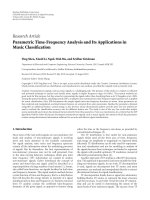
Figure 2: The surface of the time-lag kernel at the location of half maximum for (a) the GT- and (b) ST-spectrogram.
a window function ψ(t) can be expressed by the extended
Cohen’s class representation

C

t, f

= F
τ → f
F
θ →t

F
−1
u
→θ

x
∗

u −
1
2
τ

x


u +
1
2
τ

·
φ

θ, τ; f


=
F
τ → f

x
∗

t −
1
2
τ

x

t +
1
2
τ


⊗
t
Φ

t, τ; f


,
(24)
with the kernel function
φ
(ST)

θ, τ; f

=
e
−jπτθ

Ψ

u
f

Ψ
∗

u − θ
f


e
j2πτu
du, (25)
or the time-lag kernel function
Φ
(ST)

t, τ; f

=
f
2
ψ

f

−
t +
1
2
τ

ψ
∗

f

−
t −
1

2
τ

.
(26)
The proof can be found in the Appendix. Because
the window width of the ST is frequency dependent, the
corresponding kernel functions also depend on frequency.
The time-lag kernel function in Theorem 1 canhelpus
understand the locally stationary areas defined by the ST-
spectrogram. For example, the window function of the ST
originally proposed by Stockwell [9] is a Gaussian function,
that is, ψ
(ST)
(t) = (1/
√
2π)e
−t
2
/2
. This is because the
Gaussian function provides an optimal joint time-frequency
resolution. The corresponding kernel function and the time-
lag kernel function can be derived from Theorem 1
φ
(ST)

θ, τ; f

=



f


2
√
π
e
−((τ
2
f
2
/4)+(π
2
θ
2
/f
2
))
,
Φ
(ST)

t, τ; f

=
f
2
2π

e
−f
2
(t
2
+τ
2
/4)
.
(27)
Note that the time-lag kernel function is the product of two
single-variable Gaussian functions
Φ
(ST)

t, τ; f

= k
1

t; f

·k
2

τ; f

=

f

√
π
e
−f
2
t
2

·

f
2
√
π
e
−f
2
τ
2
/4

,
(28)
where one is scaled by 1/(
√
2 f ) and the other by
√
2/f.We
can measure the FWHM of the Gaussians as an approxima-
tion to the size of the time-lag kernels. Figures 2(a) and 2(b)

illustrate the surface of time-lag functions at the location
of half maximum for the GT- and ST-spectrograms, respec-
tively. The locally stationary areas are frequency-invariant for
the GT-spectrogram. On the contrary, the locally stationary
area defined by the ST-spectrogram changes with respect to
frequency: wide stationary area is applied to capture low-
frequency information of the autocorrelation function, and
a narrow stationary area is used to localize high-frequency
components. Therefore, the multiscale time-varying spec-
trogram provides a robust and accurate description of the
time-varying spectral information of a locally stationary time
series.
EURASIP Journal on Advances in Signal Processing 7
4. Time-Varying Coherence Estimated by
the Stockwell Transform
In many applications, interdependence between two time
series changes over time. It is necessary to have statistical
measures such as time-varying coherence that can reveal
such a dynamic relation. In this section, we define a time-
varying coherence function for locally stationary time series
by extending the Fourier-based coherence function to the
time-frequency plane.
The generalization of time-varying coherence using the
Cohen’s class distributions follows straightforwardly the
time-varying spectrum. The time-varying cross spectrum
can be defined with the Cohen’s class distributions by
replacing the autocorrelation function in (17) with the cross-
correlation function. Based on the representation of the
Cohen’s class, the time-varying cross spectra at each time
instant can be interpreted as the spectral representation

of the local cross-correlation function, which measures the
linear interaction between the underlying two time series
at this time instant. Similarly, the time-varying coherence
function is defined as the normalization of the time-varying
cross spectrum.
The time-varying coherence certainly inherits the char-
acteristics of the time-varying spectra. Therefore, the mul-
tiscale characteristic of the ST-spectrogram makes it an
effective tool to study the time-varying coherence. The ST
cross spectrum and coherence can be defined as follows:
TS
(ST)
xy

t, f

= E

ST
x

t, f

·ST
∗
y

t, f



,
TC
(ST)

t, f

=



TS
(ST)
xy

t, f




2
TS
(ST)
xx

t, f

·TS
(ST)
yy


t, f

.
(29)
As a scale-free measure, the value of the time-varying coher-
ence is expected to range from 0 to 1. Theorem 2 indicates
that such property holds for the ST-based coherence.
Theorem 2 (range of ST coherence). Let the window function
ψ
∈ L
2
(R) and satisfy

∞
−∞
ψ(t)dt = 1. For any two signals
x(t), y(t)
∈ L
2
(R), the following inequality holds for the ST,



TS
(ST)
xy

t, f





2
≤ TS
(ST)
xx

t, f

·
TS
(ST)
yy

t, f

.
(30)
The proof follows directly the Schwartz inequality.
Hence, 0
≤ TC
(ST)
(t, f ) ≤ 1. Note that the spectrogram
defined by the STFT also satisfies this inequality. However,
for the Cohen’s class distributions with negative values,
their corresponding time-varying coherence functions do
not hold this inequality. As a result, most of bilinear TFRs are
not suitable to study the time-varying linear interdependence
of time series.
Besides the ST, the wavelet transforms also provide

a multiscale resolution. Therefore, they can be applied
to define the time-varying spectrum and coherence. The
differences between the Stockwell approach and the wavelet
approach have been investigated recently in [24].
5. Numerical Simulations
To demonstrate the performance of the ST-spectrogram in
studying the time-varying characteristic of time series, we
estimate the time-varying spectra and coherence of a pair
of synthetic nonstationary time series using both the GT-
and the ST-spectrogram with the Gaussian window. The two
nonstationary time series are constructed as the follows:
s
1
(
t
)
=
⎧
⎨
⎩
e
2πj(5t
2
+10t)
+ e
2πj(40t)
+ 
1
(
t

)
,0
≤ t ≤ 0.5s,
e
2πj(5t
2
+10t)
+ e
2πj(80t)
+ 
2
(
t
)
,0.5 <t
≤ 1s,
s
2
(
t
)
=
⎧
⎨
⎩
e
2πj(5t
2
+10t)
+ e

2πj(80t)
+ 
1
(
t
)
,0
≤ t ≤ 0.5s,
e
2πj(5t
2
+10t)
+ e
2πj(40t)
+ 
2
(
t
)
,0.5 <t
≤ 1s,
(31)
where

i
(t), i = 1, 2 are independent Gaussian noise with
zero mean and identical variance. Note that both signals
consist of the same chirp signal whose frequency linearly
increases from 10 Hz to 20 Hz, and two constant frequency
components (40 Hz and 80 Hz) occurred at different time

periods. We generate two hundred trials of data using the
Monte Carlo simulations. The sampling rate is 1000 Hz and
the total sampling duration is 1s. The time-varying spectra
and the time-varying coherence are estimated using both the
GT- and the ST-spectrograms.
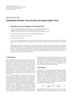
In Figure 3, the first column is the time-varying spectra
of s
1
(t); the second column is the time-varying spectra of
s
2
(t); and the third column is the coherence functions of
s
1
(t)ands
2
(t). Figures 3(a)–3(c) are the results obtained
by the GT-spectrogram with a narrower Gaussian window
(σ
= 0.05 s). The narrower time window yields a good
time resolution but a poorer frequency resolution. On the
contrary, Figures 3(d)–3(f) show the GT-based results with
a wider Gaussian window (σ
= 0.2 s), where the spectra
and the coherence function have a poorer time resolution
but a good frequency resolution. Figures 3(g)–3(i) are the
results obtained from the ST-spectrogram. The frequency-
dependent resolution produces a good time resolution at
high frequencies and a good frequency resolution at low
frequencies.

Since s
1
and s
2
are related only by the chirp signal, their
coherence should happen only at the location of the chirp
signal. Due to the limitations of the windowing technique,
the temporal occurrences of the two constant frequency
components overlap in all of the estimated time-varying
spectra, causing false coherence beyond 20 Hz around 0.5 s.
The frequency-dependent resolution of the ST-spectrogram
produces an overall better picture about the coherence of
these two signals.
6. An Application in Studying the Brain
Functional Connectivity
We now apply the time-varying coherence based on
the Stockwell transform to study functional connectivity
between the contralateral and ipsilateral motor cortices
when subjects performed the Multisource Interference Task
[25] using their right hands. The MSIT combines multiple
8 EURASIP Journal on Advances in Signal Processing
20
40
60
80
Frequency
00.20.40.60.81
Time
(a) Spectrum (Gabor) of s
1

with scale σ =
0.05 s
20
40
60
80
Frequency
00.20.40.60.81
Time
(b) Spectrum (Gabor) of s
2
with scale σ =
0.05 s
20
40
60
80
Frequency
00.20.40.60.81
Time
(c) Coherence (Gabor) with scale σ = 0.05s
20
40
60
80
Frequency
00.20.40.60.81
Time
(d) Spectrum (Gabor) of s
1

with scale σ =
0.2 s
20
40
60
80
Frequency
00.20.40.60.81
Time
(e) Spectrum (Gabor) of s
2
with scale σ =
0.2 s
20
40
60
80
Frequency
00.20.40.60.81
Time
(f) Coherence (Gabor) with scale σ = 0.2s
20
40
60
80
Frequency
00.20.40.60.81
Time
(g) Spectrum (Stockwell) of s
1

20
40
60
80
Frequency
00.20.40.60.81
Time
(h) Spectrum (Stockwell) of s
2
20
40
60
80
Frequency
00.20.40.60.81
Time
(i) Coherence (Stockwell)
Figure 3: Time-varying spectra of s
1
and s
2
and their coherence obtained from (a)–(c) the GT-spectrogram with the standard derivation of
the Gaussian window σ
= 0.05 s, (d)–(f) the GT-spectrogram with the standard derivation of the Gaussian window σ = 0.2 s, and (g)–(i)
the ST-spectrogram.
dimensions of cognitive interference in a single task, which
can be used to investigate mental or behavioral diseases
such as Attention Deficit Hyperactivity Disorder (ADHD)
in clinical studies [1]; see Figure 4 for details of the MSIT.
Fifty interference trials were recorded for two right-handed

participants (SB and DM, represented by their initials). One
hundred fifty-one channel whole-head MEG (sample rate
=
625 Hz) was recorded continuously for 400 seconds. Time
zero is represented as a press of the button. The signals at
contralateral and ipsilateral motor cortices were extracted
using the beamformer technique [26] and filtered with a low-
pass filter (1–30 Hz). Several preprocessing steps have been
applied to the data, including temporal normalization to give
the data equal weight and ensemble mean subtraction to
remove first-order nonstationarity [27].
For each subject, we calculate the time-varying spectrum
based on the ST-spectrogram with the preprocessed data
−1–1.5 s. To investigate the statistical significance of time-
varying coherence measure, we apply the bootstrap method
[28] with 500 resamples and significance level α
= 0.01.
Since the Stockwell time-frequency representation often
contains artifacts at the two ends of a time series due to
circular Fourier spectrum shifting in the implementation,
we examine the significant ST-based time-varying coherence
EURASIP Journal on Advances in Signal Processing 9
Interference trial example
0.5s 3s 0.5s
+ 322
1
2
3
Task: “ Which one of these numbers is
not like the others ? ”

In this example, the 3 is different than
the 2 s, so push button 3. Note that for
interference trials, the targets never
match the button location, and the
flanker stimuli are always potential
targets. Thus, stimuli are
relatively difficult to perform.
Correct response
Total set of possible interference stimuli:
{313, 212, 331, 221, 233, 332, 112, 211, 311,
131, 322, 232}.
Figure 4: An illustration of the multisource interference task.
5
10
15
20
25
30
Frequency
−0.6 −0.5 −0.4 −0.3 −0.2 −0.10
Time
(a) Significant time-varying coherence (Stockwell) of the subject DM
5
10
15
20
25
30
Frequency
−0.6 −0.5 −0.4 −0.3 −0.2 −0.10

Time
(b) Significant time-varying coherence (Stockwell) of the subject SB
Figure 5: The significant time-varying coherence based on the ST-
spectrogram for the subjects DM and SB.
only during the time period −0.6–0 s. Another reason why we
are particularly interested in this period is that the reaction
time of those two subjects is approximately 0.6 s, which
suggests that subjects are processing their cognitive tasks
within the time interval.
The ST-based coherence indicates the functional connec-
tion between the MIc and MIi under the MIST. Figure 5
shows that the significant connection happens mainly
around frequency bands of 10–14 Hz and 25 Hz. For the
10–14 Hz frequency band, our results are consistent with
the results found in [29], where activities of MIi and
predominantly corticocortical coupling around 8–12 Hz
have been observed under the unimanual auditorily paced
finger-tapping task. The connection around 25 Hz in this
experiment is new and needs to be further investigated.
The common limitation of studying brain signals is the
unavailability of large amounts of data. Statistical measure-
ments with few samples may combine with artifacts. In order
to improve accuracy, grand average results among more
subjects need to be studied and will be further considered
in the future.
7. Conclusions
In this paper, we investigate the estimation of the time-
varying spectrum and the time-varying coherence for the
locally stationary time series using the Cohen’s class dis-
tributions. We have shown that the estimation of time-

varying spectrum via Cohen’s class distributions (17)is
naturally coincided with the definition of the locally sta-
tionary time series (10). In addition, the availability of the
Cohen’s class representation provides a new perspective into
the characteristics of time-varying spectrum via studying
the properties of the corresponding kernel. However, to
maintain physical meaningness in time-varying spectrum
and coherence, only nonnegative Cohen’s class distribution
is preferable. To more accurately capture the local features
of a locally stationary time series, a distribution with a
multiscale resolution is desirable although most of the
standard Cohen’s class distribution have fixed resolution.
Therefore, we propose new time-varying measures based on
the spectrogram of the Stockwell transform, a hybrid of the
Short-time Fourier transform and the wavelet transform.
We prove that as a bilinear TFR, the ST-spectrogram is
a Cohen’s class distributions with a frequency-dependent
kernel. The multiscale analysis and the nonnegativity feature
make the ST an effective approach to investigate the time-
varying characteristics of the spectrum and the interaction of
10 EURASIP Journal on Advances in Signal Processing
locally stationary time series. We successfully apply the ST-
based time-varying coherence to study the brain functional
connectivity in an MEG study.
Appendix
A. Proof of Theorem 1
Consider the spectrogram of the Stockwell transform
ST

t, f


·ST
∗

t, f

=
f
2

∞
−∞
x
(
τ
)
ψ

f
(
τ − t
)

x
∗
(
τ

)
ψ

∗

f
(
τ

−t
)

e
−j2π(τ−τ

) f
dτ dτ

.
Let τ
= u +
1
2
v,andτ

= u −
1
2
v
= f
2

∞

−∞
x

u +
1
2
v

x
∗

u −
1
2
v

ψ

f

u +
1
2
v
−t

ψ
∗

f


u −
1
2
v
−t

e
−j2πvf
dv du
= F
v → f

x

t +
1
2
v

x
∗

t −
1
2
v

⊗
t


f
2
ψ

f

−
t +
1
2
v

ψ
∗

f

−
t −
1
2
v

=
F
v → f

x


t +
1
2
v

x
∗

t −
1
2
v

⊗
t
Φ
(ST)

t, v; f


.
(A.1)
Then, the kernel function can be obtained as
φ
(ST)

θ, v; f

=

F
−1
t
→θ

Φ
(ST)

t, v; f


=
f
2
F
−1
t
→θ

ψ

f

−
t +
1
2
v

ψ

∗

f

−
t −
1
2
v

=
f
2

F
−1
t
→θ

ψ

f

−
t +
1
2
v

⊗

θ

F
−1
t
→θ

ψ
∗

f

−
t −
1
2
v

=

e
jπvθ
Ψ

θ
f

⊗
θ


e
−jπvθ
Ψ
∗

−
θ
f

=

Ψ

u
f

Ψ
∗

u − θ
f

e
jπv(2u−θ)
du
= e
−jπvθ

Ψ


u
f

Ψ
∗

u − θ
f

e
j2πvu
du.
(A.2)
The interchange of the order of integrals is guaranteed
by the Fubini’s theorem since the window function ψ(t)is
bounded and ψ(t)
∈ L
2
(R).
Acknowledgments
The authors would like to thank the financial support
from Natural Sciences and Engineering Research Council of
Canada and Ontario Centres of Excellence.
References
[1] G. Bush, T. J. Spencer, J. Holmes et al., “Functional mag-
netic resonance imaging of methylphenidate and placebo
in attention-deficit/hyperactivity disorder during the multi-
source interference task,” Archives of General Psychiatry, vol.
65, no. 1, pp. 102–114, 2008.
[2] G. Buzsaki, Rhythms of the Brain,OxfordUniversityPress,

New York, NY, USA, 2006.
[3]S.L.MarpleJr.,Digital Spectral Analysis with Applications,
Prentice Hall, Englewood Cliffs, NJ, USA, 1987.
[4] M. B. Priestley, “Evolutionary spectra and non-stationary
processess,” Journal of the Royal Statistical Society: Series B, vol.
27, no. 2, pp. 204–237, 1965.
[5] L. Cohen, Time-Frequency Analysis, Prentice Hall, Englewood
Cliffs, NJ, USA, 1995.
[6] M. B. Priestley, Spectral Analysis and Time Series, vol. 2,
Academic Press, New York, NY, USA, 1981.
[7] S. Adak, Time-dependent spectral analysis of nonstationary time
series, Ph.D. thesis, Stanford Univerisity, 1996.
[8] I. Daubechies, Ten Lectures on Wav ele ts, SIAM, Philadelphia,
Pa, USA, 1992.
[9] R. G. Stockwell, L. Mansinha, and R. P. Lowe, “Localization of
the complex spectrum: the S transform,” IEEE Transactions on
Signal Processing, vol. 44, no. 4, pp. 998–1001, 1996.
[10] H. Zhu, B. G. Goodyear, M. L. Lauzon et al., “A new local
multiscale Fourier analysis for medical imaging,” Medical
Physics, vol. 30, no. 6, pp. 1134–1141, 2003.
[11]B.G.Goodyear,H.Zhu,R.A.Brown,andJ.R.Mitchell,
“Removal of phase artifacts from fMRI data using a Stockwell
transform filter improves brain activity detection,” Magnetic
Resonance in Medicine, vol. 51, no. 1, pp. 16–21, 2004.
[12] C. R. Pinnegar, “Polarization analysis and polarization fil-
tering of three-component signals with the time-frequency S
transform,” Geophysical Journal International, vol. 165, no. 2,
pp. 596–606, 2006.
[13] A. M. Yaglom, An Introduction to the Theory of Stationary
Random Functions, Prentice Hall, Englewood Cliffs, NJ, USA,

1962.
[14] R. A. Silverman, “Locally Stationary Random Processes,” IRE
Transactions on Information Theory, vol. 3, pp. 182–187, 1957.
[15] R. A. Hedges and B. W. Suter, “Improved radon-transform-
based method to quantify local stationarity,” in Advanced Sig-
nal Processing Algorithms, Architectures, and Implementations
X, F. T. Luk, Ed., vol. 4116 of Proceedings of SPIE, pp. 17–24,
San Diego, Calif, USA, August 2000.
[16] R. A. Hedges and B. W. Suter, “Numerical spread: quantifying
local stationarity,” DigitalSignalProcessing,vol.12,no.4,pp.
628–643, 2002.
[17] L. Galleani, L. Cohen, and B. Suter, “Locally stationary noise
and random processes,” in Proceedings of the 5th International
Workshop on Information Optics, pp. 514–519, Toledo, Spain,
June 2006.
[18] L. Galleani, L. Cohen, and B. Suter, “Local stationarity and
time-frequency distributions,” in Advanced Signal Processing
Algorithms, Architectures, and Implementations XVI, vol. 6313
of Proceedings of SPIE, San Diego, Calif, USA, August 2006.
EURASIP Journal on Advances in Signal Processing 11
[19] S. Mallat, G. Papanicolaou, and Z. Zhang, “Adaptive covari-
ance estimation of locally stationary processes,” Annals of
Statistics, vol. 26, no. 1, pp. 1–47, 1998.
[20] D. Gabor, “Theory of communication,” Journal I.E.E., vol. 93,
pp. 429–457, 1946.
[21] C. H. Page, “Instantaneous power spectra,” Journal of Applied
Physics, vol. 23, no. 1, pp. 103–106, 1952.
[22] H. Choi and W. J. Williams, “Improved time-frequency
representation of multicomponent signals using exponential
kernels,” IEEE Transactions on Acoustics, Speech, and Signal

Processing, vol. 37, no. 6, pp. 862–871, 1989.
[23] E. Wigner, “On the quantum correction for thermodynamic
equilibrium,” Physical Review, vol. 40, no. 5, pp. 749–759,
1932.
[24] C. Liu, W. Gaetz, and H. Zhu, “The Stockwell transform
in studying the dynamics of brain functions,” in Proceedings
of the International Workshop Pseudo-Differential Operators:
Complex Analysis and Partial Differential Equations, pp. 277–
291, August 2008.
[25] G. Bush and L. M. Shin, “The multi-source interference task:
an fMRI task that reliably activates the cingulo-frontal-parietal
cognitive/attention network,” Nature Protocols, vol. 1, no. 1,
pp. 308–313, 2006.
[26] D. Cheyne, A. C. Bostan, W. Gaetz, and E. W. Pang,
“Event-related beamforming: a robust method for presurgical
functional mapping using MEG,” Clinical Neurophysiology,
vol. 118, no. 8, pp. 1691–1704, 2007.
[27]M.Ding,S.L.Bressler,W.Yang,andH.Liang,“Short-
window spectral analysis of cortical event-related potentials
by adaptive multivariate autoregressive modeling: data pre-
processing, model validation, and variability assessment,”
Biological Cybernetics, vol. 83, no. 1, pp. 35–45, 2000.
[28] B. Efron, The Jackknife, the Bootstrap, and other Resampling
Plans, SIAM, Philadelphia, Pa, USA, 1987.
[29] B. Pollok, J. Gross, K. M
¨
uller, G. Aschersleben, and A.
Schnitzler, “The cerebral oscillatory network associated with
auditorily paced finger movements,” NeuroImage, vol. 24, no.
3, pp. 646–655, 2005.