Báo cáo sinh học: " Research Article Time-Frequency Based Channel Estimation for High-Mobility OFDM Systems—Part II: Cooperative Relaying Case" pptx

Hindawi Publishing Corporation
EURASIP Journal on Advances in Signal Processing
Volume 2010, Article ID 973286, 7 pages
doi:10.1155/2010/973286
Research Article
Time-Frequency Based Channel Estimat ion for High-Mobility
OFDM Systems—Part II: Cooperative Relaying Case
Erol
¨
Onen, Niyazi Odabas¸io
˘
glu, and Aydın Akan (EURASIP Member)
Department of Electrical and Electronics Engineering, Istanbul University, Avcilar, 34320 Istanbul, Turkey
Correspondence should be addressed to Aydın Akan,
Received 17 February 2010; Accepted 14 May 2010
Academic Editor: Lutfiye Durak
Copyright © 2010 Erol
¨
Onen et al. This is an open access article distributed under the Creative Commons Attribution License,
which permits unrestricted use, distribution, and reproduction in any medium, provided the original work is properly cited.
We consider the estimation of time-varying channels for Cooperative Orthogonal Frequency Division Multiplexing (CO-OFDM)
systems. In the next generation mobile wireless communication systems, significant Doppler frequency shifts are expected the
channel frequency response to vary in time. A time-invariant channel is assumed during the transmission of a symbol in the
previous studies on CO-OFDM systems, which is not valid in high mobility cases. Estimation of channel parameters is required at
the receiver to improve the performance of the system. We estimate the model parameters of the channel from a time-frequency
representation of the received signal. We present two approaches for the CO-OFDM channel estimation problem where in the first
approach, individual channels are estimated at the relay and destination whereas in the second one, the cascaded source-relay-
destination channel is estimated at the destination. Simulation results show that the individual channel estimation approach has
better performance in terms of MSE and BER; however it has higher computational cost compared to the cascaded approach.
1. Introduction
In wireless communication, antenna diversity is intensively

used to mitigate fading effects in the recent years. This
technique promises significant diversity gain. However due
to the size and power limitations of some mobile terminals,
antenna diversity may not be practical in some cases (e.g.,
Wireless Sensor Networks). Cooperative communication [1–
3], also referred to as cooperative relaying, has become a
popular solution for such cases since it maintains virtual
antenna array without utilizing multiple antennas. Single-
carrier modulation schemes are usually used in cooperative
communication in the case of the flat fading channel [3].
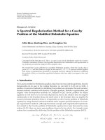
A simple cooperative communication system with a source
(S), a relay (R), and a destination (D) terminal is shown in
Figure 1.
In beyond third generation and fourth generation wire-
less communication systems, fast moving terminals and
scatterers are expected to cause the channel to become
frequency selective. Orthogonal Frequency Division Multi-
plexing (OFDM) is a powerful solution for such channels.
OFDM has a relatively longer symbol duration than single-
carrier systems which makes it very immune to fast channel
fading and impulsive noise. However, the overall system
performance may be improved by combining the advantages
of cooperative communication and OFDM systems (CO-
OFDM) when the source terminal has the above-mentioned
physical limitations
As in the traditional mobile OFDM systems, large fluctu-
ations of the channel parameters are expected between and
during OFDM symbols in CO-OFDM systems, especially
when the terminals are mobile. To combat this problem,
accurate modeling and estimation of time-varying channels

are required. Early channel estimation methods for CO-
OFDM assume a time-invariant model for the channel
during the transmission of an OFDM symbol, which is not
valid for fast-varying environments [4, 5].
A widely used channel model is a linear time-invariant
impulse response where the coefficients are complex Gaus-
sian random variables [5]. In this work we present channel
estimation techniques for CO-OFDM systems over time-
varying channels. We use the parametric channel model
2 EURASIP Journal on Advances in Signal Processing
Destination terminalSource terminal
Relay terminal
R
DS
h
SR
h
RD
h
SRD
h
SD
Figure 1: A simple cooperative communication system.
[6] employed in MIMO-OFDM system discussed in Part
I. We consider two different scenarios similar to [7]: (i)
h
SR
is estimated at the relay, and h
RD
is estimated at the

destination individually; (ii) the cascaded channel of h
SR
and
h
RD
, that is, the equivalent channel impulse response h
SRD
is
estimated at the destination terminal. Here h
SR
denotes the
channel response between S and R, h
RD
denotes the channel
response between R and D,andh
SRD
is the equivalent
cascaded channel response between S and D. Since no
channel estimation is performed at the relay, this approach
has the advantage in terms of computational requirement
over the first one.
We will show here that the parameters of these individual
as well as the cascaded time-varying channels can be
obtained by means of time-frequency representations of the
channel outputs.
The rest of the paper is organized as follows. In Section 2,
we give a brief summary of the parametric channel model
and CO-OFDM signal model. Section 3 presents time-
frequency channel estimation for CO-OFDM systems via
DET. In Section 4, we present computer simulations to

illustrate the performance of proposed channel estimation in
both scenarios mentioned above. Conclusions are drawn in
Section 5.
2. CO-OFDM System Model
2.1. Time-Varying CO-OFDM Channel Model. In this paper,
all channels are assumed multipath, fading with long-
term path loss, and Doppler frequency shifts. Path loss is
proportional to d
−a
where d is the propagation distance
between transmitter and receiver, and a is the path loss
coefficient [8]. Let G
SR
= (d
SD
/d
SR
)
a
and G
RD
= (d
SD
/d
RD
)
a
are defined as relative gain factors of (S → R)and(R → D)
links relative to (S
→ D) link [7, 9]. Here, d

SD
, d
SR
,andd
RD
denote the distances of (S → D), (S → R), and (R → D)
links, respectively.
In this study, we use the same time-varying channel
model given in Section 2.2 of Part I of this series. We
show here that the channel parameters between source-to-
destination (S
→ D), source-to-relay (S → R), relay-to-
destination (R
→ D) and the cascaded channel, and source-
to-relay-to-destination (S
→ R → D) may all be estimated
through the spreading function of the channels. Let the
channel (S
→ D)begivenby
h
SD
(
m, 
)
=
L
SD
−1

i=0

λ
i
e
jθ
i
m
δ
(
 −D
i
)
. (1)
The spreading function corresponding to h
SD
(m, )is
obtained by taking the Fourier transform with respect to m
as
S
SD
(
Ω
s
, 
)
=
L
SD
−1

i=0

λ
i
δ
(
Ω
s
−θ
i
)
δ
(
k
−D
i
)
,(2)
where L
SD
is the number of transmission paths, θ
i
represents
the Doppler frequency shift, λ
i
is the relative attenuation,
and D
i
is the delay in path i.Inbeyond3Gwireless
mobile communication systems, Doppler frequency shifts
become significant and have to be taken into account.
The spreading function S

SD
(Ω
s
, ) displays peaks located
at the time-frequency positions determined by the delays
and the corresponding Doppler frequencies, with λ
i
as their
amplitudes. In this study, we extract the individual as well
as the cascaded channel information from the spreading
function of the received signals at the relay and at the
destination.
The cascaded source-to-relay-to-destination (S
→ R →
D) channel may be represented in terms of the individual
channels as follows. Let the (S
→ R) and the (R → D)
channels be given by
h
SR
(
m, 
)
=
L
SR
−1

i=0
α

i
e
jψ
i
m
δ
(
 −N
i
)
,
h
RD
(
m, 
)
=
L
RD
−1

i=0
β
i
e
jϕ
i
m
δ
(

 −M
i
)
.
(3)
The equivalent impulse response of the cascaded (S
→ R →
D) channel may be obtained as follows:
h
SRD
(
m, 
)
= h
SR
(
m, 
)
 h
RD
(
m, 
)
=

r
h
SR
(
m, r

)
h
RD
(
m, 
−r
)
=

r
L
SR
−1

i=0
α
i
e
jψ
i
m
δ
(
r − N
i
)
×
L
RD
−1


q=0
β
q
e
jϕ
q
m
δ

 −r −M
q

=
L
SR
−1

i=0
α
i
e
jψ
i
m
L
RD
−1

q=0

β
q
e
jϕ
q
m
δ

 −N
i
−M
q

=
L
SR
−1

i=0
L
RD
−1

q=0
α
i
β
q
e
j(ψ

i
+ϕ
q
)m
δ

 −N
i
−M
q

,
(4)
where  stands for convolution. After defining the parame-
ters L
SRD
= L
SR
L
RD
, z = iL
RD
+ q, γ
z
= α
i
+ β
q
, ξ
z

= ψ
i
+ ϕ
q
,
EURASIP Journal on Advances in Signal Processing 3
and Q
z
= N
i
+ M
q
, we obtain the impulse response of the
cascaded (S
→ R → D) channel as
h
SRD
(
m, 
)
=
L
SRD
−1

z=0
γ
z
e
jξ

z
δ
(
 −Q
z
)
. (5)
In our second approach, instead of estimating the individual
channel parameters, we obtain the equivalent γ
z
, ξ
z
,andQ
z
parameters.
2.2. CO-OFDM Signal Model. We consider an Amplify-
and-Forward (AF) cooperative transmission model where a
source sends information to a destination with the assistance
of a relay [3, 10]. In this model, all of the terminals are
equipped with only one transmit and one receive antenna.
To manage cooperative transmission, we consider a special
protocol which is originally proposed in [10] and named
“Protocol II”. According to this protocol, total transmission
is divided in two phases. In Phase I, source sends OFDM
signal to both relay and destination terminals. Relay terminal
amplifies the received signal in the same phase. In Phase
II, relay terminal transmits the amplified signal to the
destination terminal.
The OFDM symbol transmitted from the source at Phase
Iisgivenby

s
(
m
)
=
1
√
K
K−1

k=0
X
k
e
jω
k
m
,(6)
where m
=−L
CP
, −L
CP
+1, ,0, , K − 1, L
CP
is the
length of the cyclic prefix, and N
= K + L
CP
is the total

length of one OFDM symbol. The received signals at relay
and destination suffer from time and frequency dispersion
of the channels, that is, multipath propagation, fading and
Doppler frequency shifts. Thus, the received signals at the
relay and destination in Phase I are
r
R
(
m
)
=

G
SR
E
L
SR
−1

=0
h
SR
(
m, 
)
s
(
m
−
)

+ n
R
(
m
)
=

G
SR
E
1
√
K
K−1

k=0
X
k
L
SR
−1

i=0
α
i
e
jψ
i
m
e

jω
k
(m−N
i
)
+ n
R
(
m
)
,
r
D1
(
m
)
=

G
SD
E
L
SD
−1

=0
h
SD
(
m, 

)
s
(
m
−
)
+ n
D1
(
m
)
=

G
SD
E
1
√
K
K−1

k=0
X
k
L
SD
−1

i=0
α

i
e
jψ
i
m
e
jω
k
(m−N
i
)
+ n
D1
(
m
)
,
(7)
where n
R
(m)andn
D1
(m) represent the additive white
Gaussian channel noise at (S
→ R)and(R → D)
channels, respectively. Here E represents the transmitted
OFDM symbol energy. The signal r
R
(m)isamplifiedbya
factor 1/


E[r
R

2
] at the relay and then transmitted to the
destination in Phase II. The signal at the output of R
→ D
channel, received by the destination terminal, is
r
D2
(
m
)
=

G
RD
E
L
RD
−1

=0
h
RD
(
m, 
)
r

R
(
m
−
)

E


r
R

2

+ n
D2
(
m
)
. (8)
Now, using the cascaded equivalent of h
SR
(m, )and
h
RD
(m, )from(5), we get
r
D2
(
m

)
=

G
SR
G
RD
E
2
E
[
r
R

2
]
⎛
⎝
L
SRD
−1

z=0
h
SRD
(
m, z
)
s
(

m
−
)
+n

R
(
m
)
⎞
⎠
+ n
D2
(
m
)
=

G
SR
G
RD
E
2
E
[
r
R

2

]
×
⎛
⎝
1
√
K
L
SRD
−1

z=0
K
−1

k=0
γ
z
e
jξ
z
m
e
jω
k
(m−Q
z
)
+ n


R
(
m
)
⎞
⎠
+ n
D2
(
m
)
,(9)
where n

R
(m) is the response of the (R → D) channel to the
n
R
(m)noise
n

R
(
m
)
=
L
RD
−1


=0
h
RD
(
m, 
)
n
R
(
m
−
)
. (10)
The receiver at the destination terminal discards the cyclic
prefix and demodulates the received signals r
D1
(m)and
r
D2
(m) using a K-point DFTs. For example the demodulated
signal corresponding to r
D1
(m)is
R
D1
k
=
1
√
K

K−1

m=0
r
D1
(
m
)
e
−jω
k
m
=
1
K
⎛
⎝
K−1

m=0
K
−1

s=0
X
s
L
SD
−1


i=0
λ
i
e
jθ
i
m
e
jω
s
(m−D
i
)
⎞
⎠
e
−jω
k
m
+N
D1
k
=
1
K
K−1

s=0
X
s

L
SD
−1

i=0
λ
i
e
−jω
s
D
i
K−1

m=0
e
jθ
i
m
e
j(ω
s
−ω
k
)m
+ N
D1
k
.
(11)

If the Doppler shifts in all S
→ D channel paths are
negligible, θ
i
≈ 0, for all i, then the channel is almost time-
invariant within one OFDM symbol, and
R
D1
k
= X
k
L
SD
−1

i=0
λ
i
e
−jω
k
D
i
+ N
D1
k
= X
k
H
k

+ N
D1
k
,
(12)
where H
SDk
is the frequency response of the almost time-
invariant channel and N
D1
k
is the DFT of the r
D1
(m).
By estimating the channel frequency response coefficients
H
SDk
, data symbols, X
k
, can be recovered according to (12).
Estimation of the channel coefficients is usually achieved by
using training symbols P
k
, called pilots inserted between data
symbols. Then the transfer function is interpolated from the
4 EURASIP Journal on Advances in Signal Processing
responses to P
k
by using different filtering techniques. This is
called Pilot Symbol Assisted (PSA) channel estimation [11].

However, in beyond 3G communication systems, fast
moving terminals and scatterers are expected in the envi-
ronment, causing the Doppler frequency shifts to become
significant which makes the above assumption invalid. In
this paper, we consider a completely time-varying model
for the CO-OFDM channels where the parameters may
change during one transmit symbol [12], based on the time-
frequency approach.
3. Time-Varying Channel Estimation for
CO-OFDM Systems
In this section we consider the estimation procedure of time-
varying CO-OFDM channels (S
→ R), (R → D)aswell
as the cascaded (S
→ R → D) channels. We approach the
channel estimation problem from a time-frequency point of
view and employ the channel estimation technique proposed
in Part I of this series. Details on the Discrete Evolutionary
Transform (DET) that we use here as a time-frequency
representation of time-varying CO-OFDM channels may be
found in Section 3 of Part I.
The time-varying frequency response or equivalently the
spreading function of the individual as well as the cascaded
channels may be calculated by means of the DET of the
received signal.
We consider two channel estimation approaches for the
CO-OFDM system illustrated in Figure 1.
3.1. Individual Channel Estimation Approach. The (S
→
R) channel is estimated at the relay terminal, then the

transmitted signal is amplified, and new pilot symbols are
inserted for the estimation of (R
→ D) channel. The pilot
symbols that are inserted at the source are effected by the
multipath fading nature of the (S
→ R) channel, as such
may not be used for the estimation of (R
→ D) channel.
Therefore, we need to insert fresh pilot symbols and extend
the length of the OFDM symbol at the relay. The estimated
(S
→ R) channel information is quantized and transmitted
to the destination together with the data symbols. Then at
the destination terminal, the (R
→ D) channel is estimated
and used for the detection. Parameters of both h
SR
(m, )and
h
RD
(m, ) channel impulse responses are estimated according
to the procedure explained in Section 3 of Part I.
3.2. Cascaded Channel Estimation Approach. The relay ter-
minal does not perform any channel estimation. The cas-
caded (S
→ R → D) channel is estimated at the destination
terminal.
The received signal r
D2
(m)canbegiveninmatrixform

as
r
= Ax, (13)
where
r
=
[
r
D2
(
0
)
, r
D2
(
1
)
, , r
D2
(
K
−1
)
]
T
,
x
=
[
X

0
, X
1
, , X
K−1
]
T
,
A
=

a
m,k

K×K
, a
m,k
=
H
SRD
(
m, ω
k
)
e
jω
k
m
√
K

.
(14)
We ignore the additive noise in the sequel to simplify the
equations. If the time-varying frequency response of the
channel H
SRD
(m, ω
k
) is known, then X
k
may be estimated by
x = A
−1
r. (15)
Calculating the DET of r
D2
(m), we get
r
D2
(
m
)
=
K−1

k=0
R
D2
(
m, ω

k
)
e
jω
k
m
,
=
1
√
K
K−1

k=0
H
SRD
(
m, ω
k
)
X
k
e
jω
k
m
,
(16)
where R
D2

(m, ω
k
) is the time-varying kernel of the DET
transform. Comparing the above representations of r
D2
(m),
we require that the kernel is
R
D2
(
m, ω
k
)
=
1
√
K
L
SRD
−1

i=0
γ
i
e
jξ
i
m
e
−jω

k
Q
i
X
k
. (17)
Finally, the time-varying channel frequency response for the
nth OFDM symbol can be obtained as
H
SRD
(
m, ω
k
)
=
√
KR
D2
(
m, ω
k
)
X
k
. (18)
Calculation of R
D2
(m, ω
k
)insuchawaythatitsatisfies(17)

is explained in Section 3 of Part I by using windows that are
adapted to the Doppler frequencies.
According to the above equation, we need the input
pilot symbols P
k
to estimate the channel frequency response.
Here we consider simple, uniform pilot patterns; however
improved patterns may be employed as well [11].
Equation (18) can be given in matrix form as
H
=
√
KRX
−1
, (19)
where
H 

h
m,k

K×K
, h
m,k
= H
SRD
(
m, ω
k
)

,
R 

r
m,k

K×K
, r
m,k
= R
D2
(
m, ω
k
)
,
X  Ix,
(20)
EURASIP Journal on Advances in Signal Processing 5
where I denotes a K
× K identity matrix. The above relation
is also valid at the preassigned pilot positions k
= k

H

SRD

m, ω
p


=
H
SRD
(
m, ω
k

)
=
√
KR
D2
(
m, ω
k

)
X
k

, (21)
where p
= 1, 2 , P and H

SRD
(m, ω
p
)isadecimatedversion
of the H

SRD
(m, ω
k
). Note that P is again the number of pilots,
and d
= K/P is the distance between adjacent pilots. Taking
the inverse DFT of H

SRD
(m, ω
p
)withrespecttoω
p
and
DFT with respect to m, we obtain the subsampled spreading
function S

SRD
(Ω
s
, )
S

SRD
(
Ω
s
, 
)
=

1
d
L
SRD
−1

i=0
γ
i
δ
(
Ω
s
−ξ
i
)
δ

 −Q
i
d

. (22)
Note that, the evolutionary kernel R
D2
(m, ω
k
)canbecal-
culated directly from r
D2

(m), and all unknown channel
parameters can be estimated according to (21)and(22)for
a time-varying model that does not require any stationarity
assumption. Estimated channel parameters are used for
the detection at the destination terminal according to the
channel equalization algorithm presented in Section 3.2 of
Part I.
In the following, we demonstrate the time-frequency
channel estimation as well as the detection performance of
our approach by means of examples.
4. Experimental Results
In our simulations, a CO-OFDM system scenario with a
source, a relay, and a destination terminal is considered
with the following parameters: the distances d
SR
and d
RD
are chosen such that the relative gain ratio G
SR
/G
RD
takes
the values
{−40, 0,40}dB, where the path loss coefficient
is assumed to be a
= 2[7]. The angle between S → R
and R
→ D propagation paths is taken as θ = 2π/3.
The performance of both individual and cascaded channel
estimation approaches is investigated by means of the mean

square error (MSE) and the bit error rate (BER) according
to varying signal-to-noise ratios. QPSK-coded data symbols
X
k
are modulated onto K = 128 subcarriers to generate
one OFDM symbol. 16 equally spaced pilot symbols are
inserted into OFDM symbols. The S
→ R, R → D,
and S
→ D channels are simulated randomly. For each
of these channels, the maximum number of paths is set
to L
= 5 where the delays and the attenuations on each
path are chosen as independent, normal distributed random
variables. Normalized Doppler frequency on each path is
fixed to f
D
= 0.2[12].
The channel output is corrupted by zero-mean AWGN
whose SNR is changed between 0 and 35 dB.
(1) Individual Channel Estimation Results. The S
→
R and R → D channels are estimated at the
corresponding terminals and are available at the
destination. Moreover, the S
→ D channel is
estimated at the destination by using the signal
r
D1
(m). Then data symbols are detected from the

0 5 101520253035
10
−3
10
−2
10
−1
MSE
SNR (dB)
Individual, 40 dB
Individual,
−40 dB
Individual, 0 dB
(a)
0 5 101520253035
10
−5
10
−4
10
−3
10
−2
10
−1
BER
SNR (dB)
Individual, 40 dB
Individual,
−40 dB

Individual, 0 dB
Perfect CSI
(b)
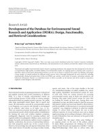
Figure 2: Performance of the individual channel estimation
approach. (a) MSE versus SNR, (b) BER performance versus SNR.
received signals r
D1
(m)andr
D2
(m) by using this
channel information. Figure 2(a) shows the total
MSE of the channel estimations S
→ R and R → D
for G
SR
/G
RD
={−40, 0,40} in dB. We see that we
obtain the best channel estimation for 0 dB which
corresponds to equal distance between S
→ R and
R
→ D. We give the BER performances at different
channel noise levels for G
SR
/G
RD
={−40,0, 40}dB
in Figure 2(b). We also compare and present our
results with the performance of the perfect channel

state information (CSI) in the same figure. Similar
to the MSE, we have the closest BER performance
to the perfect CSI for the case of G
SR
/G
RD
= 0dB.
We observe from this figure that, the “individual
approach for 0 dB” has about 5 dB SNR gain over the
“individual 40 dB” at BER
= 10
−4
.
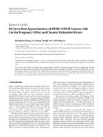
(2) Cascaded Channel Estimation Results: The combined
S
→ R → D channel is estimated at the destination
terminal from r
D2
(m). The S → D channel is esti-
mated at the destination by using the signal r
D1
(m).
Data symbols are detected from r
D1
(m)andr
D2
(m)
by using estimated channel parameters. Figure 3(a)
6 EURASIP Journal on Advances in Signal Processing
5101520253035

10
−2
10
−1
10
0
MSE
SNR (dB)
Cascaded, 40 dB
Cascaded,
−40 dB
Cascaded, 0 dB
(a)
0 5 101520253035
10
−4
10
−2
10
0
BER
SNR (dB)
Cascaded, 40 dB
Cascaded,
−40 dB
Cascaded, 0 dB
Perfect CSI
(b)
Figure 3: Performance of the cascaded channel estimation
approach. (a) Change in the MSE by SNR, (b) BER versus SNR.

shows the MSE of the cascaded S → R → D channel
estimation for G
SR
/G
RD
={−40,0, 40}dB. Note that
we obtain almost the same estimation performance
for
−40 and 40 dB and obtain better results for
G
SR
/G
RD
= 0dB as in the individual channel
estimation case. We show the BER performance for
G
SR
/G
RD
={−40, 0,40}dB,aswellasfortheperfect
CSI case in Figure 3(b). The noise floors in the figures
are due to the fact that we do not consider advanced
detection techniques for the receiver in our studies.
Our main concern is the estimation of the time-
varying channel. By using more advanced detection
methods, error floors shown in our figures may be
reduced.
Notice that the individual channel estimation approach
outperforms the cascaded approach in terms of both
MSE and BER as expected, at the expense of twice the

computational complexity. This comes from the fact that
relay terminal estimates the channel and transmits to the
destination with an increased symbol duration due to
the insertion of new pilot symbols. In approach two, the
5 10152025 3035
10
−3
10
−2
10
−1
10
0
MSE
SNR (dB)
Cascade, 8 pilot
Cascade, 16 pilot
Cascade, 32 pilot
Individual, 8 pilot
Individual, 16 pilot
Individual, 32 pilot
(a)
0 5 10 15 20 25 30 35
10
−5
10
−4
10
−3
10

−2
10
−1
BER
SNR (dB)
Cascade, 8 pilot
Cascade, 16 pilot
Cascade, 32 pilot
Individual, 8 pilot
Individual, 16 pilot
Individual, 32 pilot
(b)
Figure 4: Effect of the number of pilots in both approaches. (a)
Change of MSE by SNR, (b) change of BER by SNR.
relay does not perform any channel estimation; hence the
computational burden is reduced. However, the estimated
combined channel parameters are not as reliable as in the first
approach.
We have also investigated the effect of the number
of pilots to the channel estimation performance in both
approaches. We show the BER and MSE plots in Figures
4(a) and 4(b),respectively,forP
={8, 16,32}.Notice
that increasing the number of pilots improves the BER
performance in both approaches especially the cascaded
approach.
The effect of the number of channel paths on the BER
is illustrated by a simulation where the number of pilots is
taken as P
={8, 16} and the SNR = 15 dB. The number of

EURASIP Journal on Advances in Signal Processing 7
3 5 7 9 11 13 15 17 19 21 23 25
10
−3
10
−2
10
−1
10
0
10
1
BER
Number of paths (SNR = 15 dB)
Cascade, 8 pilot
Cascade, 16 pilot
Individual, 8 pilot
Individual, 16 pilot
Figure 5: BER performance change by the number of channel paths
for 8 and 16 pilots, and 15 dB SNR.
paths is changed between 3 and 25, and the BER is presented
in Figure 5. Note that both approaches equally suffer from
increasing the number of paths.
5. Conclusions
In this paper, we present a time-varying channel estima-
tion technique for CO-OFDM systems. We propose two
approaches where in the first one, individual channels are
estimated at the relay and destination whereas in the second
approach, the cascaded source-relay-destination channel is
estimated at the destination. We assume that the communi-

cation channels are multipath and affected by considerable
Doppler frequencies. Simulation results show that the indi-
vidual channel estimation approach gives better performance
than the cascaded approach in terms of both estimation
error and the bit error rate. However, in the cascaded
channel estimation case, the computational cost is reduced
significantly at the expense of decreased performance. We
observe that the best performance is achieved when the
distances of source-to-relay and relay-to-destination is equal,
for both approaches.
Acknowledgment
This work was supported by The Research Fund of The
University of Istanbul, project nos. 6904, 2875, and 6687.
References
[1] A. Sendonaris, E. Erkip, and B. Aazhang, “User cooperation
diversity—part I: system description,” IEEE Transactions on
Communications, vol. 51, no. 11, pp. 1927–1938, 2003.
[2] A. Sendonaris, E. Erkip, and B. Aazhang, “User cooperation
diversity—part II: implementation aspects and performance
analysis,” IEEE Transactions on Communications, vol. 51, no.
11, pp. 1939–1948, 2003.
[3] J.N.Laneman,D.N.C.Tse,andG.W.Wornell,“Cooperative
diversity in wireless networks: efficient protocols and outage
behavior,” IEEE Transactions on Information Theory, vol. 50,
no. 12, pp. 3062–3080, 2004.
[4] H. Do
ˇ
gan, “Maximum a posteriori channel estimation for
cooperative diversity orthogonal frequency-division multi-
plexing systems in amplify-and-forward mode,” IET Commu-

nications, vol. 3, no. 4, pp. 501–511, 2009.
[5] Z. Zhang, W. Zhang, and C. Tellambura, “Cooperative OFDM
channel estimation in the presence of frequency offsets,” IEEE
Transactions on Vehicular Technology, vol. 58, no. 7, pp. 3447–
3459, 2009.
[6] P. A. Bello, “Characterization of randomly time-variant linear
channels,” IEEE Transactions on Communication Systems, vol.
11, pp. 360–393, 1963.
[7] O. Amin, B. Gedik, and M. Uysal, “Channel estimation for
amplify-and-forward relaying: Cascaded against disintegrated
estimators,” IET Communications, vol. 4, no. 10, pp. 1207–
1216, 2010.
[8] J. W. Mark and W. Zhuang, Wireless Communication and
Networking, Prentice Hall, Upper Saddle River, NJ, USA, 2003.
[9] H. Ochiai, P. Mitran, and V. Tarokh, “Variable-rate two-
phase collaborative communication protocols for wireless
networks,” IEEE Transactions on Information Theory, vol. 52,
no. 9, pp. 4299–4313, 2006.
[10] R. U. Nabar, H. B
¨
olcskei, and F. W. Kneub
¨
uhler, “Fading relay
channels: performance limits and space-time signal design,”
IEEE Journal on Selected Areas in Communications, vol. 22, no.
6, pp. 1099–1109, 2004.
[11] S. G. Kang, Y. M. Ha, and E. K. Joo, “A comparative
investigation on channel estimation algorithms for OFDM in
mobile communications,” IEEE Transactions on Broadcasting,
vol. 49, no. 2, pp. 142–149, 2003.

[12] Z. Tang, R. C. Cannizzaro, G. Leus, and P. Banelli, “Pilot-
assisted time-varying channel estimation for OFDM systems,”
IEEE Transactions on Signal Processing, vol. 55, no. 5, pp. 2226–
2238, 2007.