Báo cáo hóa học: " Research Article Field Division Routing" potx

Hindawi Publishing Corporation
EURASIP Journal on Wireless Communications and Networking
Volume 2010, Article ID 560797, 17 pages
doi:10.1155/2010/560797
Research Article
Field Division Routing
Milenko Drini
´
c,
1
Darko Kirovski,
1
Lin Yuan,
2
Gang Qu,
3
and Miodrag Potkonjak
4
1
Microsoft Research, One Microsoft Way, Redmond, WA 98052, USA
2
Synopsys, 700 East Middlefield Road, Mountain View, CA 94043, USA
3
University of Maryland, 1417 A. V. Williams, College Park, MD 20742, USA
4
Computer Science Department, UCLA, B oelter Hall 3532G, Los Angeles, WA 90095, USA
Correspondence should be addressed to Milenko Drini
´
c,
Received 15 December 2009; Revised 15 April 2010; Accepted 17 June 2010
Academic Editor: Athanasios V. Vasilakos

Copyright © 2010 Milenko Drini
´
c et al. This is an open access article distributed under the Creative Commons Attribution
License, which permits unrestricted use, distribution, and reproduction in any medium, provided the original work is properly
cited.
Multihop communication objectives and constraints impose a set of challenging requirements that create difficult conditions for
simultaneous optimization of features such as scalability and performance. Routing in wireless multihop networks represents a
crucial component of the overall network efficacy because it is a lower layer that enables the actual functionality of networks.
We have developed field division routing (FDR), a distributed and nonhierarchical routing protocol that aims to coordinated
addressing of scalabilit y, topology alternations, latency, throughput, energy efficiency, and local storage requirements. FDR is
based upon two optimization mechanisms: a reactive and focused diffusion that collects only network topology information
directly required for making localized routing decisions, and a protocol for sharing routing information among neighboring nodes.
Routing table initialization and maintenance are scalable in terms of both storage and overhead traffic necessary for building
routing tables. FDR provides guaranteed connectivity while providing near-optimal all-node-pairs message delivery. The protocol
is also power-efficient to a wide spectrum of topology changes that induce relatively few messages to update routing tables network-
wide. We analyzed the new routing protocol both theoretically and using simulation.
1. Introduction
Wireless ad hoc networks (WAHNs) are commonly
abstracted as a system of application-specific devices (nodes)
with processing, storage, communication, and often sensing
capabilities where nodes communicate via radio frequency
waves. The communication range is often substantially
shorter than the network diameter. Therefore, each node
acts as a router and communicates with other nodes via
a multi-hop protocol. Routing protocols in WAHNs play
an important role as they have ramifications on the key
system requirements: (i) scalability, (ii) resilience to topology
change, (iii) overall node connectiv ity, communication (iv)
latency (delay) and (v) throughput, (vi) power consumption,
and (vii) local storage requirements [1].Theroleofrouting

in WAHNs is to enable primary functionality of a network
such as monitoring of objects, detection of different type
of events, and data distribution and dissemination with
a purpose for actuation on observed events. Due to its
importance, routing in WAHNs has been addressed in
numerous proposals that target various subsets of the
seven criteria. Nevertheless, due to the complex set of often
contradictory requirements, the search for ever improving
protocols continues.
Routing decisions in WAHNs are supported either using
routing tables that specify the network topology or using a
geographic routing criterion for making localized forwarding
decisions (see Section 2). The first class of protocols requires
hard-to-scale worldwide routing table updates upon each
topology change, while guaranteed message delivery (see
Figure 1) and shortest-path communication are the key
challenges for the latter class.
A popular heuristic approach that addresses criteria (iii–
vi) is to ensure shortest-path routing between any two
nodes in the network that can potentially communicate
while minimizing the storage requirement at each node.
All-shortest-paths routing is difficult to achieve using a
scalable distributed protocol in the presence of arbitrary
2 EURASIP Journal on Wireless Communications and Networking
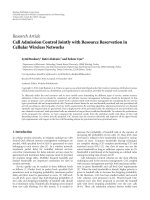
Figure 1: Challenges of multi-hop routing: In a relatively chal-
lenging setting with four disjoint communication obstacles, we
generated a fully connected network of 200 (illustrated), 500, and
1000 nodes. GPSR [2] succeeded in connecting only 79%, 88.6%,
and 90.3%, respectively, node pairs; thus, in a randomly generated
traffic model, approximately 10–20% of all trafficislikelynotto

reach destination in these networks.
topology changes. We aim for this objective and propose
a novel, distributed protocol, field division routing (FDR),
that targets all of the seven system requirements. In FDR,
each node contains all information necessary to distribute
messages to any other node in the network; each node derives
this information based upon the geographic location of a
relatively small subset of nodes, which are located in its
vicinity. Each node divides the geographical network field
into a tile of zones unique for this node. Traffictoallnodesin
one zone is routed via a neighbor uniquely assigned to that
zone. If all FDR tables are computed centrally, they enable
all-shortest-paths routing in a network with static topology
[3]. Here, we explore the more complex but significantly
more energy-efficient and scalable approach where each
node computes and maintains its own routing table in the
presence of an ever-changing network topology.
Under the mild assumption that the network is within
a finite field and that each node is aware of its geographic
location, we introduce a Discovery protocol that computes
a near-optimal shortest-paths routing table for a given node
in a relatively message-intensive manner. Since Discovery
must be repeated for each node upon every topology change,
we reduce the network maintenance overhead by introducing
a novel and near-optimal procedure for routing table
Inheritance from neighboring nodes. Next, we propose
a distributed protocol for network “initialization” with an
objective to reduce the number of nodes that perform
Discovery while computing their routing tables. In order
to support a dynamic network topology, that is, arbitrary

motion of nodes and obstacles, we introduce algorithms
for routing table “updates” that address n ode movement
that is modeled by node appearance and disappearance. The
two procedures are based upon the low-cost Inheritance
protocol. Therefore, we believe that FDR addresses the key
system requirements (i–vii) simultaneously; it is scalable,
establishes provable connectivity, is power efficient because
network dynamics initiates few messages to update routing
tables, enables near-optimal shortest-path message delivery,
and its routing tables are compact.
A shorter version of this paper with the same title has
been presented in [4]. Compared to the shorter paper, this
paper contains more detailed explanation of the underlying
FDR concepts with additional examples for better clarifica-
tion. It also contains an extended set of experimental results.
Finally, it contains proofs for all the presented theorems,
which were omitted in the previous version due to space
constraints.
2. Related Routing Protocols
Routing protocols for WAHNs can be categorized as proac-
tive, reactive, or hybrid. Each node that uses a proactive
protocol stores sufficient data about the network topology
in its routing table. Routing tables are periodically updated
such that any time a node needs to send a packet, the
forwarding route is already known and can be immediately
used [5–8]. Proactive protocols involve high overhead; size
of routing tables does not scale well with network growth
and routing table updates typically require some form of
network flooding. Also, the cost of routing table maintenance
rises with increased node mobility. One of the efforts aimed

at reduction of network flooding due to change in network
topology is Fisheye State Routing, which disseminates infor-
mation in such a way that frequent updates are limited to
node’s geographical vicinity while the frequency of updates
is reduced for nodes at larger distances [9].
In reactive protocols, a node initiates route discovery only
when it forwards a packet. Frequently used routes are cached.
Reactive protocols are suitable for highly dynamic networks
where node mobility renders the cost of proactive protocols
prohibitive [10–12]. The topology of WAHNs is closely
related to the relative positions of nodes. Geographically
assisted protocols exploit this property by making localized
decisions on forwarding routes. Greedy Perimeter Stateless
Routing (GPSR) [2] reduces the network topology to a
planar graph. It forwards messages in the direction of an
intended receiver while avoiding areas without forwarding
nodes—as a consequence, GPSR cannot guarantee successful
message delivery (see Figure 1). An extension to GPSR deals
with realistic connections that often do not correspond to
typically assumed u nit graph network representations [13].
LAR [14]andCarNet[15] use node locations and a grid
to limit the search for new routes. The main drawback of
reactive protocols is increased message latency and traffic
overheadduetoroutediscoveryforeachnoncachedroute.
Hybrid protocols leverage on the advantages of both pro-
and reactive routing schemes. Zonal protocols use proactive
routing within a zone of limited scope and reactive routing
on a global level [16, 17]. DDR divides a network into
nonoverlapping zones and uses zone identifiers to effectively
forwardmessagesbetweenzones[18]. Zonal protocols fall

into the class of hierarchical protocols since a single node
contains only limited scope information. LANMAR [19]
identifies logical subnets and assigns IP-like addresses to
them. Another important class of protocols examines the
quality of a link or multiple links in order to deliver messages
more reliably [20], with less complexity [21], or improved
performance [22].
EURASIP Journal on Wireless Communications and Networking 3
Some of the most popular current research direction for
protocols in WAHNs include techniques for identification
of connected dominating set for formation of a virtual
backbone for dissemination of updating information for
routing tables [23–25], predictive cashing strategies [26],
new variants of zonal routing [27], and exploration of
dynamic addressing techniques [28].
A related class of routing algorithms is clustering-
based protocols. In such algorithms, nodes are grouped
into clusters such that for each cluster there is an elected
node that collects, processes, and forwards data from all
the nodes within its cluster to a base station. If compared
by a routing criterion, these algorithms are similar to
zone routing algorithms. This class of routing algorithms
combines network layer with a data layer to achieve flexibility
bandwidth and resource allocation, and improved power
control. Algorithms from this class are distinguished among
each other by the way a cluster is for med and the way a
central cluster node is elected. One of the first in this class
of algorithms is Low-Energy Adaptive Clustering Hierarchy
(LEACH), which changed the premise how an elected node
in a cluster has to be fixed [29]. LEACH-C is a centralized

version of LEACH where a base station utilizes its knowledge
aboutanetworkinordertooptimizeclustersandelected
nodes [30]. Power Efficient Gathering in Sensor Information
Systems (PEGASISs) enhances collaboration among nodes
within a cluster and thus improves network operation life-
time [31, 32]. Base Station Controlled Dynamic Clustering
Protocol (BCDCP) utilizes a high-energy base station to set
up clusters and routing paths, perform randomized rotation
of cluster heads, and carry out other energy-intensive tasks
[33]. Among more recent approaches is Cluster-Chain
Routing Protocol (CCRP), which introduces adaptive power
adjustment strategy in order to take into account more
realistic wireless network connections [34].
FDR is a proactive hybrid non-hierarchical (“flat”)
protocol. In addition, FDR is fully distributed; no node
needs directions from a centralized location (base station) in
order to make routing decisions. At each node, FDR stores
and updates only information that is necessary to make
routing decisions at that node. Thus, FDR does not store or
update the entire network topology for each node, which is
required for other “flat” routing protocols. Simultaneously,
it provides each node with the ability to forward messages
to any part of the network. Size of FDR tables and update
cost is comparable to hierarchical protocols, but FDR
avoids burdening certain nodes with routing all messages
from/to their assigned zones. In addition, FDR is resilient
to irregularities of nodes’ communication radius [13, 35,
36]. Since FDR uses network topology to derive routing
tables, these irregularities affect only the shape of the routing
zones. As a key result, FDR addresses well the key system

requirements (i–vii).
3. FDR—Preliminaries
In this section, we introduce a set of assumptions and basic
definitions. First, we constrain geographically the considered
class of networks to a limited area of arbitrary shape.
We refer to this area as the “network field”. AsetofN
nodes N
={n
1
, , n
N
} is distributed within the network
field. We assume that each node is aware of its location.
This can be achieved either using a global positioning
system or a location discovery algorithm [37]. Two nodes
can communicate only if the Euclidean distance between
them is small er than their communication range and there
are no obstacles to their communication. Communicating
nodes are called “neighbors”. For brevity, we adopt that
the communication range of all nodes in the network is a
constant, r. This assumption is strict, however, the proposed
algorithms tolerate variability of r within the network as well
as for a single node over longer periods of time.
We model the dynamics of network’s topology using
two atomic events: “appearance” and “disappearance” of a
node in/from the communication range of another node.
Using these two events, we model node motion, creation
or destruction of a node within the network field, and
communication obstacles in motion. We do not impose any
constraints on the frequency of these events, though their

frequency may affect adversely the routing efficiency of the
system. A node moving fast within the network field may be
disconnected from the nodes in the network other than its
immediate neighbors, until it reduces speed of motion. We
adopt the Random Walk mobility model [38].
From the viewpoint of a single node n
i
, the network field
is tiled into “routing zones” Z
i
={z
i
1
, , z
i
Z
i
}.Eachsetof
routing zones is node specific. Each zone in Z
i
is a polygon of
arbitrary shape with one corner positioned at n
i
.Eachzone
in Z
i
is assigned exactly one neighbor to n
i
.Wedenote|Z
i

|
as the cardinality of the set Z
i
.
Definition 1 (Routing Neighbor). Exactly one neig hbor to n
i
is assigned to each of its routing zones. We define such a
neighbor as a routing neighbor.
Each routing zone is defined with up to two “borders”.
Each border is defined using a set of straight chain-connected
“border line segments”, whereas each border line segment
(abbr., line) connects a pair of “border points”. In the general
case, border lines could be represented using polynomials
of arbitrary degree. In order to reduce the complexity of
calculations, we adopted the border representation with a
polynomial of the first degree. A zone is defined using two
borders that originate at n
i
and intersect as a final point
the border of the network field. The field border connects
borders’ ends to form a single polygon. In a less frequent case,
a routing zone does not extend to the border of the network
field. (In our experiments, the frequency of occurrence of
such cases ranges approximately from 0.0001% to 0.001%.)
Such a case can occur in a network with large areas that
do not contain any nodes. In such case, a routing zone is
described using a sing le border w hich star t s and ends at
n
i
. Since this type of a routing zone occurs infrequently,

throughout this paper, we refer to routing zones defined
using two borders.
FDR supports two fundamental message delivery mech-
anisms: location and name based. In case a source node
n
i
knows the geographic location of the message recipient
4 EURASIP Journal on Wireless Communications and Networking
Figure 2: An example of a network field divided into three routing
zones for node s. Each zone is assigned to respective neighbor nodes
a, b,andc of s. Routing zones are defined using points x
1
, x
2
, x
3
,
and x
4
.
n
j
, it finds the routing zone that contains n
j
and sends
the message to the routing neighbor assigned to that zone.
Here, we assume that all traffic in the network conforms
to this model. FDR can be adjusted to support name-based
message delivery as well. Next, the source node must first
discover the geographic position of the destination node and

then forward the message using the location-based delivery
process. There are several simple protocols that can be used
to announce the position of a node to the remainder of the
network. Detailed analysis of name-based message delivery
protocols is beyond the scope of this paper.
An example of a WAHN is shown in Figure 2.We
consider the routing zones built from the viewpoint of
node s.Nodes divides the network field into three routing
zones. These zones are assigned to neighboring nodes a,
b,andc. The neighboring node a is assig ned to the
routing zone described with borders
{(s, x
1
), (x
1
, x
2
)},and
{(s, x
3
)}. The neighboring node b is assigned to the routing
zone described with borders
{(s, x
3
)} and {(s, x
4
)}.The
neighboring node c is assigned to the routing zone described
with borders
{(s, x

4
)} and {(s, x
1
), (x
1
, x
2
)}.Fulldescription
of each routing zone includes the border of the network.
We assume that each node knows the defining points of the
enclosing network field: y
1
, y
2
, y
3
,andy
4
. Thus, the routing
table for each node contains only information about the
tiling of the network field into zones.
4. Routing Table Initialization
In this section, we describe how nodes initialize their routing
tables using FDR. During initialization, each node divides
the network field into routing zones and assigns a routing
neighbor to each routing zone. The construction process
relies on several key observations related to network topology
and connectivity.
Definition 2 (Essential Node). If the shortest path from a
source node n

i
to a destination node n
j
leads exclusively via
one neighbor n
k
of n
i
, then n
j
is a node essential to n
i
.
s
a
1
a
2
a
3
b
1
b
2
b
3
b
4
d
2

d
3
Figure 3: An example of a network used to demonstrate why a
network field is divided by essential nodes.
Definition 3 (Esse ntial Neighbor). Let n
j
be an essential node
to n
i
. A neighbor n
k
of n
i
, which is the first hop on the
shortest path from n
i
to n
j
, is referred to as an “essential
neighbor” of n
i
.
Consider the example in Figure 3.Nodes is the source.
Then, nodes a
2
and a
3
are essential nodes because the
shortest path to these nodes leads only via node a
1

. Similarly,
b
2
, b
3
,andb
4
are essential nodes since the shortest path from
s to any of them leads only via b
1
.Nodesa
1
and b
1
are
essential neighbors of s.
To achieve shortest-path routing, a message from a
source node toward any essential node must be routed only
via other essential nodes of the source. Consider the node b
3
in the example in Figure 3. All messages from s to b
3
have b
1
as their first hop. Note that b
3
is not an essential node of b
1
because two shortest paths from b
1

to b
3
exist via b
2
and b
4
,
respectively.However,bothb
2
and b
4
are essential nodes to s.
We formulate the above statements more formally.
Theorem 4. The shortest path from a source node s toward any
essent ial node routed via the same neighbor n leads only via
nodes that are essential to s. (Proofs of all theorems are included
in the appendix.)
Theorem 5. The shortest path from a source node s toward any
nonessent ial node leads only via nonessential nodes.
4.1. Selection of Routing Neighbors. When a source node
is building its FDR table, it has to determine how many
zones will divide the network field (
|Z
i
|) and select the
corresponding routing neighbors. The key observation of
this paper is that this process can be performed locally in
a deterministic fashion. This means that any node in the
field can determine the number of its routing zones by only
observing the topology of its local neighborhood. Here we

present the proof for this claim.
EURASIP Journal on Wireless Communications and Networking 5
Based on Theorem 4, we know that the shortest path to
all essential nodes leads only via essential nodes.
Corollary 6. From Theorem 4, it follow s that if there is an
essential node e at distance α hops from a source node s,where
α>2, there exists an essential node at distance 2 from s via
which the shortest path leads to e.
Corollary 7. From Theorem 5, it follows that if there is a
nonessential node n at distance β from a source node s,where
β>2, then there exists a noness ential node at distance 2 from s
via which the shortest path leads to n.
From Corollaries 6 and 7, it follows that a node can deter-
mine which of its neighbors are essential and nonessential
by observing the network topology at a distance of two hops
from itself. In other words, a node can which the necessary
of routing zones is necessary to cover the entire network by
only observing neighboring network topology at distance of
2 hops from itself. This topology can be easily obtained for
each node in a network if each node broadcasts a list of its
neighbors.
We describe this process using an example in Figure 3.
Node s broadcasts a message to its neighbors requesting that
they send the list of their neighbors. Node a
1
returns a list
with nodes a
2
and d
2

,andb
1
returns a list with nodes b
2
, b
4
,
and d
2
.Nodes concludes that a
2
is only covered by node a
1
and therefore it is essential. Similarly, nodes b
2
and b
4
are
essential, while node d
2
is covered by both neighbors. We
denote d
2
adon’t-care node. In this case, both neighbors are
essential. Thus, s creates two routing zones with nodes a
1
and
b
1
assigned to each zone. A source node selects all essential

neighbors and a subset of nonessential neighbors as routing
neighbors such that all nodes in the network are covered.
Definition 8 (Don’t-care Node). A node that can be assigned
to either routing zone with preserved shortest path routing is
a “don’t-care node”.
Algorithm 1 outlines the algorithm that identifies essen-
tial and nonessential neighbors and selects routing neigh-
bors. The goal of the algorithm presented in Algorithm 1
is to select as few as possible nonessential neighbors that
are assigned to routing zones. Since each routing neigh-
bor corresponds to one routing zone, by minimizing this
number, we heuristically aim at reducing the number of
stored borders, that is, the storage requirement, at each node.
This problem can be reduced to the constrained minimum
sequence covering problem (CMSC), which is NP-hard [39].
CMSC can be defined as fol lows.
Problem. Constrained minimum sequence covering.
Instance. A finite sequence of symbols D
={d
1
, d
2
, , d
n
};a
set of templates T
={t
1
, t
2

, , t
k
} such that each template t
i
is formed by concatenating an arbitrary number of symbols
from D;sequenceS formed by concatenation of symbols
from D and integer I.
Question. Can S be covered by I instances of T such that no
two templates overlap and I is minimized.
Select Routing Neighbors
Input: source node n
i
,setT
i
of neighbors of n
i
Output: set of routing neighbors R
i
1. n
i
requests lists L(i, k)ofneighborsfromalln
k
∈ T
i
2. All n
k
∈ T
i
return L(i, k); L
i

= L
i
∪ L(i, k)
3. for each node x
l
∈ L
i
4. if x
l
appears in exactly one list L(i, j)
5. then x
l
is an essential node,
mark n
j
as an essential neighbor
6. add
all essential neighbors to R
i
7. Mark all nodes covered by neighbors already in R
i
8. while there are unmarked nodes
9. add
to R
i
a nonessential neighbor n
j
that
covers the largest number of unmarked nodes
10. mark all nodes covered by n

j
Algorithm 1: Procedure that selects and assigns neighbors to
routing zones.
If we consider node to correspond to a symbol, node
connectivity to correspond to a concatenation of symbols
into a sequence, and a selection of a neighbor that covers
certain number of nodes to correspond to a template that
covers the corresponding sequence of symbols, our problem
is reduced to CMSC. To address this problem, we propose a
particularly fast, but greedy heuristic. Note that the heuristic
may not return an optimal solution in this context, however,
in the next phase of building node’s routing table, shortest-
paths routing to all destinations can still be achieved.
4.2. Nodes Sufficient to Build a Border. The geography of
a routing zone is dependent upon the positioning of the
encompassed essential nodes. In the remainder of this paper,
we refer to all nodes covered exclusively by a single routing
neighbor as “essential nodes”. Nodes covered by more than
one routing neighbor are referred to as “don’t-care nodes”.
In both cases, for node n
k
to “cover” node n
j
from the
perspective of a source node n
i
means that n
k
is on the
shortestpathfromn

i
to n
j
. If a source node identifies all
essential nodes, it can identify all routing zones to achieve
shortest-paths routing. Unfortunately, in order to identify
all essential nodes, it appears that the source has to flood
the network. As this cost is prohibitive, we propose a more
effective solution.
In order to build borders between zones, it is not
necessary for a source node to have knowledge of the
entire network topology. Consider the example network in
Figure 4.Sourcenodes needs to build a border between two
routing zones assigned to nodes a
1
and b
1
(a border line that
originates in s). Let us assume that s has two lists of nodes: (i)
a
2
and a
3
; and (ii) b
2
and b
3
. The nodes in the lists represent
nodes that are the closest to the border between zones. They
are sufficient to completely describe the border. Node s can

ignore the positions and connections of all other essential
nodes on either side of the border while constructing it.
We now present FDR’s Discovery protocol that identi-
fies nodes necessary to build a border between two zones.
6 EURASIP Journal on Wireless Communications and Networking
s
a
3
a
2
a
1
b
3
b
2
b
1
d
3
d
2
Figure 4: An example of a network used to demonst rate why it is
sufficient to select only a subset of all essential nodes for the process
of building borders.
The key idea behind this protocol is to send two messages
along each side of the border. The messages carry the hop
count from the source and a border side identifier (i.e., coun-
terclockwise (CCW) or clockwise (CW)). This information
enables nodes along the border to identify if they are essential

or “don’t-care” nodes from source’s perspective. Source node
s uses geogr a phical location of routing neighbors pairs to
determine which one carries CW and which one CCW type
of a message. Note that in cases when s has only two routing
neighbors (such as for node s in Figure 4), only two borders
are created. When creating one border, the first neighbor is
on CW side, the second one is on CCW side. When creating
the other border, routing neighboring nodes switch roles so
the first neighbor is on CCW side, and the second one is on
CW side. We demonstrate the protocol using an exemplary
network in Figure 4.Sourcenodes identifies that a
1
and
b
1
are its essential neighbors and sends a message to a
1
and b
1
requesting a list of essential nodes along each side
of the border. In the message, s states that the border is in
the CW direction for a
1
and CCW direction for b
1
with s
as a reference node. It also states that node d
2
is a “don’t-
care” node. Node a

1
identifies a
2
as the closest node to the
border with a hop count of 2, while b
1
identifies b
2
. They
further request from a
2
and b
2
to return a list of nodes along
the border. This request includes s as a reference node and
respective orientations. Nodes a
1
and b
1
inform d
2
thatitis
a“don’t-care”nodewithahopcountof2;d
2
announces this
information to all its neighbors. Next, node b
2
identifies and
notifies b
3

as the node closest to the border (in the CCW
direction) with a hop count of 3; b
3
acknowledges that it
is at the end of the network field and returns a list to b
2
that contains node b
3
.Next,b
2
appends itself to the list and
sends it back to b
1
,andb
1
sends a list containing b
2
and
b
3
to s. On the other hand, a
2
identifies and notifies d
3
as
the one closest to the border (in the CW direction) with a
hop count of 3; d
3
receives the broadcast message from d
2

that d
2
is a “don’t-care” node with a hop count of 2. Next, it
receives the message from a
2
stating that its hop count from
the source node is 3. Since there exists a path via d
2
with a
hop count of 3, d
3
concludes that it is a “don’t-care” node.
Discovery
Input: current node x
i
, number of hops

h
Output: list of essential nodes L
i
from x
i
to
the end of network field
1. if x
i
is don’t-care
2. x
i
announces it is don’t-care to all its neighbors

3. return empty L
i
4. if x
i
is at the end of the network field
5. return L
i
= x
i
6. Sort neighbors of x
i
, {n
1
, , n
k
}, into a list N
i
,
7.theclosestnodetotheborderisattheheadofN
i
8. for each neighbor n
j
∈ N
i
9. L
i
= call Discovery(n
j
,


h +1)
10. if L
i
/
= empty
11. prepend x
i
to L
i
,thatis,L
i
= x
i
L
i
11. return L
i
12. return empty L
i
Algorithm 2: Pseudocode for FDR’s discovery protocol.
It announces this information to all its neighbors. Similar to
b
2
, a
2
identifies and notifies a
3
as the closest to the border in
the CW direction that is not “don’t-care”. Soon, it receives a
list from a

3
that contains one node, a
3
; a
2
appends itself to
the list, sends it back to a
1
,anda
1
sends the list containing
a
2
and a
3
to s.Nodes receives the list that contains nodes a
2
and a
3
on one side of the border, and b
2
and b
3
on the other
side of the border.
The Pseudocode for FDR’s Discovery protocol is pre-
sented in Algorithm 2. We present only a part of the
algorithm initiated by source’s neighbors. This part of the
algorithm is recursive. Each node can receive two types of
messages from their neighbors: a don’t-care announcement

and a request for the list of essential nodes along the
border. When a request for the list is received, node x
i
first
determines if it is a don’t-care node. This can happen if x
i
already received a don’t-care announcement with smaller or
equal hop count, or if it received another request from the
opposite side of the border with the same hop count. In
such a case, x
i
announces to its neighbors that it is a don’t-
care node. Otherwise, x
i
sorts its neighbors such that the
closest node to the border is at the head of the sorted list.
Since the border is not placed yet, x
i
uses the reference point
and a direction (CCW or CW) to determine the ordering.
Then, x
i
recursively requests the list of essential nodes from
its neighbors in the sorted order. The bottom of this recursive
procedure is when the end of the network field is reached.
Pseudocode in Algorithm 2 is presented in the form of a
function that handles the requests for the list of essential
nodes a long the border. The function returns a list that is
empty if a node is a don’t-care node.
In order to determine zones’ borders, we must identify

all nodes along the border up to the point when a border
intersects with network’s boundary. A node recognizes such
a situation when its communication range is intersecting
with this boundary. In that case, the node bottoms the
recursive procedure by performing the step 5 in Algorithm 2.
EURASIP Journal on Wireless Communications and Networking 7
Each node, when added to the network, is informed about
its boundary. We do not make any assumptions about the
shape of the finite network field. In our tests, we assumed a
rectangular field.
Discovery attempts to find all nodes necessary for
creation of zones’ borders. Due to the fact that this algorithm
is localized, sometimes it can produce borders where shortest
path routing is not preserved. We formalize this observation
in the following Theorem.
Theorem 9. Discovery can yield suboptimal results in terms
of shortest path routing.
Although Discovery can produce suboptimal results,
it is important to note that the connectivity of nodes is
preserved. This fact is very important for guarantied message
delivery.
Theorem 10. Discovery maintains node connectivity.
An important property of any routing scheme is its ability
to forward messages without cyclic paths. Cyclic paths can
result in buffer overflows, excessive energy bill, and dead
locks; clearly, the y contribute to the overall inefficiency of the
network.
Theorem 11. FDR is an acyclic routing scheme.
4.3. Building Borders. The source node initiates the pro-
cedure for building borders upon receipt of the two lists

of essential nodes (CW and CCW from the border) from
the associated pair of routing neighbors. The goal of this
procedureistocreateachainofborderlinesegments
that separates two routing zones such that node motion is
maximally tolerated. This is accomplished by placing the
border equidistantly from closest essential n odes in each
zone. We describe this procedure using an example in
Figure 5. The source node s considers essential nodes a
2
, a
3
,
a
4
,anda
5
along one side of the border (CW) and b
2
, b
3
,and
b
4
along the other (CCW). Node s uses one pointer for both
received lists. By iteratively advancing these pointers, s builds
the border. The construction process involves the following
steps:
(i) Set pointers

p

CW
= a
2
and

p
CCW
= b
2
to the
corresponding beginning of each list; set the reference
point
r = s; compute the initial minimal angle

θ =
∠(

p
CW
, r,

p
CCW
)—atfirst

θ>0.
(ii) Iteratively advance both pointers and record minimal

θ and corresponding


p
CW
and

p
CCW
; repeat until θ ≤
0. This situation occurs after advancing

p
CW
from a
3
to a
4
.
(iii) Insert the first border point c
1
at half distance from
the previous valid pointers a
3
and b
3
where

θ =
∠(a
3
, r, b
3

) > 0; set the reference point r = c
1
;
compute

θ; Reset pointers

p
CW
= a
3
and

p
CCW
= b
3
.
(iv) Iteratively advance both pointers until ends of both
lists are reached, that is,

p
CW
= a
5
and

p
CCW
= b

4
.
s
a
3
a
2
a
1
b
3
b
2
b
1
d
3
d
2
Figure 5: A network example that illustrates the procedure for
building borders.
(v) Insert the last border point c
2
at half-distance from
the current pointers a
5
and b
4
.
The Pseudocode of this procedure is shown in

Algorithm 3. The procedure does not attempt to insert
the minimal number of border points in order to address the
(vii) criterion. We have opted for a strategy where a border
point is inserted equidistantly between two conflicting
pointers. This enables less frequent updates of borders since
changes in node positions have the least effect on borders.
As most of the borders are composed of only a single border
point, the overall increase in the average routing table size is
negligible.
4.4. Routing Table Inheritance. Messages sent throughout
the network with a pur pose to discover its topology and
establish routing tables at specific nodes are considered a
routing overhead. In order to reduce this overhead, we
propose an Inheritance protocol that builds a routing table
at a single node by analyzing the already computed routing
tables of the node’s neighbors. In most cases, routing zones
of two routing neighbors overlap, that is, at least at one
location their zones’ borders intersect. The overlapping area
contains nodes that can be routed via either of the two
routing neighbors. It is necessary to determine how to divide
that area to preserve near-optimal shortest path routing
in the expected case. The proposed Inheritance protocol
estimates the required hop counts along the intersecting
borders to determine equidistant points between them. We
consider these points as border points of the new border.
Thus, the border is constructed as an estimate based upon
neighbor’s routing tables and the assumption that nodes are
placed with unifor m probability within the network field. In
case this probability map is non-uniform but relatively static
(e.g., topology of a city), the algorithm can be adjusted to this

case in a straightforward manner.
8 EURASIP Journal on Wireless Communications and Networking
BuildBorders
Input: L
CCW
and L
CW
—lists of essential nodes,

p
CCW
and

p
CW
—node pointers, source node s
Output: C—list of border points
1. Set reference point
r = s
2. Set

p
CCW
and

p
CW
to the node closest to s in
L
CCW

and L
CW
,respectively
3. Last valid pair of pointers
{V
1
, V
2
}={

p
CCW
,

p
CW
}
4. Compute

θ = ∠(

p
CW
, r,

p
CCW
)
5. repeat
6. if



p
CCW
− r < 

p
CW
− r advance

p
CCW
7. else advance

p
CW
8. Compute θ = ∠(

p
CW
, r,

p
CCW
)
9. if θ<0
10. add
point c
i
to C, c

i
is on the line V
1
, V
2
and c
i
− V
1
=c
i
− V
2

11. Place border between r and c
i
;setr = c
i
;
12.

θ = ∠(V
1
, r, V
2
); {

p
CCW
,


p
CW
}={V
1
, V
2
}
13. else if θ<

θ
14.

θ = θ; {V
1
, V
2
}={

p
CCW
,

p
CW
}
15. until both

p
CCW

and

p
CW
reach ends
of L
CCW
and L
CW
,respectively
Algorithm 3: Pseudocode of the procedure that builds borders
between two routing zones of a source node. Operator
a − b
returns the Euclidean distance between two points a and b.
s
a
1
b
1
A
1
(5)
A
2
(10)
(7)
(9)
B
1
(7)

B
2
(9)
(5)
Figure 6: An example of border placement between two routing
zones of a source node based on the routing zones of source’s
routing neighbors.
We use the example in Figure 6 to describe the Inher-
itance protocol. Assume that nodes a
1
and b
1
are routing
neighbors of a source node s,botha
1
and b
1
have already
determined their routing tables via the Discovery protocol.
Here, we make an assumption that the routing table for
node s contains an additional information about each border
point c
i
: φ
i
= min {h(s, V
1
), h(s, V
2
)},wherefunctionh(a, b)

returns the hop count from node a to node b and V
1
and
V
2
are essential nodes that determined the location of c
i
Inherit ance
Input: C
CCW
, C
CW
—lists of border points with the
hop count information for each point, source node s
Output: C—list of points for the inherited border
1. for each border line l
= c
i
, c
i+1
in C
CCW
and C
CW
2. insert φ
i+1
− φ
i
− 1 = P − 1 pseudo border points
p

0
= c
i
, p
1
···p
P−1
, p
P
= c
i+1
such that (∀j)p
j
∈ l
and
p
j+1
− p
j
=p
j
− p
j−1

3. for each p
j
4. compute its hop count estimate: φ
j
5. for each border point c
i

∈ C
CCW
∪ C
CW
6. if (∃p
j
)φ
j
= φ
i
and p
j
is at opposing border to c
i
7. add point t to C,wheret is on c
i
, p
j
and
c
i
− t=p
j
− t
Algorithm 4: Pseudocode of the procedure that builds a border
between routing zones of two adjacent routing neighbors of a source
node.
as in step 9 of the Pseudocode in Algorithm 3. Figure 6
illustrates the φ-parameter in parentheses next to the name
of a border point. The Inheritance protocol executes the

following simple steps:
(i) divide each intersecting border line into unit subseg-
ments; the unit length equals to
c
i+1
−c
i
/(φ
i+1
−φ
i
),
where c
i
and c
i+1
aretwoconsecutiveborderpoints;
(ii) connect each border point with a mirror point at
the other border; a mirror point of a border point
is a point with the same estimated hop count at the
opposing border line;
(iii) insert points for the new border equidistantly from
the connector lines.
These steps assume a uniform probability density func-
tion p(x, y) of nodes in the network field. In case p(x, y)
is not uniform, a new border point τ is placed such that

τ
c
a

p(x, y)dxdy =

c
b
τ
p(x, y)dxdy,wherec
a
is a point on
one border and c
b
is its corresponding mirror point. In this
case, unit segments are computed similarly, by integrating
p() over the border line. For simplicity of presentation, in
this paper we assume that p() is uniform. Pseudocode for the
Inheritance protocol is presented in Algorithm 4.
At last, we analyze two specific situations. When neigh-
bors’ two border zones do not overlap, then Inheritance
uses the procedure BuildBorders from Algorithm 3 to
build a new border in between the two nonintersecting
borders. The two lists of border points that correspond
to the nonintersecting borders are fed as the L
CCW
and
L
CW
input to BuildBorders. Finally, a node that has used
Inheritance to derive its routing table can fine-tune its
borders for destinations that are frequently contacted and are
located near the border. The fine-tuning can b e performed
by sending a test message via each of the candidate routing

neighbors. By learning the hop count that the test messages
had when reaching their destination, the source can readjust
the border between the two routing neighbors.
EURASIP Journal on Wireless Communications and Networking 9
As Discovery, Inheritance can produce zones where
shortest path routing is not preserved. This means that
some routes will have extra hops in message delivery, which
represents an undesirable overhead in communication. It
is important to st ress that such an overhead should be
minimized because in WAHN networks one of the critical
resources is typically nodes’ power consumption. Inheri-
tance does preserve connectivity (guaranteed message deliv-
ery) and acyclic routing. We formalize the above observation
in the following theorems.
Theorem 12. Inheritance can yield suboptimal results in
terms of shortest path routing.
Theorem 13. Inheritance preserves connectivity.
Theorem 14. Inheritance preserves acyclic routing.
4.5. Synchronizing the Initialization. We now present an
efficient protocol, SynchInit, for distributed and localized
network initialization that combines routing table c reation
via the Discovery and Inheritance protocols. The prereq-
uisite condition for applying Inheritance is that routing
neighbors of the source node have already initialized their
routing tables. We can assess the following optimization goal.
Knowing the network topology, select minimal number of
nodes whose routing tables are initialized via Discovery,
such that remaining nodes in the network can initialize their
routing tables via Inheritance.
Consider a network with N nodes. We form a collection S

of N sets as follows. For each node n
i
, create a set S
i
={n
i
};
then add to S
i
all nodes for which n
i
is their routing neighbor.
We can restate the optimization goal as the following. Select
a subset B of S such that each node belongs to at least one of
the selected sets and the cardinality of B,
|B| <K,whereK is
a given integer. This problem is equivalent to the minimum
set cover problem, which is NP-hard. This definition of the
problem refers to a situation where subsets can be chosen
centrally. In our case, the selection process is done in a
localized manner. To address the distr ibuted variant of this
problem, we propose an effective heuristic with emphasis on
protocol simplicity.
The key idea behind SynchInit is to overlay the network
field with a regular grid and initialize nodes closest to grid
intersections via Discovery. The remaining nodes are then
initialized v ia Inheritance if their prerequisite conditions
are satisfied. Next, if there still exist uninitialized nodes, Syn-
chInit increases the grid density and repeats the previous
two steps. These two steps can be iterated until all nodes are

initialized. Alternatively, SynchInit can repeat fixed number
of iterations and then force all uninitialized nodes to perform
Discovery to complete network initialization. We outline
the key steps of SynchInit using an exemplary network in
Figure 7.
(i) each node considers a virtual regular grid laid over
the network field; the grid is the same for all nodes in
the network; the shortest distance in the grid equals
2r;
s
a
1
a
2
a
3
a
4
a
5
b
1
b
2
b
3
b
4
c
1

c
2
Border point
θ
Figure 7: An example of an ad hoc wireless network that illustrates
the procedure for distributed and localized network initialization.
(ii) nodes closest to intersect ion points of the grid
initialize their routing table via Discovery;such
nodes are s, a
3
, b
1
, b
2
, b
3
,andd
2
;
(iii) nodes whose routing neighbors have already initial-
ized their routing tables use Inheritance to initialize
their routing tables; nodes b
4
and d
3
have routing
neighbors b
1
and b
3

,anda
3
and d
2
,respectively,
that have already initialized routing tables; routing
tables can be computed partially, when two angularly
adjacent routing neighbors compute their adequate
zones, the source can proceed with Inheritance to
compute its border;
(iv) double the grid density;
(v) out of all remaining uninitialized nodes, nodes a
1
and
a
2
are the closest to the new grid points; thus, they
initialize their routing tables via Discovery.
Remark 15. only nodes b
4
and d
2
have used Inheritance;
this is a consequence of a denser grid; here, the number of
nodes that used Inheritance is lower than in most practical
cases when the network is typically denser.
PseudocodeforthisprotocolisillustratedinAlgorithm 5.
Finally, we evaluate two key trade-offs related to Syn-
chInit. First, a denser grid causes more nodes to initiate
Discovery. Then, network initialization converges faster

at the expense of sending more messages. Second, we
initiate InheritanceQ times for each iteration of SynchInit
(steps 6 through 8). Nodes that have built routing tables
after Discovery can use their routing table to initiate
10 EURASIP Journal on Wireless Communications and Networking
SynchInit
Input: Node n, comm. range r,networkfieldF
Output: Initialized routing table of n
1. Overlay F using a regular grid G; the shortest
distance between two points in G is 2r
2. Find the closest grid point g
3. repeat R times
4. if n is the closest uninitialized node to g
and
n −g <r/2
5. return Discovery (n)
6. repeat Q times
7. if routing neighbors of n are initialized
8. returnInheritance (n)
9. Double the grid density
10. return Discovery (n)
Algorithm 5: Pseudocode for distributed initialization of a routing
table. In step 4, if there is a tie in terms of distance, nodes are ordered
clockwise north-first to break the tie. In our experiments, we limited
R
= 3andQ = 2.
Inheritance in other nodes. However, this is not feasible if
nodes have a mutual relationship of being routing neighbors
to each other. Such nodes cannot use Inheritance to build
their tables; thus, they wait until the grid density is increased

to proceed with their initialization.
5. Support for Network Dynamics
In this section, we propose protocols that can efficiently
cope with the management of nodes’ routing tables in the
case of a dynamic network topology. We do not bound the
space of possible changes in the network. FDR supports
introduction of new and failure of existing nodes and/or
obstacles to communication in the network field. It also
manages the case when both nodes and/or obstacles are
in motion. The two atomic events that can model any
of these cases are “appearance” and “disappearance” of a
node in/from the communication range of another node.
We denote these two events as “motion” events. When a
motion event occurs, certain nodes may become detached
from all but the neighboring nodes in the network because
their routing tables are nonexistent or invalid. This condition
may last until the node seizes its activity and some or all
routing tables of its neighboring nodes are updated. The
expectation for this condition is reduced by increasing the
communication radius r of each node. We assume that r is
chosen such that motion events occur relatively infrequently.
From the perspec tive of a specific source node, most of
the changes in the network do not have any impact on its
routing table. If a motion event occurs far from its routing
table’s borders, usually it does not affec t source’s routing
table. Consider an example shown in Figure 8.Ifanodeb
5
changes its position as indicated by the dashed arrow, the
routing table of s is not affected. As a network field w idens,
nodes’ routing zones become larger. For a larger routing

zone, it is less likely that an arbitrary motion event in the
b
7
b
5
b
3
b
4
b
6
b
2
b
1
a
1
a
2
a
3
d
3
d
2
s
Figure 8: An example of a WAHN that illustrates how node motion
does not affect the routing table of a distant node.
network results in an update of its borders. Changes in one
part of the network have a smaller expected effect on nodes

located far from the place where the motion event occurred.
This property enables FDR to be a highly scalable routing
scheme when dealing with network dynamics.
The fact that FDR reduces any network topology to rout-
ing zones and essential neighbors enables inherent tolerance
to small changes to the topology. If two nodes n
i
and n
j
are not essential neighbors to each other, disappearance of
n
i
from the communication range of any other node in
the network does not change the routing table of n
j
. If the
appearance of n
i
in the communication range of any node
in the network does not establish a new essential neighbor
relationship between n
i
and n
j
,itdoesnotaffec t the routing
table of n
j
. It is important that nodes observe such cases
where they do not need to update their tables. T his reduces
communication overhead. For example, in proactive routing

protocols the entire network would have to be flooded with
messages about the topology change such that routing tables
across the network can be updated. FDR enables situations
where network communication is avoided almost entirely
even if network topology has changed. We formalize this
observation in the foll owing theorem.
Theorem 16. For a given node n
i
, appearance or disappear-
anceofaneighboringnoden
j
does not affect the routing table
of n
i
if and only if n
j
is not a routing neighbor to n
i
.Wereferto
such a motion event as “unilaterally tolerable ”.
5.1. Node Appearance and Disappearance. Node appearance
is a motion event after which two nodes are able to directly
communicate. This event can occur due to introduction of
a new node in the network, node motion, or motion of
a communication obstacle. The objective for the protocol
that maintains nodes’ routing tables is to identify whether
any tables within the network require an update of their
routing rules and if yes, to perform the updates in the least
expensive fashion. The proposed protocol relies upon certain
key observations about how motion events alter the network

topology.
EURASIP Journal on Wireless Communications and Networking 11
MotionUpdate
Input: Source node n, existing routing table τ
0
of n,nodem
appears in its communication range
Output: Routing table of n
1. Exchange geographic location data with m
2. L
=SelectRoutingNeighbors(n)
3. if m
∈ L
4. Routing table τ
=Discovery(n)
5. if τ
0
/
=τ
6. for each neighbor p to n
7. e
p
= PRNG(), send {τ, e
p
} to p
8. return τ
9. return τ
0
MotionProp aga te
Input: Motion event e,sourcenoden, its neighbor m,and

their routing tables τ
0
n
and τ
m
,respectively
Output: Routing table of n
1. Node n receives
{τ
m
, e} from m
2. if m is a routing neighbor to n and
n has not yet updated its routing table due to e and
τ
m
affects at least one of the borders in τ
0
n
3. τ
1
n
=Inherit ance(n)
4. ifτ
1
n
/
=τ
0
n
then send {τ

1
n
, e} to all neighbors
5. return τ
1
n
6. return τ
0
n
Algorithm 6: Pseudocode for routing table update upon a motion
event. Function PRNG() returns a pseudorandom number.
When two nodes, n and m, establish communication
upon a motion event, each of them executes the MotionUp-
da te procedure outlined in Algorithm 6. After lear ning each
others’ geographical locations, each node computes its list
of routing neighbors as described in Algorithm 1. Note that
n includes m in its list of routing neighbors only if m is
an essential neighbor to n; otherwise, n forces the selection
process not to include m.Incasem is a routing neighbor,
it changes the network topology for n sufficiently so that
n needs to update its table via the Discovery protocol. If
there is any change to its routing table borders, n must
propagate these changes to its neighbors. Thus, n sends its
routing table to all its neighbors as well as a random number
e
p
distinct for each neighbor p. The purpose of e
p
is to
force the propagation within the network in the opposite

direction from n. A random number of sufficiently high
entropy should be distinct for this motion event with hig h
likelihood and can be used as its identifier.
Anoden that receives the propagation packet from its
neighbor m executes the MotionProp aga te procedure. It
ignores the package if m is not its routing neighbor or if
the received routing table actually does no affect any of
the borders in the existing routing table of n. Otherwise,
it recomputes its routing table based on the Inheritance
protocol. Note that only borders affected by the propagation
package are recomputed. If there are any changes to the
borders of the routing table of n,noden must propagate
these changes to its neighbors. The propagation package sent
by n includes the identifier of the original motion event.
s
a
1
b
1
A
1
(5)
A
2
(10)
(7)
(9)
B
1
(7)

B
2
(9)
(5)
Figure 9: An example of a motion event changing profoundly
the network topology and triggering the Discovery protocol for
routing table updates.
A motion event that triggers propagation is illustrated in
Figure 9. A path of length α hops connects nodes a and b,
where α>2. A new node c establishes a path between a and
b equal to two hops. Thus, both a and b are new essential
neighbors to c. Since routing tables of a and b are affected by
the appearance of c,nodec initiates Discovery at all three
involved nodes.
The main property of the updating protocols is that
Discovery is performed only by the nodes directly affected
by the motion event. In case there are any changes to
the routing tables, they are propagated using the localized
Inheritance protocol. In addition, the propagation typi-
cally occurs in the immediate neighborhood of the motion
event. Only events that profoundly change the topology of
the network (e.g., establish a ring as in Figure 9) initiate
network-wide propagation. The expectation is that motion
events in dense networks should trigger routing table updates
significantly less frequently than in sparser networks. Overly
sparse networks should experience common wide-spread
propagation, a mere necessity for maintaining network’s
fragile connectivity. Finally, protocols MotionUpda te and
MotionPropagate preserve the network connectivity and
establish acyclic routing. For brevity, we do not present these

claims formally in this version of the paper.
Node disappearance is an event dual in nature to node
appearance. The update procedure for this event is equivalent
to the protocol presented in Algorithm 6 with two key
differences. First, it is triggered by the disappearance of a
neighbor m from the communication range of a given source
node n. Second, during step 2 of MotionUpdate, n initially
tries to find another neighbor m

that can replace m and
preserve the existing routing table borders. If this cannot be
achieved, n recreates the list of routing neighbors with an aim
12 EURASIP Journal on Wireless Communications and Networking
to preserve as much as possible of the borders from the
existing routing table. This objective minimizes the number
of neighbors that propagate their routing table changes.
6. Experimental Results
In order to evaluate the performance of the generic FDR
platform, we conducted several experiments. We have
compared our approach with GPSR, as a state-of-the-art
reactive protocol. We opted for comparison with GPSR
because it provides similar support for network dynamics
as FDR although its routing algorithm differs significantly.
Comparison with proactive or hybrid routing protocols
could be done only in one of the performance dimensions
because their optimization goals are different from FDR’s
so they lack full support for network dynamics and/or they
do not offer same routing convenience for each node. We
have built a custom simulator for our FDR algorithm and
we have implemented GPSR algorithm as it is described in

[2].
First, we evaluated if all nodes are reachable. We have
established a network with obstacles as shown in Figure 1.
More specifically, we created a network field with four
obstacles in a realistic setting, that is, a skewed distribution of
nodes’ placement in the field. Then, we randomly generated
three network instances with 200, 500, and 1000 nodes
and measured the percentage of messages that reached
destination for each node-to-node coupling in case GPSR
was used as a routing mechanism. Only 79%, 88.6%, a nd
90.3% of messages, respectively, were delivered, while the
remainder had to terminate their path search due to exceeded
TTL. Most applications that require reliability pose a strong
demand for alternate routing mechanisms that guarantee
delivery. In addition, name-based messaging in WAHNs (see
Section 3) is particularly prone to failed message deliveries
as efficient name-based services commonly require reliable
communication.
Figures 10(a) and 10(b) illustrates histograms of path
lengths for all pairs of nodes for two randomly generated
networks of
{N,r}={200, 0.13}, {400, 0.088}.Ranger was
chosen so that the expected number of neighbors for each
node is approximately the same regardless of the number
of nodes in a network; we aimed at networks of similar
density and different area coverage. The benchmark for our
measurements was the result of the Dijkstra all-shortest-
path algorithm with unit weight for each connection between
nodes. We defined routing overhead as an additional number
of hops necessary for a message delivery compared to the

result given by the Dijkstra algorithm. We measured the
results of FDR computed via both the Discovery and
SynchInit protocols. Also, we computed path lengths using
the GPSR protocol excluding connections that were not
established. In Figure’s legend we recorded the mean path
length across all (in case of GPSR feasible) paths. One can
observe that Discovery found shortest paths in nearly all
cases (overhead of less than 1% and 2.5%) a nd SynchInit
produced overhead of 5.8% and 8.4% compared to GPSR’s
overhead of 9% and 23% (with all infeasible paths excluded)
for the network instances of 200 and 400 nodes, respectively.
Figure 10(c) illustrates the number of messages, M,
exchanged among all nodes during network initialization.
This is the entire initialization cost in FDR. Considered
networks are itemized in the caption of Figure 10.Two
different datasets are plotted, M for initialization via Dis-
covery only and via SynchInit as described in Section 4.
In almost all cases, we recorded improvement in traffic that
was nearly constant within 20–25%. For denser networks,
this improvement increased, for example, in our experiments
we recorded the largest improvement in excess of 60% for
{N,r}={1000, 0.13}. Note that the number of messages is
comparable to network “flooding;” however, FDR has several
important improvements with respect to other “flooding”
schemes. First, in FDR M
∼ O(N
√
N)versusO(N
2
)

for true “flooding.” Next, individual nodes do not have
to compute the shortest paths upon learning network’s
topology, that is, routing tables are computed in a distributed
fashion. This greatly reduces the complexity and memory
requirement of individual nodes. In addition, FDR’s routing
tables require nearly minimal storage which scales well with
network size [3]. Finally, FDR supports mobility mostly via
the Inheritance primitive which greatly reduces trafficfor
routing tables’ maintenance once connectivity is established
via SynchInit.
We simulated a large number of motion events. We
recorded the tr ail of messages s ent throughout a network in
order to propagate information about changes in network
topology. We used a uniform distribution to determine a
direction of each motion event. We used an exponentially
decreasing distribution function to determine the length of
each move with the maximum of 3 node communication
ranges. For each network type, we simulated 25 000 motion
events over 5 different network instances. Each motion event
can affect a routing table of a number of nodes, and one or
more routing borders within each table. The average number
of modified tables ranges from 12.3 for networks with
{N,r}={200, 0.130} to 17.8 for {N, r}={1000, 0.060}.
An example of a complete probability distribution is shown
in Figure 11.
The likelihood of a node launching the Discovery
protocol due to a motion event ranges from 45% for
networks with 200 nodes to 10% for networks with 1000
nodes. An example of such probability distribution is shown
in Figure 12. Figure 13 presents the overall improvement of

the cost (expressed in terms of the number of the exchanged
messages necessary for a network update) that is the result of
a use of the combination of Discovery and Inheritance
protocols, compared to the incurred cost if only the Dis-
covery protocol is used. The combination of the protocols
significantly reduces communication requirements, while
maintaining the property that all tables have updated routes
toward all nodes in the network.
7. Conclusion
In summary, the detailed presentation of the FDR f ramework
in this paper along with the experimental results show cases
of a multi-hop protocol that addresses efficiently the criteria
(i–vii) for WAHNs. Compared to GPSR, trafficoverhead
EURASIP Journal on Wireless Communications and Networking 13
0 5 10 15 20 25 30
10
−4
10
−3
10
−2
10
−1
Path length
Probability of occurrence
All-shortest paths (mean L) = 5.84
GPSR (mean L) = 6.64
Network N
= 200, r = 0.13
Discovery (mean L)

= 5.89
Synchinit(mean L)
= 6.18
(a)
0 1020304050607080
Path length
Probability of occurrence
All-shortest paths (mean L) = 8.77
10
−6
10
−5
10
−4
10
−3
10
−2
10
−1
Network N = 400, r = 0.088
GPSR (mean L)
= 10.76
Discovery (mean L) = 8.99
Synchinit (mean L) = 9.51
(b)
200 400 600 800 1000
0
1
2

3
4
5
6
7
×10
5
Number of nodes N
Number of messages during initialization
Full Discovery
Synchinit
Synchinit versus full Discovery
(c)
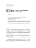
Figure 10: Probability distribution for path length in a randomly generated network N = 200, r = 0.13 (a) and N = 400, r = 0.088
(b) in a unit-square field. Number of messages sent during initialization using Discovery only and using SynchInit for three network
instances for each of the following network types:
{N, r}={200, 0.13}, {400, 0.088}, {600, 0.071}, {800, 0.061}, {1000, 0.06}. We selected
the communication range r for each network so that the expected number of neighbors for each node is approximately equivalent.
due to periodic SynchInits to optimize path lengths can be
negligible in WAHNs where nodes exchange large amounts
of data (e.g., audio/video, sensor data) and motion events
happen infrequently. Compared to other proactive schemes,
FDR offers support for node motion at low cost in overhead
traffic and requires low computational resources for nodes.
This can be particularly applicable to networks of sensors.
Throughout the paper, we used an optimization goal to
make route lengths as close as possible to the length shortest-
path routes. There exist s cenarios where such optimization
goal is not the most desirable one. Strength of wireless
signal is inversely proportional to the square distance of the

signal source so one can envision a scenario where more
hops in a message delivery can be more energy efficient
14 EURASIP Journal on Wireless Communications and Networking
s
a
1
a
2
a
3
b
1
b
2
b
3
b
4
d
2
d
3
Figure 11: Probability distribution of the number of tables and
borders affected by motion events for the network type
{N, r}=
{
600, 0.071}.
0
10 20 30
40

50 60 70 80
10
−3
10
−2
10
−1
Instances
Probabilty of occurrence
Discovery
Inheritance
Network N
= 800, r = 0.061
Figure 12: Probability distribution of Discovery protocol versus
Inherit ance protocol induced by motion events for the network
type
{N, r}={800, 0.061}.
than smaller number of hops. In our simulations, we have
neglected a possibility of noisy communication [40], need
for message retransmission, dropped connections [34], and
so forth. These realistic scenarios can certainly affect a
routing protocol. FDR is equipped with mechanisms to
handle all of the above issues, whose exploration and the
effect on FDR’s performance we leave for future work.
Other possible future directions are enhancements in FDR’s
border building algorithm where a node could cache already
explored lists of nodes that are necessary to build borders;
congestion avoidance during message routing; balancing of
power utilization for improved network lifetime.
b

7
b
5
b
3
b
4
b
6
b
2
b
1
a
1
a
2
a
3
d
3
d
2
s
Figure 13: Comparison between a system using only the Dis-
co very protocol and a system that combines the Discovery and
Inherit ance protocols.
12 34
5
23

4
s
a
1
a
5
6(5)
r
b
1
r
r
r
r/2 r/2
r/2
r/2 r/2
r/2
5(4) 6(5)12
3
4
z
yx
Figure 14: An example of a network that illustrates when Discov-
ery yields a suboptimal result. Numbers next to nodes represent the
hop count from the source node s. For nodes that have suboptimal
hop counts computed by the procedure, optimal hop counts are
given in parentheses.
Appendix
Proof of Theorem 4 (by contradiction). Assume that there
exists an essential node e at distance α from the source

node s. Next, assume that there exists a nonessential node
l at distance α
− 1froms that is connected to e. Since l is
nonessential, there exist multiple neighbors of s via which
s can forward messages to l with the smallest number of
hops. Since l is connected to e, there exist multiple neighbors
of s via which s can forward the message to e.Itfollows
that either e is not essential or there does not exist such a
nonessential node l.
EURASIP Journal on Wireless Communications and Networking 15
a
b
α>2
New node
c
Figure 15: An example of a network used to prove that FDR is
acyclic.
Proof of Theorem 5. For each nonessential node n
j
, there
exist multiple neighbors of s thatcanbeafirsthop
on the shortest path. If we remove all these neighbors
except one, all nonessential nodes become essential via the
unremoved neighbor. Lets denote all nonessential nodes
converted to essential nodes via this step as pseudoesse ntial.
We can now directly apply Theorem 4 to prove that the
shortest path toward any pseudoessential node leads via other
pseudoessential nodes.
Proof of Theorem 9 (by ex ample). Consider an example of a
network shown in Figure 14. The source node identifies

two routing zones and initiates the process of discovering
essential nodes along the border. The numbers in Figure 14
next to each node indicate the length of the shortest path
from s, while r indicates node’s communication range. The
following conditions in this example lead to incorrectly
calculating the hop count from s to x.
(i) Node a
5
has hop count of 5 from s.
(ii) The procedure discovers the subset of essential nodes
along the border and calculates the hop count of 6
from s to y.
(iii) Node z is sufficiently far from the border so the
procedure never considers it, and the hop count of
4froms to z is not calculated.
The calculated shor test path hop count from s to x is 6 (via
a
5
) while the correct hop count is 5 (via z). The procedure
then incorrectly places x in the same routing zone as A
5
.
Proof of Theorem 10. The necessary condition for Discovery
to yield suboptimal solution is that there exist two paths from
a source node to an incorrectly classified node. Even if a node
is incorrectly placed into a nother routing zone, there still
exists a routing path from the source node to that node. Thus,
a node cannot be disconnected.
Proof of Theorem 11. We consider two complementary cases;
FDR’s routing tables produce an all-shortest-paths routing;

and there exist paths that are suboptimal in terms of the
length of routing paths. In the former case, each message
deliver y between two neighboring nodes reduces the distance
to the destination node by one hop because of the shortest
path routing. Thus, a source node or any intermediate node
on the message path cannot be encountered twice, that is, the
routing is acyclic.
In the latter case, we assume that cyclic forwarding of a
message has occurred and consider two possible scenarios:
(i) there exists a pair of neighboring nodes n
i
, n
i+1
on the
forwarding path such that when n
i
sends a message to n
i+1
,
n
i+1
returns the message to n
i
, and (ii) a message returns to a
sender via a unique set of nodes (following a cyclic route).
For case (i), consider a pair of neighboring nodes n
i
and
n
i+1

. Let us assume that there exists a node x at a distance
of two hops from n
i
which is a neighbor of n
i+1
.Also,lets
assume that n
i
routes its messages to x via n
i+1
.Inorder
for n
i+1
to return message directed to x back to n
i
,ithasto
have n
i
as a first hop toward x in its routing table. However,
by the initial assumption x is a neighbor of n
i+1
so all the
messages from n
i+1
to x are sent via their direct link. Since
the procedure for selecting routing neig hbors (Algorithm 1)
considers nodes at distance of two hops, nodes n
i
and n
i+1

cannot have each other selected as first hops toward the same
node. Hence, a node cannot return a message directly to the
sender.
For case (ii), we consider a general case illustrated using
Figure 15, when FDR does not follow the shor test path
routing and shows that a cyclic routes cannot occur. Dashed
lines in Figure 15 indicate that there exists a path between
two nodes. The label on each dashed line represents the
path length. We also use this label as a name for the path.
Assume that the shortest path distance from a source s to a
destination d is α +1+β hops. Also, assume that there exists
another path between nodes a and d whose length is γ and
β<γ. At the same time, assume that β<δ+ θ<γso node
x misclassifies d to be routed via its neighbor b instead of a.
Consider a message forwarded from s to d.Afterα hops, the
message arr ives at node x, which forwards it toward d via b.
The only way for this message to enter a cycle is that at node
z, it is forwarded back on the path with κ hops toward node
c. When z builds its FDR table, it considers paths of length
θ toward d and paths κ +2+δ + θ or κ +2+γ (latter two
are cyclic via c). Node z does not consider the path of length
κ +2+β since that path has to pass via x,andx does not
consider path β as viable since it is farther from the border
than path γ. Since κ+2+δ+θ>θ<κ+2+γ
, z always chooses
the path θ for forwarding. This implies that a path cannot b e
cyclic. Note that we did not make any assumptions on path
lengths except for the conditions necessary to misclassify d in
the routing table of x.
Proof of Theorem 12 (by example). Consider an example of a

network shown in Figure 16.Nodes inherits routing tables
from nodes a
1
and b
1
. It places a new border such that
nodes a
2
and a
3
are routed via a
1
, while b
2
, b
3
,anda
4
are
routed via b
1
. Consequently, the routing path from s to a
4
increased from the minimal four hops to five hops, which is
suboptimal.
Proof of Theorem 13. From Theorem 10, it follows that all
nodes in a routing zone are reachable. When Inheritance
16 EURASIP Journal on Wireless Communications and Networking
s
b

1
b
2
b
3
a
1
a
2
a
3
a
4
d
3
d
2
A
1
(3)
(3)
Figure 16: An example of an ad hoc wireless network that illustrates
suboptimality of the Inheritance protocol.
places a node in a routing zone such that the number of
hops increases, the node has to be in the overlapping parts
of both routing zones. It follows that the node is reachable
via both neighbors of the source node from which the source
node inherited tables. Since all nodes in a routing zone
are reachable, the node is still reachable regardless of its
placement in the routing zones.

Proof of Theorem 14. Theorem 11 states that FDR features
acyclic routing. The first hop from the source node leads to
one of the neighbors from which the source node inherited
its routing table. Any of the following hops is routed via
routing tables that are not cyclic (according to Theorem 11).
Since the first hop does not cause any cyclic routing,
inherited tables preserve acyclic routing.
References
[1] E. M. Royer and C. Toh, “A review of current routing
protocols for ad hoc mobile wireless networks,” IEEE Personal
Communications, vol. 6, no. 2, pp. 46–55, 1999.
[2] B. Karp and H. T. Kung, “GPSR: greedy perimeter stateless
routing for wireless networks,” in Proceedings of the 6th Annual
International Conference on Mobile Computing and Networking
(MOBICOM ’00), pp. 243–254, August 2000.
[3] M. Drini
´
c, D. Kirovski, and M. Potkonjak, “Model-based
compression in wireless ad hoc networks,” in Proceedings of the
1st Internat ional Conference on Embedded Networked Sensor
Systems (SenSys ’03), pp. 231–242, November 2003.
[4] M. Drini
´
c, D. Kirovski, Q. Gang, L. Yuan, and M. Potkonjak,
“Field division routing,” in Proceedings of the 16th IST Mobile
and Wireless Communications Summit, July 2007.
[5] C. Perkins and P. Bhagwat, “Highly dynamic destinationse-
quenced distance-vector routing (DSDV) for mobile com-
puters,” in Proceedings of the ACM SIGCOMM Conference on
Communications Architectures, Protocols and Applications,pp.

234–244, 1994.
[6] S. Murthy and J. J. Garcia-Luna-Aceves, “A routing protocol
for packet radio networks,” in Proceedings of the 1st Annual
International Conference on Mobile Computing and Network-
ing, pp. 86–95, November 1995.
[7] P.Jacquet,P.M
¨
uhlethaler, T. Clausen, A. Laouiti, A. Qayyum,
and L. Viennot, “Optimized link state routing protocol for ad
hoc networks,” in Proceedings of the IEEE International Multi
Topic Conference, pp. 62–68, 2001.
[8] B. Bellur and R. G. Ogier, “A reliable, efficient topology broad-
cast protocol for dynamic networks,” in Proceedings of the
IEEE International Conference on Computer Communications
(INFOCOM ’99), vol. 1, pp. 178–186, 1999.
[9] G. Pei, M. Gerla, and T W. Chen, “Fisheye state routing: a
routing scheme for ad hoc wireless networks,” in Proceedings
of the IEEE International Conference on Communications, vol.
1, pp. 70–74, June 2000.
[10] Vi. D. Park and M. S. Corson, “A highly adaptive distributed
routing algorithm for mobile wireless networks,” Proceedings
of the IEEE International Conference on Computer Communi-
cations (INFOCOM ’97), vol. 3, pp. 1405–1413, 1997.
[11] D. B. Johnson and D. A. Maltz, Dynamic Source Routing in Ad
Hoc Wireless Networks, chapter 5, Kluwer Academic, Boston,
Mass, USA, 1996.
[12] C. Perkins and E. M. Royer, “Ad hoc on demand distance vec-
tor (AODV) routing,” in IEEE Wor kshop on Mobile Computing
Systems and Applications, pp. 90–100, February 1999.
[13] Y J. Kim, R. Govindan, B. Karp, and S. Shenker, “Practical

and robust geographic routing in wireless networks,” in
Proceedings of the 2nd Internat ional Conference on Embedded
Networked Sensor Systems (SenSys ’04), pp. 295–296, Novem-
ber 2004.
[14] Y B. Ko and N. H. Vaidya, “Location-aided routing (LAR) in
mobile ad hoc networks,” Wireless Networks,vol.6,no.4,pp.
307–321, 2000.
[15] R. Morris, J. Jannotti, F. Kaashoek, J. Li, and D. Decouto,
“CarNet: a scalable ad hoc w ireless network system,” in
Proceedings of the ACM SIGOPS European Workshop, pp. 61–
65, 2000.
[16] P. Samar, M. R. Pearlman, and Z. J. Haas, “Independent zone
routing: an a daptive hybrid routing framework for ad hoc
wireless networks,” IEEE/ACM Transactions on Networking,
vol. 12, no. 4, pp. 595–608, 2004.
[17] Z. J. Haas, “New routing protocol for the reconfigurable
wireless networks,” in Proceedings of the IEEE 6th International
Conference on Universal Personal Communications Record
(ICUPC ’97)
, vol. 2, pp. 562–566, October 1997.
[18] N. Nikaein and C. Bonnet, “Ddr: distributed dynamic routing
algorithm for mobile ad hoc networks,” in Proceedings of
the 1st ACM international symposium on Mobile Ad Hoc
Networking & Computing, pp. 19–27, Boston, Mass, USA,
2000.
[19] G. Pei, M. Gerla, and X. Hong, “LANMAR: landmark routing
for large scale wireless ad hoc networks with group mobility,”
in Proceedings of the Proceedings of the 1st ACM international
symposium on Mobile Ad Hoc Networking & Computing,pp.
11–18, 2000.

[20] S. Biswas and R. Morris, “Opportunistic routing in multi-
hop wireless networks,” in Proceedings of the ACM SIGCOMM
Computer Communication Review (CCR ’04), pp. 69–74, 2004.
[21] W. I. Lee and B. G. Lee, “Pre-computation based selective
probing (PCSP) scheme for distributed QoS routing,” in
Proceedings of the IEEE Global Telecommunication Conference
(GLOBECOM ’00), vol. 3, pp. 1778–1782, 2000.
[22] M. Zorzi and R. R. Rao, “Geographic random forwarding
(GeRaF) for ad hoc and sensor networks: multihop perfor-
mance,” IEEE Transactions on Mobile Computing, vol. 2, no.
4, pp. 337–348, 2003.
[23] B. Das and V. Bharghavan, “Routing in ad-hoc networks using
minimum connected dominating sets,” in Proceedings of the
IEEE International Conference on Communications (ICC ’97),
vol. 1, pp. 376–380, June 1997.
EURASIP Journal on Wireless Communications and Networking 17
[24] P. Sinha, R. Sivakumar, and V. Bharghavan, “Enhancing
ad hoc routing with dynamic virtual infrastructures,” in
Proceedings of the IEEE International Conference on Computer
Communications (INFOCOM ’01), vol. 3, pp. 1763–1772,
2001.
[25] S. Butenko, X. Cheng, D Z. Du, and P. M. Pardalos, “On
the construction of virtual backbone for ad hoc wireless
networks,” in Cooperative Control: Models, Applications and
Algorithms, vol. 1, chapter 3, pp. 43–54, Kluwer Academic,
Boston, Mass, USA, 2003.
[26] W. Lou and Y. Fang, “Predictive caching strategy for on-
demand routing protocols in wireless ad hoc networks,”
Wireless Networks, vol. 8, no. 6, pp. 671–679, 2002.
[27] P. Samar, M. R. Pearlman, and Z. J. Haas, “Independent zone

routing: an a daptive hybrid routing framework for ad hoc
wireless networks,” IEEE/ACM Transactions on Networking,
vol. 12, no. 4, pp. 595–608, 2004.
[28] J. Eriksson, M. Faloutsos, and S. Krishnamurthy, “Scalable ad
hoc routing: the case for dynamic addressing,” in Proceedings
of the 23rd Annual Joint Conference of the IEEE Computer and
Communications Societies (INFOCOM ’04), vol. 2, pp. 1108–
1119, March 2004.
[29] W. R. Heinzelman, A. Sinha, A. Wang, and A. P. Chan-
drakasan, “Energy-scalable algorithms and protocols for wire-
less microsensor networks,” in Proceedings of the IEEE Intern-
tional Conference on Acoustics, Speech, and Signal Processing,
pp. 3722–3725, June 2000.
[30] W. B. Heinzelman, A. P. Chandrakasan, and H. Balakrishnan,
“An application-specific protocol architecture for wireless
microsensor networks,” IEEE Transactions on Wireless Com-
munications, vol. 1, no. 4, pp. 660–670, 2002.
[31] S. Lindsey and C. S. Raghavendra, “PEGASIS: powerefficient
gathering in sensor information system,” in Proceedings of the
IEEE Aerospace Conference, pp. 1–6, 2002.
[32] S. Lindse y, C. S. Rag havendra, and K. M. Sivalingam, “Data
gathering algorithms in sensor networks using energy met-
rics,” IEEE Transactions on Parallel and Distributed Systems,
vol. 13, no. 9, pp. 924–935, 2002.
[33]S.D.Muruganathan,D.C.F.Ma,R.I.Bhasin,andA.O.
Fapojuwo, “A centralized energy-efficient routing protocol for
wireless sensor networks,” IEEE Communications Magazine,
vol. 43, no. 3, pp. S8–S13, 2005.
[34] X. Liu, X. Bian, and H. Cho, “A novel clusterchain channel
adaptive routing protocol in wireless sensor networks,” in

Proceedings of the International Conference on Heterogeneous
Networking for Quality, Reliability, Security and Robustness
(ICST ’08), pp. 1–7, 2008.
[35] A. Woo, T. Tong, and D. Culler, “Taming the underlying
challenges of reliable multihop routing in sensor networks,” in
Proceedings of the 1rst International Conference on Embedded
Networked Sensor Systems (SenSys ’03), pp. 14–27, November
2003.
[36] M. D. Yarvis, W. S. Conner, L. Krishnamurthy, J. Chhabr a,
B. Elliott, and A. Mainwaring, “Real-world experiences with
an interactive ad hoc sensor network,” in Proceedings of the
International Workshop on Ad Hoc Networking (IWAHN ’02) ,
pp. 143–151, 2002.
[37] J. Li, J. Jannotti, D. S. J. De Couto, D. R. Karger, and R. Morris,
“Scalable location service for geographic ad hoc routing,”
in Proceedings of the 6th Annual International Conference on
Mobile Computing and Networking (MOBICOM ’00), pp. 120–
130, August 2000.
[38] B. Liang and Z. J. Haas, “Predictive distance-based mobility
management for PCS networks,” in Proceedings of the 18th
Annual Joint Conference of the IEEE Computer and Communi-
cations Societie (INFOCOM ’99), pp. 1377–1384, March 1999.
[39] M. R. Garey and D. S. Johnson, Computers and Intractability: A
Guide to the Theory of NP-Completeness, W.H. Freeman, New
York, NY, USA, 1979.
[40] M. Z. Zamalloa, K. Seada, B. Krishnamachari, and A. Helmy,
“Efficient geographic routing over lossy links in wireless sensor
networks,”
ACM T ransactions on Sensor Networks,vol.4,no.3,
pp. 1–33, 2008.