báo cáo hóa học:" Connectivity analysis of one-dimensional vehicular ad hoc networks in fading channels" pot
Bạn đang xem bản rút gọn của tài liệu. Xem và tải ngay bản đầy đủ của tài liệu tại đây (609.46 KB, 35 trang )
1
Connectivity analysis of one-dimensional
vehicular ad hoc networks in fading
channels
Neelakantan Pattathil Chandrasekharamenon
∗
and Babu AnchareV
Department of Electronics and Communication Engineering,
National Institute of Technology, Calicut 673601, India
∗
Corresponding author: neelakantan
Email address:
AVB:
Abstract
Vehicular ad hoc network (VANET) is a type of promising application-oriented network deployed
along a highway for safety and emergency information delivery, entertainment, data collection, and
communication. In this paper, we present an analytical model to investigate the connectivity properties of
one-dimensional VANETs in the presence of channel randomness, from a queuing theoretic perspective.
Connectivity is one of the most important issues in VANETs to ensure reliable dissemination of time-
critical information. The effect of channel randomness caused by fading is incorporated into the analysis
by modeling the transmission range of each vehicle as a random variable. With exponentially distributed
inter-vehicle distances, we use an equivalent M/G/∞ queue for the connectivity analysis. Assuming
that the network consists of a large number of finite clusters, we obtain analytical expressions for the
average connectivity distance and the expected number of vehicles in a connected cluster, taking into
account the underlying wireless channel. Three different fading models are considered for the analysis:
Rayleigh, Rician and Weibull. The effect of log normal shadow fading is also analyzed. A distance-
dependent power law model is used to represent the path loss in the channel. Further, the speed of each
vehicle on the highway is assumed to be a Gaussian distributed random variable. The analytical model
is useful to assess VANET connectivity properties in a fading channel.
Keywords: connectivity distance; fading channels; highway; vehicle speed; vehicular ad hoc networks.
2
1. Introduction
Vehicular Ad Hoc Networks (VANETs), which allow vehicles to form a self-organized net-
work without the requirement of permanent infrastructures, are highly mobile wireless ad hoc
networks targeted to support (i) vehicular safety-related applications such as emergency warning
systems, collision avoidance through driver assistance, road condition warning, lane-changing
assistance and (ii) entertainment applications [1]. VANET is a hybrid wireless network that
supports both infrastructure-based and ad hoc communications. Specifically, vehicles on the
road can communicate with each other through a multi-hop ad hoc connection. They can also
access the Internet and other broadband services through the roadside infrastructure, i.e., base
stations (BSs) or access points (APs) along the road. These types of Vehicle to Vehicle (V2V)
and Vehicle to Infrastructure (V2I) communications have recently received significant interest
from both academia and industry. The emerging technology for VANETs is Dedicated Short
Range Communications (DSRC), for which in 1999, FCC has allocated 75 MHz of spectrum
between 5,850 and 5,925 MHz. DSRC is based on IEEE 802.11 technology and is proceeding
toward standardization under the standard IEEE 802.11p, while the entire communication stack
is being standardized by the IEEE 1609 working group under the name wireless access in
vehicular environments (WAVE) [1]. The goal of 802.11p standard is to provide V2V and V2I
communications over the dedicated 5.9 GHz licensed frequency band and supports data rates of
3 to 27 Mbps (3, 4.5, 6, 9, 12, 18, 24 and 27 Mbps) for a channel bandwidth of 10 MHz [1,2].
Network connectivity is a fundamental performance measure of ad hoc and sensor networks.
Two nodes in a network are connected if they can exchange information with each other, either
directly or indirectly. For VANETs, the connectivity is very important as a measure to ensure
reliable dissemination of time-critical information to all vehicles in the network. Further, the
connectivity of a VANET is directly related to the density of vehicles on the road and their
speed distribution. Unlike conventional ad hoc wireless networks, a VANET may be required to
deal with different types of network densities. For example, VANETs on free-ways or urban areas
are more likely to form highly dense networks during rush hour traffic, while these networks
may experience frequent network fragmentation in sparsely populated rural free-ways or during
late night hours. If the vehicle density is very high, a VANET would almost surely be connected.
3
The connectivity degrades, when the vehicle density is very low, and in this case, it might not
be possible to transfer messages to other vehicles because of disconnections. In traffic theory,
this is known as the free flow state [3].
In this paper, we investigate the connectivity properties of one-dimensional VANET in the
presence of channel randomness. The presence of fading will cause the received signal power
at a specific time instant to be a random variable. In this case, the transmission range of
each vehicle can no longer be a deterministic quantity but has to be modeled as a random
variable. Accordingly, we assume that each vehicle has a transmission range R, with cumulative
distribution function (CDF), F
R
(a). To analyze the connectivity, we use the results of Miorandi
and Altman [4] that identified the equivalence between (i) the busy period of an infinite server
queue and the connectivity distance in an ad hoc network and (ii) the number of customers
served during a busy period and the number of nodes in a connected cluster in the network.
With exponentially distributed inter-vehicle distances, we use an equivalent M/G/∞ queue for
the connectivity analysis. The following metrics are used for our study: (i) connectivity distance,
defined as the length of a connected path from any given vehicle; and (ii) the number of vehicles
in a connected spatial cluster (platoon) or a connected path from any given distance. Analytical
expressions for the average connectivity distance and the expected number of vehicles in a
connected cluster are presented, taking into account the effects of channel randomness. The
connectivity distance is a very important metric since a large connectivity distance leads to a
larger coverage area for safety message broadcast (recall that major applications of VANET’s
include broadcasting of safety messages). Platoon size implies how many vehicles are connected
in a cluster and thus are able to hear a vehicle in a broadcast application. This is also quite
significant especially in a broadcast application scenario, where it is required to ensure reliable
dissemination of safety messages to as many vehicles as possible.
Realistic fading models are incorporated into the analysis by considering different fading
models such as Rayleigh, Rician and Weibull. The analysis provides a framework to determine
the impact of parameters such as vehicle density, vehicle speed and various channel-dependent
parameters such as path loss exponent, Rician and Weibull fading parameters on VANET con-
nectivity. Rest of the paper is organized as follows: In Section 2, we describe the related work.
The system model is presented in Section 3. In Section 4, we present the connectivity analysis.
The results are presented in Section 5. The paper is concluded in Section 6.
4
2. Related work
A number of studies concerning ad hoc network connectivity, modeling and analysis have been
reported in the literature [4–12]. Most of these works study the problem in static ad hoc networks
or networks with low mobility. Well-known mobility models such as random way point models
are also used for analysis. However, these results are not directly applicable to VANETs because
of the following fundamental characteristics exhibited by these networks. First, the vehicular
movement in a VANET is restricted to a predetermined traffic network, but the mobile nodes
in MANETs have multiple degrees of freedom. Second, the mobility of the nodes in a VANET
is affected by the traffic density, which is determined by the road capacity and the underlying
driver behavior, such as unexpected acceleration or deceleration. Lastly, the connectivity of a
VANET is influenced by factors such as environmental conditions, traffic headway and vehicle
mobility.
Recently, there were many attempts by the research community to address the connectivity
properties of VANETs as well [13–23]. The connectivity analysis of VANETs for both highway
and simple road configurations presented in [13] proposed that a fixed transmission range does
not adapt to the frequent topology changes in VANETs; but a dynamic transmission range is
always required. In [14], authors presented a way to improve the connectivity in VANET by
adding extra nodes known as mobile base stations. The connectivity properties of a mobile
linear network with high-speed mobile nodes and strict delay constraints were investigated in
[15]. VANET connectivity analysis based on a comprehensive mobility model was presented in
[16] by considering the arrival and departure of nodes at predefined entry and exit points along a
highway. A new analytical mobility model for VANETs based on product-form queuing networks
has been proposed in [17]. Authors of [18] presented connectivity analysis of both one-way and
two-way highway scenarios assuming that all vehicles maintain a constant speed. In [19], authors
developed an analytical model of multi-hop connectivity of an inter-vehicle communication
system. An analytical characterization of the connectivity of VANETs on freeway segments
was derived in [20]. In [21], authors investigated the coverage and access probability of the
vehicular networks with fixed roadside infrastructure. In [22], authors presented the connectivity
of message propagation in the two-dimensional VANETs, for highway and city scenarios. In [23],
authors investigated how intersections and two-dimensional road topology affect the connectivity
5
of VANETs in urban areas.
A major limitation of the above-mentioned works is that they rely on a simplistic model of
radio wave propagation, where vehicles communicate to each other if and only if their separation
distance is smaller than a given value. Further, the analysis assumes that all the vehicles in the
network have the same transmission range. The effect of randomness inherently present in the
radio communication channel is not considered for the analysis. In this paper, we analyze the
connectivity characteristics of one-dimensional VANET from a queuing theoretic perspective,
taking into account the effect of channel randomness. The presence of fading will result in
randomness in the received signal power, making the transmission range of each vehicle, a
random variable. It may be noted that the impact of fading on the connectivity and related
characteristics of static ad hoc networks was extensively analyzed in the literature (e.g.,[9–12]).
On the other hand, to the best of these authors’ knowledge, the impact of channel randomness
on the connectivity properties of VANETs has not been analyzed in the literature so far.
Recently, many researchers have paid much attention to V2V channel measurements, for
understanding the underlying physical phenomenon in V2V propagation environments (ex:[24–
33]). Analysis of probability density function (PDF) of received signal amplitude was reported
in [24–26] for V2V systems. In [24], the authors considered different V2V communication
contexts at 5.9 GHz, which include express-way, urban canyon and suburban street, and modeled
the PDF of received signal amplitude as either Rayleigh or Rician, with the help of empirical
measurements. When the distance between transmitter and receiver is less than 5 m, the fading
follows Rician, tending toward Rayleigh at larger distances. When the distance exceeds 70–
100 m, the fading was observed to be worse than Rayleigh, due to the intermittent loss of LOS
component at larger distances. In [25], it was reported that, for suburban driving environments,
the PDF of the received signal in a V2V system with a carrier frequency of 5.9 GHz gradually
transits from near-Rician to Rayleigh as the vehicle separation increases. When LOS component
is intermittently lost at large distances, the channel fading becomes more severe than Rayleigh. In
[26], the following V2V settings were considered: urban, with antennas outside the cars; urban,
with antennas inside the cars; small cities; and open areas (highways) with either high or low
traffic densities. It was observed that Weibull PDF provides the best fit for the PDF of the received
signal amplitude. An extensive survey of the state-of-the-art in V2V channel measurements
and modeling was presented in [27–29], justifying the above models for V2V channels. In
6
general, V2V communication consists of LOS along with some multi-path components, arising
out of reflections of mobile scatterers (e.g., moving cars), and static scatterers (e.g., building
and road signs located on the roadside). The amount of multi-path component depends on the
surroundings of the highway, i.e., presence of obstacles and reflectors and the number of moving
(vehicles) obstacles on the road. In rural highways, the number of obstacles could be less, so the
communication can be modeled as purely LOS in nature, for which Rician fading model is more
appropriate. But in congested city roads, the multi-path component becomes more significant.
For this case, Rayleigh fading model is more suitable. Hence, for V2V communication, different
fading models may be applicable depending on the nature of surrounding environment and the
vehicle density.
In [30], empirical results and analytical models were presented for the path loss, considering
four different V2V environments: highway, rural, urban and suburban. For the rural scenario,
the path loss was modeled by a two-ray model. For the highway, urban and suburban scenarios,
a classical power law model was found to be suitable. Similar results were reported by Kunisch
and Pamp [31], who used a power law model for highway and urban environments; but found
a two-ray model best suited for rural environments. The measurements of Cheng et al. [25, 32]
suggested that a break point model is suitable to describe the V2V path loss. The results in [33],
obtained from the empirical measurements of the IEEE 802.11p communications channel, under
normal driving conditions in rural, urban and highway scenarios justified the use of classical
power law model for V2V path loss. To incorporate realistic V2V channel model into the
connectivity analysis, we consider different small-scale fading models such as Rayleigh, Rician
and Weibull for our analysis. For the path loss, the classical power law model is employed. In
the next section, we describe the system model employed for the connectivity analysis.
3. System model
To analyze the connectivity of VANETs in the presence of channel randomness, we rely on [4],
in which the authors addressed the connectivity issues in one-dimensional ad hoc networks, from
a queuing theoretic perspective. Authors exploited the relationship between coverage problems
and infinite server queues, and by utilizing the results from an equivalent G/G/∞ queue, they
addressed the connectivity properties of an ad hoc network. The authors also identified the
equivalence between the following: (i) the busy period of an infinite server queue and the
7
connectivity distance in an ad hoc network and (ii) the number of customers served during
a busy period and the number of nodes in a connected cluster in the network. The following
assumptions were utilized to obtain the results: (i) the inter-arrival times in the infinite server
queue have the same distribution as the distance between successive nodes; and (ii) the service
times have the same probability distribution as the transmission range of the nodes. In this
paper, we study the connectivity properties of VANETs using the corresponding infinite server
queuing model. For this, the probability distribution functions (PDF) of inter-vehicle distance and
vehicle transmission range are required. We now present the system model, which includes the
highway and mobility model, used for the connectivity analysis. A model to find the statistical
characteristics of the transmission range for various fading models is then introduced.
A. Highway and mobility model
The highway and mobility model used for the connectivity analysis is based on [14] and is
briefly described here. Assume that an observer stands at an arbitrary point of an uninterrupted
highway (i.e., without traffic lights). Empirical studies have shown that Poisson distribution
provides an excellent model for vehicle arrival process in free flow state [3]. Hence, it is assumed
that the number of vehicles passing the observer per unit time is a Poisson process with rate λ
vehicles/h. Thus, the inter-arrival times are exponentially distributed with parameter λ. Assume
that there are M discrete levels of constant speed v
i
, i = 1, 2, . . . , M where the speeds are i.i.d.,
and independent of the inter-arrival times. Let the arrival process of vehicles with speed v
i
be
Poisson with rate λ
i
, i = 1, 2, . . . , M, and let
M
i=1
λ
i
= λ . Further, it is assumed that these arrival
processes are independent, and the probability of occurrence of each speed is p
i
= λ
i
/λ. Let
X
n
be the random variable representing the distance between nth closest vehicle to the observer
and (n − 1)th closest vehicle to the observer. It has been proved in [14] that the inter-vehicle
distances are i.i.d., and exponentially distributed with parameter ρ
av
=
M
i=1
λ
i
v
i
= λ
M
i=1
p
i
v
i
.
Specifically, the CDF of inter-vehicle distance X
n
is given by
F
Xn
(x) = 1 − e
−ρ
av
x
, x ≥ 0 (1)
In free flow state, the movement of a vehicle is independent of all other vehicles. Empirical
studies have shown that the speeds of different vehicles in free flow state follow a Gaussian
distribution [3]. We, therefore, assume that each vehicle is assigned a random speed chosen
8
from a Gaussian distribution and that each vehicle maintains its randomly assigned speed while
it is on the highway. To avoid dealing with negative speeds or speeds close to zero, we define
two limits for the speed, i.e., v
max
and v
min
for the maximum and minimum levels of vehicle
speed, respectively. For this, we use a truncated Gaussian probability density function (PDF),
given by [14]
g
V
(v) =
f
V
(v)
v
max
v
min
f
V
(u)du
(2)
where f
V
(v) =
1
σ
v
√
2π
exp
−(v−µ
v
)
2
2σ
2
v
is the Gaussian PDF, µ
v
—average speed, σ
v
—standard
deviation of the vehicle speed, v
max
= µ
v
+ 3σ
v
the maximum speed and v
min
= µ
v
− 3σ
v
the
minimum speed [14] . Substituting for f
V
(v) in (2), the truncated Gaussian PDF g
V
(v) is given
by
g
V
(v) =
2f
V
(v)
erf
v
max
−µ
v
σ
v
√
2
− erf
v
min
−µ
v
σ
v
√
2
, v
min
≤ v ≤ v
max
(3)
where erf(.) is the error function [34]. Since the inter-vehicle distance X
n
is exponentially
distributed with parameter ρ
av
, the average vehicle density on the highway is given by
ρ
av
=
1
E[X]
= λ
N
i=1
p
i
v
i
= λE
1
V
(4)
where E[.] is the expectation operator and V is the random variable representing the vehicle
speed. When the vehicle speed follows truncated Gaussian PDF, the average vehicle density is
computed as follows:
ρ
av
=
2λ/
√
2πσ
v
erf(
v
max
−µ
v
σ
v
√
2
) − erf(
v
min
−µ
v
σ
v
√
2
)
v
max
v
min
1
v
exp
−(v −µ
v
)
2
2σ
2
v
dv (5)
It may be noted that the average vehicle density given in (5) does not have a closed-form solution
but has to be evaluated by numerical integration. Numerical and Simulation results for ρ
av
are
presented in Section 5. It is observed that the parameters µ
v
and σ
v
have significant impact on
ρ
av
. Since each vehicle enters the highway with a random speed , the number of vehicles on
the highway segment of length L is also a random variable. The average number of vehicles
on the highway is then given by N
av
= Lρ
av
. Next, we present a model to find the statistical
characteristics of transmission range for various fading models.
9
B. Statistical characteristics of transmission range
The effect of randomness caused by fading is incorporated into the analysis by assuming the
transmission range R to be a random variable with CDF F
R
(a). Let Z be the random variable
representing the received signal envelope and let l be the distance between transmitting and
receiving nodes. Further we assume that “good long codes” are used, so that probability of
successful reception, as a function of the signal-to-noise ratio (SNR) approaches a step function,
whose threshold is denoted by ψ [4]. Additive Gaussian noise of power W watts is assumed to
be present at the receiver. The received power is then given by P
rx
= P
tx
z
2
K/l
α
where P
tx
is
the transmit power, α is the path loss exponent and K is a constant associated with the path loss
model. Here, K = G
T
G
R
C
2
/(4πf
c
)
2
, where G
T
and G
R
, respectively, represent the transmit
and receive antenna gains, C is the speed of light and f
c
is the carrier frequency [18, 35, 36].
In this paper, we assume that the antennas are omni directional (G
T
= G
R
= 1), and the carrier
frequency f
c
= 5.9 GHz. The thermal noise power is given by W = F kT
o
B where F is the
receiver noise figure, k = 1.38×10
−23
J/K is the Boltzmann constant, T
o
is the room temperature
(T
o
= 300
◦
K) and B is the transmission bandwidth (B = 10 MHz for 802.11p). The received
SNR is computed as γ = P
tx
Z
2
K/l
α
W . Assuming that E[Z
2
] = 1, the average received SNR is
¯γ = P
tx
K/l
α
W . In our model, the transmitted message can be correctly decoded if and only if
the received SNR γ is greater than a given threshold ψ. In the remaining part of this section, we
find the statistics of the transmission range for various fading models. For Rayleigh fading, these
results were reported in [4]. We extend the analysis to Rician and Weibull fading models. We
also consider the combined effect of lognormal shadow fading and small-scale fading models.
1) Rayleigh fading:
Assume that the received signal amplitude in V2V channel follows
Rayleigh PDF. The Rayleigh distribution is frequently used to model multi-path fading with no
direct line-of-sight (LOS) path. It has been reported in the literature that, in V2V communication
as the separation between source and destination vehicles increases, the LOS component may be
lost and hence the PDF of the received signal amplitude gradually transits from near-Rician to
Rayleigh [24–26]. Further, the multi-path component becomes more significant when compared
to the LOS component in congested city roads, and hence the Rayleigh fading model is more
suitable to describe the PDF of the received signal amplitude in such scenarios. It is also assumed
that the fading is constant over the transmission of a frame and subsequent fading states are
10
i.i.d. (block-fading) [33]. The received SNR has exponential distribution given by [35]
f(γ) =
1
γ
e
−γ/
γ
, γ ≥ 0 (6)
where γ is the average SNR. The probability that the message is correctly decoded at a distance
l is given by
P [γ(l) ≥ ψ] = e
−ψ/
γ
= e
−l
α
W ψ/P
tx
K
(7)
The CDF of the transmission range is then computed as follows [4]:
F
R
(a) = P (R ≤ a) = 1 − P(R > a) = 1 − P (γ(a) ≥ ψ)
= 1 − e
−ψa
α
W/KP
tx
(8)
The average transmission range is given by [4]:
E(R) =
∞
0
(1 − F
R
(a))da
=
Γ(1/α)
α
P
tx
K
ψW
1/α
(9)
where Γ(.) is the Gamma function [34].
2) Rayleigh fading with superimposed lognormal shadowing: Let Y be the random
variable representing shadow fading. Its PDF is given by f(y) =
1
√
2πσy
e
−
(
ln(y)−ln(Kl
−α
)
)
2
2σ
2
, where
σ is the standard deviation of shadow fading process [35] and l is the transmitter to receiver
separation. For the superimposed lognormal shadowing and Rayleigh fading scenario, the CDF
of the transmission range can be computed as follows [4]:
F
R
(a) = 1 − P (R > a) = 1 − P (γ(a) > ψ) = 1 −
∞
ψ
e
−ψW
KP
tx
x
1
√
2πσy
e
−
(
ln(y)−ln(Ka
−α
)
)
2
2σ
2
(10)
The average transmission range is then given by [4]
E[R] =
∞
0
(1 − F
R
(a)) da
=
Γ(1/α)
α
e
σ
2
/2α
2
P
tx
K
ψW
1/α
(11)
11
3) Rician fading: The Rician fading is used to model propagation paths consisting of one
strong LOS component and many random weaker components. In rural highways, the multi-
path components may be weak, so the communication can be modeled as purely LOS in
nature, for which Rician fading model is more appropriate. Empirical studies for different V2V
communication contexts at 5.9 GHz, which include express-way, urban canyon and suburban
street, have predicted the PDF of received signal amplitude to be either Rayleigh or Rician [24].
When the distance between transmitter and receiver is less than 5 m, the fading follows Rician,
which is characterized by the Rician factor κ (defined as the ratio of energy in the LOS path
to the energy in the scattered path). The PDF of the received SNR in a Rician faded channel is
given as follows [35]:
f(γ) =
1 + κ
γ
e
−κ
e
−(κ+1)γ/
γ
I
0
(2
κ(κ + 1)γ/γ) (12)
where κ is the Rician factor, and I
0
(.) represents the modified Bessel function of the zeroth order
and first kind. Now I
0
(x) can be expanded as I
0
(x) =
∞
t=0
1
t!Γ(t+1)
(
x
2
)
2t
. For integer values of t,
Γ(t + 1) = Γ(t) = t!, so that I
0
(x) =
∞
t=0
1
(t!)
2
(
x
2
)
2t
. Hence, the PDF of received SNR becomes:
f(γ) =
1 + κ
γ
e
−κ
∞
t=0
κ
t
(t!)
2
(κ + 1)γ
γ
t
e
−(κ+1)γ
γ
(13)
The CDF of transmission range is calculated as follows:
F
R
(a) = 1 − P (γ(a) > ψ) = 1 −
∞
ψ
f(γ)dγ (14)
Substituting (13) in (14) and simplifying, we get
F
R
(a) = e
−(κ+1)ψ
γ
e
−κ
∞
t=0
κ
t
t!
t
l=0
((κ + 1)ψ)
l
γ
l
l!
(15)
where ¯γ = P
tx
K/a
α
W . The expected value of the transmission range under the Rician fading
model is given by
E[R] =
∞
0
(1 − F
R
(a)) da
=
∞
0
e
−(κ+1)ψa
α
W
KP
tx
e
−κ
∞
t=0
κ
t
t!
t
l=0
1
l!
(κ + 1)ψa
α
W
KP
tx
l
(16)
On simplifying (16), the average transmission range is obtained as:
E(R) =
1
α
KP
tx
ψW (κ + 1)
1/α
e
−κ
∞
t=0
κ
t
t!
t
l=0
Γ(
1
α
+ l)
l!
(17)
12
4) Rician fading with superimposed lognormal shadowing: In this case, the CDF of the
transmission range can be computed as follows:
F
R
(a) = 1 − P(γ(a) > ψ)
= 1 −
∞
ψ
dx
1
√
2πσx
e
−
(
ln(x)−ln(Kl
−α
)
)
2
2σ
2
e
−(κ+1)ψ
γ
e
−κ
∞
t=0
κ
t
t!
t
l=0
((κ + 1)ψ)
l
γ
l
l!
(18)
The mean transmission range is then determined as follows:
E[R] =
∞
0
(1 − F
R
(a)) da
=
1
α
KP
tx
ψW (κ + 1)
1/α
e
2σ
2
α
2
e
−κ
∞
t=0
κ
t
t!
t
l=0
Γ(
1
α
+ l)
l!
(19)
5) Weibull fading: The Weibull distribution is often found to be very suitable to fit empirical
non-LOS V2V fading channel measurements [25–26]. In [26], the authors reported severe fading
in multiple V2V settings based upon measurements in the 5 GHz band and found that Weibull
distribution can be used to approximate measured severe fading conditions. It may be noted
that Weibull fading is capable of representing both LOS and non-LOS cases. The PDF of the
received SNR under Weibull fading is given by [37]:
f(γ) =
c
2
Γ(1 + 2/c)
γ
c/2
γ
c/2−1
exp
−
Γ(1 + 2/c)γ
γ
c/2
(20)
where c is the Weibull fading parameter which ranges from zero to infinity and Γ(.) is the
Gamma function. The CDF of the received SNR under Weibull fading is given by [37]:
F (γ) = 1 − exp
−
Γ(1 + 2/c)γ
γ
c/2
(21)
The CDF of the transmission range is given by
F
R
(a) = 1 − P (γ(a) > ψ) = e
−
(
Γ(1+2/c)ψ
γ
)
c/2
(22)
where ¯γ = P
tx
K/a
α
W . The average transmission range is computed as follows:
E[R] =
∞
0
(1 − F
R
(a)) da
=
∞
0
e
−
(
Γ(1+2/c)ψ
γ
)
c/2
dx
=
KP
tx
ψW Γ(1 + 2/c)
1/α
Γ
1
(αc/2)
(αc/2)
(23)
With these preliminary results, we present the connectivity analysis in the next section.
13
4. Connectivity analysis
In this section, we present an analytical procedure for finding connectivity-related parameters
of a one-dimensional VANET, a network formed by wireless equipped vehicles on the highway.
Assume that the highway and the mobility specifications are described in Section 3, with
inter-vehicle distances modeled as i.i.d. random variables having exponential distribution with
parameter ρ
av
. Consider a pair of consecutive vehicles in the network. These two vehicles will
communicate with each other, if the inter-vehicle distance is less than or equal to the vehicle’s
transmission range R. According to the results reported in [6], since the vehicle density λ < ∞,
the probability for a broken link to occur between any pair of consecutive nodes is strictly
positive, whatever be the value of λ and R . Further, the resulting network will be disconnected
almost surely, and hence the network will be almost surely divided into an infinite number
of finite clusters, between which no communication is possible [6]. To study the connectivity
characteristics, we select an equivalent queuing model for the network. Since the inter-vehicle
distances are exponentially distributed and the vehicle transmission range has general probability
distribution F
R
(.), an equivalent M/G/∞ queue is used for analyzing the connectivity. The
connectivity properties of the network depend on cluster statistics. A spatial cluster in the
network corresponds to a busy period in the queuing system. Accordingly, the length of the
connected component corresponds to the busy period duration and number of vehicles in a
cluster corresponds to the number of customers served during a busy period [4].
Let D be the random variable representing the connectivity distance, which is defined as the
length of the connected path from a given vehicle. The Laplace transform of the connectivity
distance D is then given by [14, 38]:
h
D
(s) = 1 +
s
λE[
1
V
]
−
1
λE[
1
V
]p
∗
(s)
(24)
where λE[
1
V
] is the average vehicle density and p
∗
(s) is the Laplace transform of P
0
(t) which
is defined as
P
0
(t) = e
−λE[
1
V
]
t
0
(1−F
R
(a))
da (25)
The average connectivity distance is given by [14, 38]
E[D] =
1
λE[
1
V
]P
0
−
1
λE[
1
V
]
(26)
14
where P
0
= lim
t→∞
P
0
(t) = e
−λE[
1
V
]E[R]
. Hence, E(D) is computed as follows:
E(D) =
1 − e
−λE[
1
V
]E[R]
λE[
1
V
]e
−λE[
1
V
]E[R]
(27)
Let N be the random variable representing the number of vehicles in a cluster (also known
as cluster size or platoon size). The average platoon size E[N] is computed as E[N] = ρ
av
x =
λE[
1
V
]x, where x =
1
λE[
1
V
]P
0
is the average distance between beginning of two consecutive
platoons [39]. Substituting for P
0
, E[N] is given by
E[N] =
1
P
0
= e
λE[
1
V
]E[R]
(28)
For Rayleigh fading, E[D] and E[N] are obtained by combining (27), (28) and (9). These
expressions are given as follows:
E[D] =
1 − e
−λE[
1
V
]
Γ(1/α)
α
(
P
tx
K
ψW
)
1
α
λE[
1
V
]e
−λE[
1
V
]
Γ(1/α)
α
(
P
tx
K
ψW
)
1
α
(29)
E[N] = e
λE[
1
V
]
Γ(1/α)
α
(
P
tx
K
ψW
)
1
α
(30)
With superimposed lognormal shadowing and Rayleigh fading, the E[D] and E[N] are ob-
tained by combining (27), (28) and (11). These quantities are given by
E[D] =
1 − e
−λE[
1
V
]
Γ(1/α)
α
e
σ
2
/2α
2
(
P
tx
K
ψW
)
1
α
λE[1/V ]e
−λE[1/V ]
Γ(1/α)
α
e
σ
2
/2α
2
(
P
tx
K
ψW
)
1
α
(31)
E[N] = e
λE[
1
V
]
Γ(1/α)
α
e
σ
2
/2α
2
(
P
tx
K
ψW
)
1
α
(32)
For Rician fading channel, the connectivity parameters E[D] and E[N] are obtained by
combining (27), (28) and (17) and are given by
E(D) =
exp
λE[
1
V
]
1
α
P
tx
K
(κ+1)ψW
1
α
e
−κ
∞
t=0
κ
t
t!
t
l=0
Γ(
1
α
+l)
l!
− 1
λE[
1
V
]
(33)
E(N) = exp
λE[
1
V
]
1
α
KP
tx
(κ + 1)ψW
1
α
e
−κ
∞
t=0
κ
t
t!
t
l=0
Γ(
1
α
+ l)
l !
(34)
For Rician fading with shadowing, E[D] and E[N] are obtained by combining (27), (28) and
(19) and are computed as follows:
E(D) =
exp
λE[
1
V
]
1
α
KP
tx
ψW(κ+1)
1/α
e
2σ
2
α
2
e
−κ
∞
t=0
κ
t
t!
t
l=0
Γ(1/α+l)
l!
− 1
λE[
1
V
]
(35)
15
E(N) = exp
λE
1
V
1
α
KP
tx
ψW (κ + 1)
1/α
e
2σ
2
α
2
e
−κ
∞
t=0
κ
t
t!
t
l=0
Γ(
1
α
+ l)
l!
(36)
With Weibull fading, the connectivity parameters E[D] and E[N] are obtained by combining
(27), (28) and (23). The corresponding expressions are given by
E(D) =
exp
λE[
1
V
]
KP
tx
ψWΓ(1+2/c)
1/α
Γ
(
1
(αc/2)
)
(αc/2)
− 1
λE[
1
V
]
(37)
E(N) = exp
λE
1
V
KP
tx
ψW Γ(1 + 2/c)
1/α
Γ
1
(αc/2)
(αc/2)
(38)
The proposed analytical model can be used to find out the impact of channel randomness
on connectivity characteristics of VANETS. In the next section, we provide the numerical and
simulation results.
5. Numerical and simulation results
In this section, we present analytical and simulation results for average connectivity distance
and average platoon size. Both the analytical and the simulation results are obtained using Matlab.
The analytical results correspond to the mathematical models presented in Sections 3 and 4. As
mentioned before, in the free flow state, the vehicle speed and traffic flow are independent and
hence there are no significant interactions between individual vehicles. Hence, we use Matlab
to simulate an uninterrupted highway. We consider highway of length: L = 10 km. Vehicles are
generated from a Poisson process with arrival rates λ veh/s. Each vehicle is assigned a random
speed chosen from a truncated Gaussian distribution. Table 1 shows typical values for the mean
(µ
v
km/h) and standard deviation (σ
v
km/h) of the vehicle speed on the highway [14]. To find
the simulation results, we proceed as follows: We consider one snap shot of the highway at the
arrival instant of each vehicle and find the inter-vehicle distance values from the simulation. If
there are N vehicles on the highway, there will be (N −1) links and hence (N − 1) values for
the inter-vehicle distances. For each link, we then find the average SNR,
γ(d) = KP
tx
/d
α
W ,
corresponding to the measured value of inter-vehicle distance, d, of that link. Assuming Rayleigh
fading environment, we then generate an exponentially distributed random variable, representing
the received SNR over that link, with average value γ(d). If the received SNR is greater than the
threshold value ψ, the link is considered to be connected. The same process is repeated for all
16
the (N −1) links with their corresponding inter-vehicle distance values. If all the links in a snap
shot are connected, the network is considered to be connected. The connectivity distance is then
evaluated as the length of connected path from a vehicle. The connectivity distance evaluation
process is then repeated 10,000 times. The average values of connectivity distance and platoon
size are calculated from these 10,000 sample values. For Rician, Weibull and other models, we
follow the same procedure and find the average values of connectivity distance and platoon size.
First, we provide analytical and simulation results for the average vehicle density ρ
av
. We
select a highway of length L = 10 Km, and vehicle arrival rate is kept as λ = 0.14 veh/s. Figure 1
shows the variation of ρ
av
against the standard deviation of vehicle speed σ
v
for various values
of mean vehicle speed µ
v
. Here, the analytical results are obtained using (5). It can be observed
that, for fixed µ
v
, the average vehicle density ρ
av
increases as σ
v
increases. As σ
v
varies from
3 to 21 km/h for µ
v
= 70 km/h, ρ
av
varies from 5.15 to 5.8 veh/km. Further, for any given value
of σ
v
, ρ
av
decreases as µ
v
increases. Thus, the results show that both µ
v
and σ
v
have significant
impact on ρ
av
.
Next, we present the connectivity results for various channel models. For getting analytical
and simulation results, we fix various parameters as follows: Path loss constant K = 16.37 ×
10
−6
, received SNR threshold ψ = 10 dB and the total additive noise power W = 1.65 ×
10
−13
Watts. Figures 2 and 3, respectively, show the impact of standard deviation of shadow
fading σ on average connectivity distance E[D] and average platoon size E[N]. Rayleigh fading
with superimposed log normal shadowing is considered. The figures also depict the impact of
mean µ
v
and standard deviation σ
v
of vehicle speed on connectivity distance. To get the results,
we choose vehicle arrival rate λ = 0.1 veh/s, transmit power P
tx
= 33 dBm and path loss
exponent α = 2.5. The analytical results for E[D] are obtained from (31), while the results for
E[N] are obtained from (32). The figures show that shadow fading standard deviation σ has
positive impact on both E[D] and E[N], improving the connectivity performance of VANETs.
Similar results were reported in [9] for the case of static ad hoc wireless networks. It is also
observed that that both µ
v
and σ
v
have significant impact on E[D] and E[N]. For fixed µ
v
, as
depicted in Fig. 1, ρ
av
increases as σ
v
increases; this improves the average values of connectivity
distance and platoon size (shown in Figs. 2, 3). As shown in Fig. 1, for a given value of σ
v
, ρ
av
decreases as µ
v
increases, resulting in degradation of E[D] and E[N], and the corresponding
results are depicted in Figs. 2 and 3.
17
Figures 4 and 5, respectively, show the impact of path loss exponent α on average connectivity
distance E[D] and average platoon size E[N]. Once again, we consider Rayleigh fading with
superimposed log normal shadowing. Here, various parameters are selected as follows: Transmit
power P
tx
= 33 dBm and the shadow fading standard deviation σ = 2. The analytical results for
E[D] are obtained from (31), while the results for E[N] are obtained from (32). The results show
that both E[D] and E[N] degrade as the path loss exponent α increases. As mentioned before in
Section 2, empirical studies have shown that for highway, urban, and suburban conditions, V2V
channels are in general characterized by low values for α ranging from 1.8 to 2.5 [30–31]. Our
results show that, for such small values of α, both E[D] and E[N] are high. In rural scenario
for which a two-ray model is suitable (higher α) [30, 31], both E[D] and E[N] are observed to
be less.
Figures 6 and 7, respectively, show the impact of vehicle density ρ
av
on average connectivity
distance E[D] and average platoon size E[N], assuming Rayleigh fading with superimposed log
normal shadowing. Here, various parameters are selected as follows: Path loss exponent α = 2.5,
transmit power P
tx
= 33 dBm and two different values are considered for the shadow fading
standard deviation σ = 2 and 2.5. The analytical results for E[D] are obtained from (31), while
the results for E[N] are obtained from (32). The results show that both E[D] and E[N] increases
as the average vehicle density ρ
av
increases. Further, as shadow fading standard deviation σ
increases, both E[D] and E[N] increases, which means that the average vehicle density required
to satisfy a given value of average connectivity distance decreases, as σ increases.
Figures 8 and 9, respectively, show the impact of Rician factor κ on average connectivity
distance E[D] and average platoon size E[N]. Further, the impact of Weibull fading parameter
c on the connectivity metrics E[D] and E[N] is depicted in Figs. 10 and 11 respectively. Here,
various parameters are selected as follows: Path loss exponent α = 2.5 and transmit power
P
tx
= 33 dBm. For Rician fading, the analytical results for E[D] are obtained from (33) and
(35), while the results for E[N] are obtained from (34) and (36). For Weibull fading, we use
(37) and (38) to find the analytical results. As detailed in Section 2, Rician fading is used to
statistically describe the V2V communication in urban, suburban and highway environments,
when the distance between communicating vehicles is less and a strong LOS component is
present. As the vehicle separation increases, the fading gradually transits from Rician to Rayleigh.
When the distance exceeds 70–100 m, the fading becomes worse than Rayleigh, modeled using
18
Weibull PDF. The Weibull fading parameter c controls the severity of fading. When c = 2,
Weibull distribution is equivalent to Rayleigh, and for c > 2, the distribution is analogous
to Rician and represents rural scenario with significant LOS components. Values of c < 2,
correspond to worse than Rayleigh fading, representing city environments with significant non-
LOS components. When the propagation distance is less, observed values of c range from 2.4 to
5.1, while for larger distances, c values range from 1.6 to 2 [26]. Our results show that the Rician
fading factor κ has a positive influence on the connectivity. In the Weibull case, the connectivity
distance gets degraded significantly when the Weibull parameter c goes below 2 (urban highway
with strong multi-path), and this corresponds to worse than Rayleigh fading. The connectivity
probability gets improved when c > 2 (rural highway with strong LOS).
Since VANETs are targeted to support applications such as safety and emergency information
delivery, entertainment, data collection, reliable data dissemination would be one of the critical
requirements of such networks. For the delivery of safety and emergency information, such
networks have to be operated in the broadcast mode, while for comfort applications, the network
must support unicast as well. For broadcast applications, the connectivity distance is equivalent
to coverage area for a transmitted message, while for comfort applications, this metric decides
the accessibility to roadside units for accessing the Internet. Similarly, if the number of vehicles
in a connected path is quite large (larger cluster size), a message that is sent by a tagged node in
the cluster immediately gets delivered to all these vehicles. This paper has extensively analyzed
these two important parameters and the results are useful to find out the impact of various
traffic-dependent and channel-dependent parameters on these metrics.
6. Conclusion
In this paper, we have presented an analytical model to find the connectivity characteristics
of a VANET in a fading channel from a queuing theoretic perspective. In particular, we have
analytically characterized the effect of channel randomness on the average connectivity distance
and average platoon size. To perform the connectivity analysis, we have used results from an
equivalent M/G/∞ queue. Three different fading models were considered for the analysis:
Rayleigh, Rician and Weibull. The impact of physical layer parameters such as path loss expo-
nent, shadow fading standard deviation and fading factors was analyzed. By assuming vehicle
speed to be a random variable with truncated Gaussian probability distribution, we presented
19
the dependence of vehicle speed statistics (such as its mean and standard deviation) and average
vehicle density on the connectivity characteristics. The analytical model and the results presented
in this paper would be useful for a network designer developing a self organizing vehicular ad
hoc network for intelligent transport applications. The paper provides information regarding the
influence of significant system parameters, such as vehicle arrival rate, vehicle density, mean
and standard deviation of vehicle speed and physical layer parameters on VANET connectivity.
Extensive simulations were carried out to validate the analytical model findings. It was observed
that the simulation results agree closely with the theoretical results.
Competing interests
The authors declare that they have no competing interests.
References
[1] S Yousefi, MS Mousavi, M Fathy, Vehicular Ad Hoc Networks (VANETs), challenges and
perspectives. in Proceedings of 6th IEEE International Conference on ITST (Chengdu, China,
2006), pp. 761–766
[2] H Hartenstein, KP Laberteaux, A tutorial survey on vehicular ad hoc networks. IEEE
Commun. Mag. 46(6), 164–171 (2008)
[3] RP Roess, ES Prassas, WR Mcshane, Traffic Engineering, 3rd edn. (Pearson Prentice Hall,
Englewood Cliffs, 2004)
[4] D Miorandi, E Altman, Connectivity in one-dimensional ad hoc networks: a queuing
theoretical approach. Wirel. Netw. 12(6), 573–587 (2006)
[5] P Santi, DM Blough, The critical transmitting range for connectivity in sparse wireless ad
hoc networks. IEEE Trans. Mobile Comput. 2(1), 25–39 (2003)
[6] O Dousse, P Thiran, M Hasler, Connectivity in ad-hoc and hybrid networks. in Proceedings
of 21st Annual Joint Conference on IEEE INFOCOM 2002, vol. 2. (New York, USA),
pp. 1079–1088
[7] M Desai, D Manjunath, On the connectivity in finite ad hoc networks. IEEE Commun. Lett.
6(10), 437–439 (2002)
[8] CH Foh, G Liu, BS Lee, B Seet et al., Network connectivity of one-dimensional MANETs
with random waypoint movement. IEEE Commun. Lett. 9(1), 31–33 (2005)
20
[9] D Miorandi, E Altman, G Alfano, The impact of channel randomness on coverage and
connectivity of ad hoc networks. IEEE Trans. Wirel. Commun. 7(1), 1062–1072 (2008)
[10] X Ta, G Mao, BDO Anderson, On the connectivity of wireless multi-hop networks with
arbitrary wireless channel models. IEEE Commun. Lett. 13(3), 181–183 (2009)
[11] X Zhou, S Durrani, H Jones, Connectivity analysis of wireless ad hoc networks with
beamforming. IEEE Trans. Veh. Technol. 58(9), 5247–5257 (2009)
[12] X Zhou, S Durrani, H Jones, Connectivity of Ad Hoc Networks: Is Fading Good or Bad?. in
Proceedings of International Conference on Signal Processing and Communication Systems
(ICSPCS) (Gold Coast, Australia, 2008)
[13] MM Artimy, W Robertson, WJ Phillips, Connectivity with static transmission range in
vehicular ad hoc networks. in Proceedings of 3rd Annual Conference on Communication
Networks and Services Research (Nova Scotia, Canada, 2005), pp. 237–242
[14] S Yousefi, E Altman, R El-Azouzi, M Fathy, Improving connectivity in vehicular ad hoc
networks. Comput. Commun. 31(9), 1653–1659 (2008)
[15] J Wu, Connectivity of mobile linear networks with dynamic node population and delay
constraint. IEEE JSAC 27(7), 1215–1218 (2009)
[16] M Khabazian, MK Ali, A performance modeling of connectivity in vehicular ad hoc
networks. IEEE Trans. Veh. Technol. 57, 2440– 2450 (2008)
[17] GH Mohimani, F Ashtiani, A Javanmard, M Hamdi, Mobility modeling, spatial traffic
distribution, and probability of connectivity for sparse and dense vehicular ad hoc networks.
IEEE Trans. Veh. Technol. 58(4), 1998–2007 (2009)
[18] S Panichpapiboon, W Pattara-Atikom, Connectivity requirements for a self-organizing
traffic information systems. IEEE Trans. Veh. Technol. 57(6), 3333–3340 (2008)
[19] W-L Jin, WW Recker, An analytical model of multi-hop connectivity of inter-vehicle
communication systems. IEEE Trans. Wirel. Commn. 9(1), 106–112 (2010)
[20] S Shioda, J Harada, Y Watanabe, T Goi, H Okada, K Mase, Fundamental characteristics of
connectivity in vehicular ad hoc networks. in Proceedings of IEEE PIMRC (Cannes, France,
2008)
[21] SC Ng, W Zhang, Y Yang, G Mao, Analysis of access and connectivity probabilities in
infrastructure-based vehicular relay networks. in Proceedings of WCNC (Sydney, Australia,
2010)
21
[22] Y Zhuang, J Pan, L Cai, A probabilistic model for message propagation in two-dimensional
vehicular ad-hoc networks. in Proceedings of VANET 2010 (Chicago, USA, 2010)
[23] W Viriyasitavat, OK Tonguz, F Bai, Network connectivity of VANETs in urban areas. in
Proceedings of IEEE SECON 09 (Rome, Italy, 2009)
[24] I Sen, DW Matolak, Vehicle–vehicle channel models for the 5-GHz band. IEEE Trans.
Intell. Transp. Syst. 9(2), 235–245 (2008)
[25] L Cheng et al., Mobile vehicle to vehicle narrowband channel measurement and character-
ization of the 5.9 GHz DSRC frequency band. IEEE JSAC 25(8), 1501–1516 (2007)
[26] G Acosta, MA Ingram, Six time and frequency selective empirical channel models for
vehicular wireless LANs. IEEE Veh. Technol. Mag. 2(4), 4–11 (2007)
[27] David W Matolak, Channel modeling for vehicle to vehicle communications. IEEE
Commun. Mag. 46(5), 76–83 (2008)
[28] CX Wang, X Cheng, Vehicle to vehicle channel modeling and measurements: recent
advances and future challenges. IEEE Commun. Mag. 47(11), 96–103 (2009)
[29] AF Molisch, F Tufvesson, J Karedal, A survey on vehicle-to-vehicle propagation channels.
IEEE Wirel. Commun. 16(6), 12–22 (2009)
[30] J Karedal, N Czink, A Paier, F Tufvesson, AF Molisch, Pathloss modeling for vehicle-to-
vehicle communications. IEEE Trans. Veh. Technol. 60(1), 323–328 (2011)
[31] J Kunisch, J Pamp, Wideband car-to-car radio channel measurements and model at 5.9 GHz.
in Proceedings of IEEE Vehicular Technology Conference (Calgary, Canada, 2008)
[32] L Cheng, BE Henty, F Bai, DD Stancil, Highway and rural propagation channel model-
ing for vehicle-to-vehicle communications at 5.9 GHz. in Proceedings of IEEE Antennas
Propagation Society International Symposium (California, US, 2008)
[33] GP Grau et al., Characterization of IEEE 802.11p radio channel for vehicle-2-vehicle
communications using the CVIS platform. in CAWS internal report (2009)
[34] S Gradshteyn, IM Ryzhik, Table of Integrals, Series, and Products, 7th edn. (Academic
Press, London, 2007)
[35] A Goldsmith, Wireless Communication (Cambridge University Press, Cambridge, 2005)
[36] S Panichpapiboon, G Ferrari, OK Tonguz, Optimal transmit power in wireless sensor
networks. IEEE Trans. Mobile Comput. 5(10), 1432–1447 (2006)
[37] M-S Alouini, MK Simon, Performance of generalized selection combining over Weibull
22
fading channels. Wirel. Commun. Mob. Comput. 6, 1077–1084 (2006)
[38] W Stadje, The Busy period of the queueing system M/G/∞. J. Appl. Probab. 22(3),
697–704 (1985)
[39] L Liu, DH Shi, Busy period in GI
X
/G/∞. J. Appl. Probab. 33(3), 815–829 (1996)
23
µ
v
(km/h) σ
v
(km/h)
70 21
90 27
110 33
130 39
150 45
Table 1
Normal-vehicle speed statistics [14]
24
Fig. 1. Average vehicle density versus standard deviation of vehicle speed.
Fig. 2. Average connectivity distance versus standard deviation of shadow fading σ, (α = 2.5, P
tx
= 33 dBm, λ =
0.1 veh/s).
Fig. 3. Average platoon size versus standard deviation of shadow fading σ, (α = 2.5, P
tx
= 33 dBm, λ = 0.1 veh/s).
Fig. 4. Average connectivity distance versus path loss exponent α, (σ = 2, P
tx
= 33 dBm, λ = 0.1 veh/s).
Fig. 5. Average platoon size versus path loss exponent α, (σ = 2, P
tx
= 33 dBm, λ = 0.1 veh/s).
Fig. 6. Average connectivity distance versus vehicle density, (α = 2.5, P
tx
= 33 dBm).
Fig. 7. Average platoon size versus vehicle density, (α = 2.5, P
tx
= 33 dBm).
Fig. 8. Average connectivity distance versus vehicle density, (α = 2.5, P
tx
= 33 dBm).
Fig. 9. Average platoon size versus vehicle density, (α = 2.5, P
tx
= 33 dBm).
Fig. 10. Average connectivity distance versus vehicle density, (α = 2.5, P
tx
= 33 dBm).
Fig. 11. Average platoon size versus vehicle density, ( α = 2.5, P
tx
= 33 dBm).
0 5 10 15 20 25 30 35 40 45
2
2.5
3
3.5
4
4.5
5
5.5
6
Standard Deviation of Vehicle Speed, σ
v
(km/hr)
Average Vehicle Density, ρ
av
(veh/km)
µ
v
=70 km/hr −Analysis
µ
v
=70 km/hr −Simulation
µ
v
=90 km/hr−Analysis
µ
v
=90 km/hr−Simulation
µ
v
=110 km/hr−Analysis
µ
v
=110 km/hr−Simulation
µ
v
=130 km/hr−Analysis
µ
v
=130 km/hr−Simulation
µ
v
=150 km/hr−Analysis
µ
v
=150 km/hr−Simulation
Figure 1