Financial Training Course Financial Accounting_12 docx
Bạn đang xem bản rút gọn của tài liệu. Xem và tải ngay bản đầy đủ của tài liệu tại đây (776.4 KB, 37 trang )
Chapter 18 · Capital reorganisation, reduction and reconstruction 615
(a) Fair values and liquidation values of assets were:
Fair values Liquidation values
on a going on a forced sale
concern basis basis
££
Leasehold premises 360000 100000
Vehicles and equipment 85000 35000
Machinery 225000 122000
Current assets
Stock 285000 150000
Debtors 110000 100000
(b) Preference dividends are four years in arrears.
(c) Wages, VAT and PAYE would be preferential creditors in a liquidation.
(d) The costs of liquidating Aztec plc were estimated at £55 000.
(e) The costs of reorganisation were estimated at £40 000; these would be paid by Aztec
(Europe) plc and treated as part of the purchase consideration.
The finance director prepared the following draft proposal:
(i) A new company was to be formed, Aztec (Europe) plc with a share capital of £270 000
in 10p shares to acquire the assets and liabilities of Aztec plc as at 31 December 1993.
(ii) The ordinary shareholders were to receive less than 25% of the ordinary shares in
Aztec (Europe) plc so that the existing preference shareholders and debenture holders
each had a significant interest and acting together had control of the new company.
(iii) The arrears of preference dividends were to be cancelled.
(iv) The new company was to issue:
– 900 000 ordinary shares and £70 000 of 13% debentures to the existing preference
shareholders;
– 1 200 000 ordinary shares and £200 000 of 13% debentures to the existing 11%
debenture holders;
– 600000 ordinary shares to the existing ordinary shareholders.
(v) The variation of the rights of the shareholders and creditors was to be effected under
s. 425 of the Companies Act 1985 which requires that the scheme should be approved
by a majority in number and 75% in value of each class of shareholders, by a majority
in number and 75% in value of each class of creditor affected and by the court.
(vi) The transfer of the assets to Aztec (Europe) plc was to be effected under s. 427 of the
Companies Act 1985 which would ensure that the court dealt with the transfer of the
assets and liabilities and the dissolution of Aztec plc to avoid the costs of winding up
that company.
Assume a corporation tax rate of 35% and an income tax rate of 25%. Ignore ACT.
616 Part 2 · Financial reporting in practice
Required
(a) Assuming that the necessary approvals have been obtained for assets and liabilities to
be transferred on the proposed terms on 31 December 1993:
(i) Prepare journal entries to close the books of Aztec plc; and
(ii) Prepare the balance sheet of Aztec (Europe) plc after the transfer of assets and
liabilities. (10 marks)
(b) Draft a memo to the finance director commenting on his draft proposals for a
scheme
of capital reduction and reorganisation. (16 marks)
(c) Advise the directors as to the course of action they should take in order to be able
to proceed with their plans for reorganisation if they learn that a creditor has
obtained a judgment against the company and is considering seeking a compulsory
winding-up order. (4 marks)
ACCA, Financial Reporting Environment, June 1994 (30 marks)
Accounting and price changes
PART
3
Accounting for price changes
chapter
19
The traditional historical cost system of accounting has serious shortcomings when prices
are changing. While these shortcomings are extremely serious when the rate of inflation is
high, they do not disappear when the inflation rate is low nor are they corrected in any sys-
tematic way by piecemeal revaluations. The cumulative effect of a low annual rate of
inflation may be highly significant and, even with an inflation rate close to zero, the rate of
change of specific prices may be high.
Accountants in the UK experimented with different methods of accounting for price
change in the 1970s and 1980s. We outline these experiments in the first part of this chapter
before examining, in some depth, the system of Current Purchasing Power (CPP) accounting.
CPP accounting requires the adjustment of historical cost accounts for changes in the
value of money as measured by a general price index such as the Retail Price Index in the
UK. The system has the advantages of measuring all assets, liabilities, revenues and
expenses in the same currency, pounds on the balance sheet date, and of measuring and
disclosing gains and losses from holding monetary liabilities and assets in an inflationary or,
indeed, deflationary period.
The figures for non-monetary assets which emerge in a CPP balance sheet are usually far
from the current values of those assets and this perceived defect led to experimentation
with Current Cost Accounting (CCA), to which we turn in the ensuing chapters.
Introduction
The 1970s and 1980s was an exciting period for accountants who welcomed change. The
extremely high rates of inflation that were a feature of the period posed a considerable chal-
lenge to the traditional historically based financial accounting model. Within a period of less
than twenty years, the professional accountancy bodies turned from conservative advocates
of the historical cost status quo to radical reformers urging the introduction of new systems
and ideas. As the dragon of inflation was tamed, the urge for radical change dimmed but
reform did not come to an end. The challenge to the conventional wisdom that historical
cost accounts were all one needed did not go away. The theoretical debate about the nature
and purposes of financial accounting that accompanied attempts to take account of chang-
ing prices and the discussions about the merits of different models of measurement
continued, to a large measure, in the area of standard setting. While the attempt to introduce
a new orthodoxy based on the adoption of a system of financial accounting that comprehen-
sively and systematically takes account of changing prices, general, specific or both, was
halted, its impact can be found in many places, including the alternative accounting rules
included in the UK Companies Act and the increasing attention now being given to fair
values by UK and international standard setters.
overview
620 Part 3 · Accounting and price changes
In this third part of the book, we trace the history of accounting for changing prices and
introduce some of the models that were developed in that heady period. We do this not
simply to tell tales about the past but in a belief that, even in low inflationary periods histori-
cal cost accounting, even in its modified form, is an inadequate model and that, while it is a
mistake to focus on only one way of describing an entity’s financial position, a set of finan-
cial statements that does not report on how an entity was affected by changes in general and
relative prices tells an incomplete story. It is also our view that a full appreciation of histori-
cal cost accounting depends, in part, on a clear understanding of those things about which
historical cost accounting does not report.
In Chapter 4 ‘What is profit?’, we suggested that the traditional system of accounting,
based on historical cost asset measurement and financial capital maintenance, suffers from
numerous shortcomings when tested against the purposes which financial reporting might
sensibly be regarded as serving. This observation is not a new one,
1
but the case for reform-
ing accounts to reflect price changes was not widely accepted in the UK, especially by
accountants, until the 1970s.
The high rate of inflation which was a feature of the UK economy of that period high-
lighted the limitations of the conventional accounting model and, when the annual rate of
inflation rose to 25 per cent in 1974, it was no longer possible for accountants and govern-
ments to ignore the phenomenon.
A striking example of the consequences of inflation on historical cost accounts was pro-
vided by the ASC in its 1986 publication Accounting for the Effects of Changing Prices: a
Handbook, which will henceforth be referred to as the ASC Handbook. The example com-
pared dividend distributions expressed as a percentage of (a) historical cost profit and (b) a
measure of profit based on current cost principles. The results were derived from large sam-
ples of companies and covered the period 1980 to 1984, a period in which the UK had
significantly lower inflation than in the 1970s. The results are shown in Table 19.1.
Note that, in using a historical cost perception, it appeared that company directors had on
average pursued prudent distribution policies, but the results based on current costs indicate
that in some years the average dividend exceeded the amount required to be retained in the
business to sustain its existing scale of operations.
Table 19.1 Dividend distribution expressed as percentages of
profit derived on (a) historical cost and (b) current cost principles
Historical cost (%) Current cost (%)
1980 37 97
1981 40 111
1982 48 130
1983 50 94
1984 52 64
1
See Sir R. Edwards, ‘The nature and measurement of income’, originally published as a series of articles in The
Accountant, July–October 1938; reprinted in Studies in Accounting, W.T. Baxter and S. Davidson (ed), ICAEW,
London, 1977, pp. 96–140. This is only one, and by no means the earliest, of many references that could have been
selected. In this classic paper Sir Ronald Edwards, an accountant who was both a university professor and success-
ful buinessman, clearly outlined many of the problems inherent in conventional accounting and discussed many
important matters which are still controverial issues.
Chapter 19 · Accounting for price changes 621
So it seems that in periods of high inflation business financial results based on historical
cost asset valuations and money financial capital maintenance paint a misleading and dis-
torted picture of the financial progress of companies. But does the case for accounting
reform disappear in periods when inflation is low? It is certainly true that support for reform
on the part of most businesspeople and professional accountants does depend on the rate of
inflation. When inflation is high there is a strong pressure for change and exposure drafts
and standards are issued, whereas when inflation falls the advocates of the status quo gain
supremacy and the exposure drafts and standards are withdrawn. But the case for reform
does not disappear.
2
In its 1986 Handbook the ASC stated, ‘The limitations of historical cost accounts exist not
only in periods of relatively rapid price changes but also when prices are changing more
slowly’.
3
Three reasons were advanced to support this view:
(a) Even with low annual rates of inflation, the cumulative effect of inflation over time is
significant; for example, with 5 per cent inflation, prices double every 14 years.
(b) The accounting effects of previous high rates of inflation persist over a number of years.
(c) Rates of change of specific prices may be substantial even when the rate of inflation is
relatively low.
The progress of accounting reform
The UK path towards accounting reform, which is as yet incomplete, is outlined in Figure 19.1,
which can be used as a guide to this and subsequent chapters.
Two lines are shown in Figure 19.1. One represents the current purchasing power (CPP)
method, which takes account of general price changes but which ignores specific price
changes; in terms of the analysis presented in Chapter 4 it is a system of accounting based on
the combination of the adjusted historical cost asset valuation basis and the maintenance of
real financial capital. A detailed exposition of CPP accounting is provided later in this chap-
ter. The other line represents an approach generally known as current cost accounting
(CCA) which, in the United Kingdom, combines a variant of the replacement cost approach
to valuation with either the operating or the real financial capital maintenance concepts.
This approach will be discussed in more detail in Chapter 20.
CPP accounting retains most of the significant features of historical cost accounting, and
the only real change is the replacement of the money unit of measurement by the purchasing
power unit. It will be seen that when compared to a system which attempts to measure cur-
rent values, the CPP model involves a far less radical departure from the conventional
method and it is perhaps not surprising that the first tentative steps on the path to account-
ing reform taken by the British accountancy profession were on the CPP route; much the
same occurred in the United States and Australia.
4
2
Michael Mumford, ‘The end of a familiar inflation accounting cycle’, Accounting and Business Research, Vol. 9,
No. 34, Spring 1978, pp. 98–104.
3
Accounting for the Effects of Changing Prices: a Handbook, ASC, London, 1986, p. 11.
4
For example, in the United States the FASB produced an exposure draft in December 1974 which was similar in
content to ED 8, but the Securities Exchange Commission in 1976 called for the disclosure by larger companies of
additional information concerning the replacement costs of fixed assets and stock. The subsequent US standard,
FAS No. 33 Financial reporting and changing prices, September 1979, required supplementary disclosure of both
types of information, but this statement was superseded by FAS No. 89, with the same title, in December 1986.
This encouraged, rather than required, such disclosure.
622 Part 3 · Accounting and price changes
In 1968 the Research Foundation of the ICAEW published Accounting for Stewardship in a
Period of Inflation. The title is instructive in that it suggests a far more restrictive view of the
objectives of financial accounts than is accepted nowadays and does illustrate the extent of
the changes that have since taken place. The methods outlined in that document were not
original. They had been described in English by Sweeney in 1936
5
and his book was itself
Historical cost accounting
adjusted for changes in
the general price level
(CPP accounting)
Current cost accounting
Theoretical
roots
Sweeney
a
(1936) Bonbright
b
(1937),
'value to the
business'
ICAEW published
Accounting for
Stewardship in a
Period of Inflation
(1968)
Edwards and Bell
c
(1961), distinction
between holding and
operating gains
Implementation
in the UK
ED 8
published
(January 1973)
Sandilands Committee
established (January 1974)
Sandilands Report
published (September 1975)
PSSAP 7
published
(May 1974)
ED 18 published
(November 1976)
Stop
Compulsory CCA rejected by
members of ICAEW (July 1977)
Hyde guidelines published
(November 1977)
ED 24 published (April 1979)
SSAP 16 published (March 1980)
ED 35 published (July 1984)
SSAP 16 made non-mandatory (June 1985)
SSAP 16 withdrawn and ‘Accounting for
the effects of changing prices’ issued (1986)
Stop
Figure 19.1 The path towards accounting reform
Notes:
a H.W. Sweeney, Stabilized Accounting, Harper,
New York, 1936. Reissued with a new foreword by
Holt, Rinehart and Winston, New York, 1964 and
reprinted by the Arno Press, New York, 1977.
b J.C. Bonbright, The Valuation of Property, Michie,
Charlottesville, Va., 1937 (reprinted 1965).
c E.O. Edwards and P.W. Bell, The Theory and
Measurement of Business Income, University of
California Press, Stanford, 1961.
5
H.W. Sweeney, op. cit.
Chapter 19 · Accounting for price changes 623
based on work done in Germany during the period of hyperinflation which followed the
First World War. The significance of the publication was that it was produced by a body
associated with a leading professional accounting institute and indicated that that body was
apparently prepared to initiate reform. The seeds took a long time to germinate, and the
world had to wait until 1973 for the publication of ED 8 by the Accounting Standards
Steering Committee (ASSC). ED 8 proposed that companies should be required to publish,
along with their conventional accounts, supplementary statements which would, in effect, be
their profit and loss accounts and balance sheets based on CPP principles. ED 8 was followed
by the issue of Provisional Statement of Standard Accounting Practice (PSSAP) 7, in May
1974. The inclusion of the word ‘provisional’ in the title of this standard (the only occasion
on which this was done by the ASSC) reflected the uncertainties in the mind of the accoun-
tancy profession on this matter, since it meant that companies were requested rather than
required to comply with the standard.
Many users of accounting reports, including the Government, were dissatisfied with this
approach. Consequently, the Government established its own committee of inquiry into
inflation accounting in January 1974, i.e. after the issue of ED 8. The committee was chaired
by Sir Francis Sandilands, and its report (usually referred to as the Sandilands Report) was
issued in September 1975.
6
The committee recommended the adoption of a system of
accounting known as ‘current cost accounting’ which is, as will be shown later, a very differ-
ent creature from CPP accounting. As a result of the publication of the Sandilands Report,
the ASC
7
abandoned its own proposals and set up a working party, the Inflation Accounting
Steering Group (IASG) to prepare an initial Statement of Standard Accounting Practice
(SSAP) based on Sandilands’ proposals. The outcome of this group’s labours was ED 18
Current Cost Accounting, which was published in November 1976. This publication came
under a good deal of attack from many quarters, including those who supported the main
principles of current cost accounting (CCA). The exposure draft was considered by many to
be unnecessarily complicated and to deal with too many subsidiary issues. The draft was also
attacked by many rank and file – some would say backwoods – members of the ICAEW, and
their efforts resulted in the passing of a resolution in July 1977 by members of the Institute
that rejected any compulsory introduction of CCA.
This did not halt the advance of CCA. The Government, in a discussion document issued
in July 1977 (The Future of Company Reports), reiterated its support for the adoption of
CCA, while in November 1977 the accountancy profession issued a set of interim recom-
mendations to cover the period until a revised set of detailed proposals could be formulated.
These recommendations were called the Hyde guidelines after the name of the chairman of
the committee responsible for the recommendations. A second exposure draft, ED 24, was
published in April 1979 and was followed by the issue of SSAP 16 Current Cost Accounting in
March 1980. It was intended that SSAP 16 would prevail for three years while the effect of
the introduction of CCA was evaluated.
With certain exceptions, SSAP 16 applied to all companies listed on the Stock Exchange
and to large unlisted companies. Such companies were required to publish current cost
accounts together with historical cost accounts or historical cost information. The intention
was that primacy should be given to the current cost accounts although, as we shall see,
things did not turn out in the way intended by the ASC.
Current cost accounts did not replace the historical cost accounts and they were often
presented, and perhaps even more often regarded, as being supplementary to the main or, as
6
Report of the Inflation Accounting Committee, Cmnd. 6225, HMSO, London, 1975.
7
In 1976 the ASSC stopped steering and became the Accounting Standards Committee, see Chapter 2.
624 Part 3 · Accounting and price changes
many no doubt believed, the ‘real’ accounts. Many companies simply failed to comply with
the provisions of SSAP 16, and although auditors were obliged to refer to the absence of cur-
rent cost accounts in the audit report, such references were not regarded as important
qualifications and the companies concerned did not seem to suffer as a consequence of their
non-compliance.
Following the evaluation of the impact of SSAP 16, ED 35 was published in July 1984.
The basic principles of CCA were maintained, albeit with some modifications, but ED 35
proposed that companies should only be required to produce one set of accounts, based on
historical costs with notes showing the effect of changing prices. The proposals of ED 35
were not implemented but instead SSAP 16 was made non-mandatory in June 1985. This
was, however, not the end of the matter, for in 1986 SSAP 16 was withdrawn and the ASC
published its Handbook, Accounting for the Effects of Changing Prices. At that time, the
presidents of the five leading accountancy bodies in the UK issued a joint statement
endorsing the view of the ASC that companies should appraise and, where material, report
the effect of changing prices. In addition the presidents supported the view that accounting
for the effect of changing prices is of great importance and agreed that a suitable account-
ing standard should be developed. Numerous reasons can be advanced to explain why it
has not proved possible to introduce a generally acceptable system of current cost account-
ing. Prominent among them is the lack of agreement on the part of those advocating
change as to how to account for changing prices, and the associated problem that very
many businesspeople and accountants do not understand the basic principles underlying
current cost accounting.
We shall continue this chapter with a discussion of the CPP method and will return to
current cost accounting in Chapter 20.
Current purchasing power accounting
Introduction
The elements of aimed purchasing power (CPP) accounting were introduced in Chapter 4 –
that is the adjusted historical cost basis of valuation coupled with profit measurement based
on the maintenance of real financial capital. Before describing how these can be combined to
produce a coherent accounting model it is necessary to consider how, and from whose point
of view, the purchasing power of money should be measured.
The prices of different goods and services change by different amounts, and the problem
faced by those responsible for measuring changes in the purchasing power of money is to
find a suitable average value to reflect the different individual price changes which have
taken place during the period under review. This could be done by considering all the differ-
ent goods and services that are traded in the country during the period and to compare their
prices with those prevailing in the comparison or base period. This is a massive task, but it is
possible to arrive at the required answer by indirect methods, as is done in the United States
in the calculation of the gross domestic product implicit price deflator.
An alternative approach is to select a sample of goods and services, measure the changes
in their prices, and then average them. This method is used to construct the Index of Retail
Prices (RPI), which is based on the price changes that affect ‘middle income’ households. In
order to construct the index it is necessary to assign weights to the various price changes to
Chapter 19 · Accounting for price changes 625
take account of their relative importance. These weights are based on the spending patterns
of a sample of householders that is drawn so as to exclude households with incomes that are
significantly higher and significantly lower than the average.
One of the major provisions of PSSAP 7 was the stipulation that changes in the purchas-
ing power of money should be measured by reference to the RPI. The consequence of this
proposal was that changes in purchasing power were not to be measured from the point of
view of the individual firm or even all firms but from the point of view of individual con-
sumers. Thus it was the intention that CPP accounts should not be regarded as providing
proxies to current value accounts, but rather as restatements of the conventional historical
cost accounts in terms which attempted to adjust for the effect of inflation on shareholders
and other individuals.
The basic principle underlying CPP accounts is that all monetary amounts should be con-
verted to pounds of CPP in a manner which is analogous to the way in which sums
expressed in different foreign currencies are translated to a common base. Assume that we
are attempting to measure the CPP profit for a transaction that involved the purchase of
goods for £2000 in January 1998 and their sale for £3000 in December 1998. The RPI was
159.5 at the date of purchase and 164.4 at the date of sale. If we wish to measure the profit in
terms of purchasing power at December 1998 we would need to convert the £2000, which
represented January 1998 purchasing power, in terms of December 1998 purchasing power.
In order to carry out such calculations it will be helpful if we use symbols which indicate the
purchasing power associated with the monetary amount; we will do this by specifying that
£(Jan 98) means January 1998 pounds, and so on.
The calculation of CPP profit for the above transaction could then be shown as follows:
£(Dec 98)
Sales 3000
164.4
Purchases, £(Jan 98) 2 000 × –––––– 2061
–––––
159.5
939
–––––
–––––
The equation:
164.4
£(Jan 98) 2000 × ––––––– = £(Dec 98) 2061
159.55
means that a consumer would require £2061 in December 1998 in order to be able to
command the same purchasing power as was available from the possession of £2000 in
January 1998.
The consequence of the extension of the basic CPP principle to the profit and loss
account is that all items will be expressed in terms of current (i.e. year-end) purchasing
power, and the same will be true in the balance sheet. Thus, all items in the balance sheet will
have to be converted in terms of year-end purchasing power except the so-called monetary
assets and liabilities which are automatically expressed in such terms. Example 19.1 illus-
trates the preparation of CPP accounts in the absence of monetary assets and liabilities. To
provide clear illustrations in this and subsequent examples, we will assume rates of inflation
higher than those that have been experienced in the very recent past.
626 Part 3 · Accounting and price changes
Bell Limited’s historical cost and CPP balance sheets at 31 December 20X6 (on which date a
hypothetical RPI was 120) are given below:
Bell Limited
Balance sheet as at 31 December 20X6
Historical cost Note CPP
££(31 Dec X6)
Fixed assets
Cost 10 000 (a) 12 000
Accumulated
depreciation 4 000 (b) 4 800
––––––– –––––––
6 000 7 200
Stock 3 300 (c) 3 356
––––––– –––––––
£9 300 £(31 Dec 20X6) 10 556
––––––– –––––––
––––––– –––––––
Share capital 4 000 (d) 4 800
Retained earnings 5 300 (e) 5 756
––––––– –––––––
£9 300 £(31 Dec 20X6) 10 556
––––––– –––––––
––––––– –––––––
Notes:
(a) The fixed assets were purchased for £10 000 on 1 January 20X3 when the RPI = 100:
120
£(1 Jan X3) 10 000 ×
––––
= £(31 Dec X6) 12 000
100
(b) Bell Limited depreciates its fixed assets on a straight-line basis over 10 years (assuming a zero
scrap value). Thus, at the end of 19X6, four-tenths of the asset has been written off and the accu-
mulated depreciation figure is thus:
4/10 of £(31 Dec X6) 12 000 = £(31 Dec X6) 4800
(c) The company’s stock was purchased for £3300 on 30 September 20X6 when the RPI was 118:
120
£(30 Sep. X6) 3300 ×
––––
= £(31 Dec. X6) 3356
118
(d) The share capital consists of 4000 £1 ordinary shares which were issued on 1 January 20X3 when
the RPI was 100:
120
£(1 Jan. X3) 4000 ×
––––
= £(31 Dec. X6) 4800
110
(e) Had CPP accounts been prepared in the past, the CPP retained earnings would have emerged in
the same way that retained earnings emerge in the historical cost accounts. In this case the CPP
retained earnings is found by treating it as the balancing figure in the CPP balance sheet. It is not
possible to find the CPP retained earnings from its historical cost equivalent as the relationship
between them depends on the aggregate of the differences between the CPP and historical cost
figures of all the balance sheet items.
Example 19.1
Chapter 19 · Accounting for price changes 627
During 20X7 Bell Limited engaged in the following transactions:
(A) On 31 March 20X7 it sold half its stock for cash of £(31 Mar X7) 5500. £(31 Mar X7) 4400 of the
proceeds were used to purchase additional stock while the balance was paid out as a dividend.
(B) On 1 July 20X7 one-quarter of the 1 January 20X7 stock was sold for £(1 July X7) 2750; the
proceeds were used to pay for overhead expenses which may be assumed to accrue evenly
over the year.
The RPI moved as follows:
Date Index
1 January 20X7 120
31 March 20X7 121
1 July 20X7 (which may be assumed to be the average value for the year) 132
31 December 20X7 143
The CPP profit and loss account for the year ended 31 December 20X7 is given below:
Bell Limited
CPP Profit and loss account for the year ended 31 December 20X7
£(31 Dec X7) £(31 Dec X7)
Sales, £(31 Mar X7) 5500 × 6 500
Sales, £(1 July X7) 2750 × 2 979 9 479
––––––
less Cost of sales
Opening stock,
£(30 Sep X6) 3300 × 3 999
Purchases,
£(31 Mar X7) 4400 × 5 200
––––––
9 199
less Closing stock,
£(30 Sep X6) 825 ×
+ £(31 Mar X7) 4400 × 6 200 2 999
–––––– ––––––
Gross profit 6 480
less Overheads
£(1 Jul X7) 2750 × 2 979
Depreciation,
£1(1 Jan X3) 10 000 ×× 1 430 4 409
–––––– ––––––
Net profit 2 071
less Dividends paid
£(31 Mar X7) 1100 × 1 300
––––––
771
Retained earnings, 1 Jan X7,
£(1 Jan X7) 5756 × 6 859
––––––
Retained earnings, 31 Dec X7 7 630
––––––
––––––
143
––––
120
143
––––
121
143
––––
100
1
––
10
143
––––
132
143
––––
121
143
––––
118
143
––––
121
143
––––
118
143
––––
132
143
––––
121
▲
628 Part 3 · Accounting and price changes
Bell Limited
CPP balance sheet as at 31 December 20X7
£(31 Dec X7) £(31 Dec X7)
Fixed assets:
Cost, £(1 Jan X3) 10 000 × 14 300
Accumulated depreciation,
£(1 Jan X3) 5000 × 7 150 7 150
––––––––
Stock:
£(30 Sep X6) 825 × 1 000
£(31 Mar X7) 4400 × 5 200 6 200
–––––––– ––––––––
13 350
––––––––
––––––––
Share capital,
£(1 Jan X3) 4000 × 5 720
Retained earnings
(from the profit and loss account) 7 630
––––––––
13 350
––––––––
––––––––
Example 19.1 illustrates the necessity of identifying the dates on which the different trans-
actions took place in order to determine the denominator of the conversion factor (i.e. the
RPI at the date of the transaction): the numerator is always the same – the RPI at the balance
sheet date. In the example it was practicable to deal with each sale separately, but in practice
it would usually be found necessary to make some simplifying assumption, e.g. that the sales
accrued evenly over the year, which would mean that the average value of the RPI would be
taken as the denominator in the conversion factor. A similar approach would usually be
taken in respect to purchases and overhead expenses.
The treatment of depreciation merits special attention. Note that in Example 19.1 the
conversion factor used in the calculation of the depreciation expense in the profit and loss
account and the fixed asset items in the balance sheet is 143/100. The denominator, 100, is
the RPI at the date on which the fixed asset was acquired. It is sometimes suggested that
when calculating the depreciation expense, the denominator should be the average value of
the RPI for the year on the grounds that ‘depreciation is written off over the year’. This is
indeed so, but the vital point that is missing in this argument is that the pound of depre-
ciation that is being written off in 20X7 is a pound of 1 January 20X3, because it was pounds
with a 1 January 20X3 purchasing power that were given up in exchange for the asset.
Monetary assets and liabilities
A common feature of inflation is that debtors gain in purchasing power while creditors
lose.
8
And, because free lunches are not a common feature of our economy, it is – to use the
143
––––
100
143
––––
121
143
––––
118
143
––––
100
143
––––
100
8
It is possible for the contracts between lenders and borrowers to be drawn up in terms of purchasing power
instead of monetary units. These are often called index-linked agreements.
Chapter 19 · Accounting for price changes 629
terminology of game theory – a zero-sum game; the debtors’ gains equal the creditors’ losses.
In other words, all other things being equal, one effect of inflation is to transfer purchasing
power from creditors to debtors.
The reason for this is that a person who borrows money in a period of inflation, will repay
it in pounds of lower purchasing power (value) than those that were obtained when the loan
was granted. The longer the loan then, so long as the inflation continues, the greater will be
the difference between the values of the pounds borrowed and of the pounds repaid.
It is, of course, possible for creditors to protect themselves in some cases by increasing the
interest rate to take into account the expected rate of inflation. If this is done, the market rate
of interest will be based upon the market’s view of the likely future rates of inflation. Thus, a
quoted rate of interest may be broken down into two parts: one, which we may term the
‘real’ interest rate, is that which would have been charged in the absence of inflationary
expectations; the balance represents the inflation premium. This point has a good deal of rel-
evance to some important questions about the treatment of gains and losses on monetary
items. We will return to this point later.
9
If the above analysis is extended to a company, it can be said that a company will lose pur-
chasing power in a period of inflation if, taking the year as a whole, it holds net monetary
assets (in simple terms if its cash plus debtors exceeds its creditors). Conversely, it will gain
in purchasing power if, on average, it is in a net monetary liability position. The calculation
depends on the meaning of monetary assets and liabilities.
In PSSAP 7 monetary items were defined as:
assets, liabilities, or capital, the amounts of which were fixed by contract or statute in terms
of numbers of pounds regardless of changes in the purchasing power of the pound.
10
Let us first consider the distinction between monetary and non-monetary liabilities. A
non-monetary liability would be one in which the payment of interest, or the return on capi-
tal, or both, are not subject to a limit expressed in terms of a given number of pound coins.
Such liabilities are rare in the private sector of the economy, but the British Government has
issued a number of securities in which the returns are dependent on movements of the RPI.
In contrast, the obligations on the part of the borrower of a monetary liability are fixed and
are not affected by changes in purchasing power.
We will now turn to the distinction between monetary and non-monetary capital.
Preference shares which do not entitle their owners to a share of any surplus on liquidation
of the company are clearly monetary items in that the rights associated with them – the
annual dividend and the repayment of principal – are subjected to upper limits which are
expressed in monetary terms. Conversely, equity capital is a non-monetary item because no
limits are placed on the amounts that can be paid to the owners of this type of capital. The
effect of inflation on the relationship between equity and preference shareholders is similar
to that on the relationship between debtors and creditors, i.e. equity shareholders will gain in
purchasing power at the expense of preference shareholders because the latter’s interests are
fixed in money terms and will decline with a fall in the value of money. This point will be
illustrated in Example 19.3.
Monetary assets are those assets the values of which are fixed in monetary terms, e.g. cash
and debtors. Non-monetary assets, such as stock and fixed assets, are those assets the values
of which may be expected to vary according to changes in the rate of inflation. Consider as
examples debtors and stock, and suppose that a company has £100 invested in each of these
9
See p. 630
10
PSSAP 7 Accounting for Changes in the Purchasing Power of Money, Para. 28.
630 Part 3 · Accounting and price changes
assets. Assume that as a result of some catastrophe the RPI increases by 100 per cent (or the
purchasing power of money falls by 50 per cent) overnight. The violent change in the RPI
will not affect the debtors’ figure in that the asset will still only realise 100 £1 coins, but it is
highly probable that it will have an effect on the stock figure as the cost of the stock will be
likely to rise. In other words, it would take (100 + x) £1 coins to buy the stock using the less
valuable pounds.
The classification of investments into monetary and non-monetary categories often
appears to be difficult, but this is not really so because we can employ the same analysis as
was used in our discussion of capital. If the investment is in a fixed interest security where
the dividend or interest and the repayment of principal are fixed in monetary terms, then it
is a monetary item. An investment in equity shares where there is no limit on the amount
that can be received is a non-monetary item.
The computation of gains and losses on a company’s net
monetary position
We showed earlier that one effect of inflation is to transfer purchasing power from creditors
to debtors; we will now show how the amount of the creditors’ loss and debtors’ gains can be
calculated. We will at this stage concentrate on interest-free credit and hence ignore the pos-
sibility of creditors reducing or eliminating their loss by incorporating an inflation premium
in the rate of interest charged.
Suppose that A Limited borrowed £(1 Jan X4) 300 from B Limited on 1 January 20X4
which is repaid on 30 September 20X4. The year end for both companies is 31 December
20X4. Assume that the RPI moved as follows:
Date 1 January X4 30 September X4 31 December X4
Index no. 120 150 160
We will first consider the position from A Limited’s point of view. The company borrowed
300 £1 coins when the index was 120 and repaid the same number of £1 coins when the
index was 150. In order to calculate the gain on purchasing power involved we need to con-
vert one or other of the pounds borrowed or repaid so that the comparison can be made
in terms of common purchasing power. We will convert the pounds borrowed in terms of
30 September 20X4 purchasing power. The calculation could then be made as follows:
£(30 Sep X4)
Purchasing power acquired,
£(1 Jan X4) 300 × 375
Purchasing power given up on repayment of the loan 300
––––
Gain 75
––––
––––
The gain in purchasing power, expressed in 30 September 20X4 purchasing power, is thus
£(30 Sep X4) 75. If the company’s year end is 31 December, then for the purpose of the
annual accounts the gain will have to be converted to 31 December 20X4 purchasing power:
150
––––
120
Chapter 19 · Accounting for price changes 631
Gain = £(30 Sep X4) 75 ×
= £(31 Dec X4) 80
Note that the analysis has been confined to the borrowing made by A Limited. If A Limited
has used all or part of the borrowing to invest in monetary assets (which would include
keeping the cash in a bank) it would experience a loss in purchasing power due to the hold-
ing of a monetary asset in a period of inflation.
If we consider the creditor, B Limited, a similar analysis will show that its loss of purchas-
ing power resulting from the loan is £(31 Dec X4) 80. In making the loan, B Limited gave up
purchasing power amounting to £(1 Jan X4) 300 or £(30 Dec X4) 400. The repayment of the
loan increased B Limited’s purchasing power by £(30 Sep X4) 300 or £(31 Dec X4) 320. Thus
its loss of purchasing power is £(31 Dec X4) 80.
The above analysis can be generalised as follows.
Suppose that a monetary asset of £(1)A was acquired at time 1 when the RPI was I
1
, was
sold at time 2 when the RPI was I
2
and that the year end is considered to be time 3 when the
RPI was I
3
. Then the purchasing power given up by virtue of the investment in the monetary
asset is given by:
£(1)A = £(2)A
The purchasing power regained from the disposal of the asset is given by £(2)A. The loss of
purchasing power in time 2 purchasing power is:
£(2)A – £(2)A = £(2)A
(
–1
)
and the loss of purchasing power in time 3 (year end) purchasing power is:
£(3)A
(
–1
)
= £(3)AI
3
(
–
)
In the special case where the asset is still in existence at the year end, I
2
= I
3
and the loss can
be stated as follows:
Loss = £(3)AI
3
(
–
)
= £(3)A
(
–1
)
(19.1)
If £A is replaced by –£A the above approach can be used to calculate the gain in purchasing
power resulting from holding a monetary liability in a period of rising prices.
In the above analysis we concentrated on a single monetary item, but in practice a com-
pany’s net monetary position will fluctuate on a daily basis. The foregoing method can be
adapted to deal with this problem in the following way.
Suppose that a company starts the year on 1 January with net monetary assets of £200,
reduces its net monetary assets by £280 on 1 April and finally increases its net monetary
assets by £100 on 1 October. If this were the case, the company would have held net mon-
etary assets of £200 for three months (January–March), net monetary liabilities of £80 for the
next six months (April–September) and been a net monetary creditor of £20 for the last
three months of the year. An alternative way of viewing the position, which we will use to
calculate the total loss or gain on the company’s monetary position, is to say that it: (a) held
a monetary asset of £200 for the whole of the year; (b) held a monetary liability of £280 for
the nine-month period from April to December; (c) held a monetary asset of £100 for the
three-month period from October to December.
I
3
––
I
1
1
––
I
3
1
––
I
1
1
––
I
2
1
––
I
1
I
2
––
I
1
I
2
––
I
1
I
1
––
I
2
I
2
––
I
1
I
2
––
I
1
160
–––
150
632 Part 3 · Accounting and price changes
Assume that the appropriate index numbers are:
Date 1 January 1 April 1 October 31 December
Index no. 100 140 150 180
The loss or gain on each of the three hypothetical items can then be calculated by substitut-
ing the appropriate values in equation (19.1) as follows:
(a) Loss = £(31 Dec) 200 ×
(
– 1
)
(b) Loss = –£(31 DEC) 280 ×
(
– 1
)
(c) Loss = £(31 Dec) 100 ×
(
– 1
)
The total loss is given by:
£(31 Dec)
{
200
(
– 1
)
– 280
(
– 1
)
+ 100
(
– 1
)
}
= £(31 Dec)
(
–200 + 280 – 100 + 200 × – 280 × + 100 ×
)
= £(31 Dec)
(
200 × – 280 × + 100 ×
)
–£(31 Dec) 20
Note that the second term in the right-hand side of the above expression, £(31 Dec) 20, is the
balance of the company’s net monetary assets at the year end. We can now see that it is possible
to calculate a company’s total gain or loss by first converting all changes to the company’s net
monetary assets to year-end purchasing power (this gives us the first term on the right-hand
side of the expression) and then subtracting the actual balance of net monetary assets.
The loss in this case will be:
£(31 Dec) 120 – £(31 Dec) 20 = £(31 Dec) 100
The above result may be interpreted as follows. If the company had been in a position to
arrange its affairs so that cash, debtors and creditors had been in the form of non-monetary
items of values that had changed exactly in step with inflation, it would have had ‘net mon-
etary assets’ of £120 at the year end. It could have achieved this result had it been able to get
its debtors to agree that they would repay the company with pounds which represented the
same purchasing power as was represented by the amount of the debt at the date at which it
was established, and had made a similar arrangement with its creditors. The company’s
bank balance is a special case of a creditor or debtor depending on whether or not the
account is overdrawn.
The hypothetical £120 is then compared with the actual closing balance of £20 and it can
be seen that the company’s policy of holding net monetary assets over the year has resulted
in a loss of purchasing power of £(31 Dec) 100.
The above argument can be generalised in the following fashion:
Let a
1
be the opening balance of net monetary assets plus the increases in net monetary assets
for the first day of the year and let aj, j = 2, . . . , 365, be the increases in net monetary assets
for day j. Then the loss of the holding of net monetary assets expressed in terms of year-end
purchasing power, £(day 365), using equation (19.1) on p. 631, is given by:
180
–––
150
180
–––
140
180
–––
100
180
–––
150
180
–––
140
180
–––
100
180
–––
150
180
–––
140
180
–––
100
180
–––
150
180
–––
140
180
–––
100
Chapter 19 · Accounting for price changes 633
Loss = £(day 365)
[
a
1
(
– 1
)
+ a
2
(
– 1
)
+ a
3
(
– 1
)
+ . . . + a
365
(
– 1
)]
= £(day 365)
(
I
365
a
j
)
Note that
∑
365
j=1
a
j
represents the actual closing balance of net monetary assets which we can
call A. Therefore:
Loss = £(day 365)
(
I
365
– A
)
The use of computing facilities makes the above approach feasible in practice but, in preparing
CPP accounts, it was customary to take averages and assume that, depending on the circum-
stances, the increases in net monetary assets due to sales took place evenly either over the year as
a whole or over each month or quarter, etc. If the annual assumption were made, the increase in
net monetary assets would be assumed to have taken place at a date on which the general price
index was at the average value for the year. If the calculation were done on a quarterly basis, the
average values of the general price index for the quarters would be used.
Example 19.2 shows how one can calculate the loss or gain on a company’s net monetary
position.
On 1 January 20X8 Match Limited’s monetary items were as follows:
£
Balance at bank 8000
Trade debtors 2000
Trade creditors 6000
Proposed dividend 1000
A summary of the company’s cashbook for 20X8 revealed the following:
££
1 Jan Opening balance 8 000 1 Jan Purchases of
Jan–Jun Cash sales 5 000 fixed assets 50 000
Trade debtors 18 000 Jan–Jun Trade creditors 16 000
1 July Issue of ordinary shares 30 000 1 July Payment of 19X7 dividend 1 000
July–Dec Cash sales 8 000 July–DecTrade creditors 20 000
Trade debtors 24 000 31 Dec Closing balance 6 000
–––––––– ––––––––
£93 000 £93 000
–––––––– ––––––––
–––––––– ––––––––
Credit sales for the year were:
January–June £21 000
July–December £28 000
Credit purchases for the year were:
January–June £14 000
July–December £21 000
a
j
––
I
j
365
∑
j=1
365
∑
j=1
a
j
––
I
j
365
∑
j=1
I
365
–––
I
365
I
365
–––
I
3
I
365
–––
I
2
I
365
–––
I
1
Example 19.2
▲
634 Part 3 · Accounting and price changes
The values of a suitable general price index at appropriate dates were
Date 1 January Average 1 July Average 31 December
Jan–Jun July–Dec
Index 140 148 160 162 165
We must identify the changes in the company’s net monetary balances. Note that the sale of goods
results in an immediate increase in the company’s net monetary assets regardless of whether the
sale was made for cash or credit. If the sale was made on credit, the increase in debtors will
increase the company’s net monetary assets, but the consequence of this is that the payment of
cash by debtors will not affect the total net monetary position of the company. Similarly, the pay-
ment of the proposed dividend does not affect the net monetary position of the company. It merely
reduces cash and the liability of proposed dividends, both of which are monetary items.
The changes in the company’s net monetary assets may be summarised as follows:
Increase Decrease Net Balance
££££
1 Jan Opening balance
Bank 8 000
Debtors 2 000
Creditors 6 000
Proposed dividend 1000
–––––––– ––––––––
£10 000 £7 000 £3 000 3 000
–––––––– ––––––––
–––––––– ––––––––
1 Jan Reduction in cash
(purchase of fixed assets) £50 000 £(50 000) (47 000)
–––––––– –––––––––
Jan–Jun Increase in cash
(cash sales) 5 000
Increase in debtors
(credit sales) 21 000
Increase in creditors
(credit purchases) 14 000
–––––––– ––––––––
£26 000 £14 000 £12 000 (35 000)
–––––––– –––––––– ––––––––
–––––––– –––––––– ––––––––
1 July Increase in cash
(issue of shares) £30 000 £30 000 (5000)
–––––––– ––––––––
July–Dec Increase in cash
(cash sales) 8 000
Increase in debtors
(credit sales) 28 000
Increase in creditors
(credit purchases) 21 000
–––––––– ––––––––
£36 000 £21 000 £15 000 £10 000
11
–––––––– –––––––– –––––––– ––––––––
–––––––– –––––––– –––––––– ––––––––
11
The closing balance of the net monetary assets is made up as follows:
£
Bank 6 000
Debtors 9 000
–––––––
15 000
less Creditors 5 000
–––––––
10 000
–––––––
–––––––
Chapter 19 · Accounting for price changes 635
The company’s loss or gain on its monetary position can now be found by converting all changes
in net monetary items to year-end purchasing power.
Conversion factor Increase Decrease
££
1 Jan Opening balance 165
––––
£(1 Jan X8) 3000 140 3 536
1 Jan Decrease 165
––––
£(1 Jan X8) 50 000 140 58 929
Jan–Jun Increase 165
––––
£(Jan–Jun) 12 000 148 13 378
1 July Increase 165
––––
£(1 July X8) 30 000 160 30938
July–Dec Increase 165
––––
£(July–Dec) 15 000 162 15278
31 Dec Balance 4 201
––––––– –––––––
63 130 63 130
––––––– –––––––
––––––– –––––––
£(31 Dec X8)
Actual balance of net monetary assets 10 000
Balance from above 4 201
–––––––
Gain £(31 Dec X8) 5 799
–––––––
–––––––
Note that the company gained in purchasing power even though it disclosed positive net mon-
etary assets in both the opening and closing balance sheets because it was, over the year as a
whole, a net monetary debtor.
Example 19.3 combines the features of Examples 19.1 and 19.2 in that it demonstrates how a
set of CPP accounts can be produced in a case where a company holds net monetary items. It
also shows how a set of historical cost accounts can be ‘converted’ into CPP accounts.
636 Part 3 · Accounting and price changes
(A) Parker Limited’s historical cost and CPP balance sheets as at 1 January 20X5 (when the value
of a hypothetical RPI was 150) are as follows:
Parker Limited
Balance sheets as at 1 January 20X5
Historical Notes, CPP
cost conversion ––––––––––––––––––––––––
––––––––––––––––––– factors £(1 Jan X5) £(1 Jan X5)
££
Fixed assets
Net book value 8 000 (a) 150 12 000
––––
100
Current assets
Stock 1 200 (b) 150 1 286
––––
140
Debtors plus cash 600 1 800 (c) 600 1 886
–––– –––––– –––––– –––––––
9 800 £(1 Jan X5) 13 886
–––––– –––––––
–––––– –––––––
Share capital
£1 10% preference
shares 2 000 (c) 2 000
£1 ordinary shares 4 000 6 000 (d) 150 7 500 9 500
–––––– –––– –––––––
80
Reserves 2 400 (e) 2 986
––––––– –––––––
Owners’ equity 8 400 12 486
15% debentures 1 000 (c) 1 000
Current liabilities 400 (c) 400
––––––– –––––––
£9 800 £(1 Jan X5) 13 886
––––––– –––––––
––––––– –––––––
Notes:
(a) The fixed assets were acquired when the RPI was 100.
(b) The stock was purchased over a period for which the average value of the RPI was 140.
(c) Monetary items.
(d) The ordinary shares were issued on a date at which the RPI was 80.
(e) The ‘CPP reserve’ is the balancing figure in the CPP balance sheet.
(B) During 20X5, Parker Limited issued 2000 £1 ordinary shares at a premium of 25 pence
per share on 1 April when the RPI was 160 and purchased fixed assets of £(1 Sept X5)
3000; the RPI on 1 September 20X5 was 175.
Parker Limited’s historical cost profit and loss account for 20X5 is given opposite.
Example 19.3
Chapter 19 · Accounting for price changes 637
Parker Limited
Profit and loss account
££
Sales 12 000
less Opening stock 1 200
Purchases 7 000
––––––
8 200
less Closing stock 1 600 6 600
–––––– ––––––
Gross profit 5 400
less Sundry expenses 1 450
Debenture interest 150
Depreciation (20% reducing balance) 2 200 3 800
–––––– –––––––
£1 600
–––––––
–––––––
No dividends were declared during the year.
A full year’s depreciation has been provided on the fixed assets purchased on 1 September 20X5.
(C) In order to prepare the CPP accounts it is necessary to make certain assumptions about the
dates on which the various transactions took place. It will be assumed that sales, purchases,
expenses and debenture interest all accrued evenly over the year and that the average RPI for
the year was 170. It will further be assumed that the average age of the closing stock was two
months and that the RPI on 31 October 20X5 was 178. The RPI at the year end will be taken
to be 180.
For convenience the RPI at appropriate dates are summarised below:
Date Index
Issue of original ordinary shares 80
Purchase of original fixed assets 100
Purchase of opening stock 140
1 January 20X5 150
1 April 20X5 (issue of 2000 ordinary shares) 160
Average for 20X5 170
1 September 20X5 (purchase of fixed assets) 175
31 October 20X5 (purchase of closing stock) 178
31 December 20X5 180
(D) We will now calculate the losses or gains resulting from the company’s monetary position.
The loss or gain on short- and long-term items will be calculated separately. The calculations
are usually done separately because of the different factors which give rise to a company’s
holding of short-term and long-term monetary items. The short-term items depend on the
company’s policy regarding its investment in working capital; in most cases the short-term
items are equivalent to a company’s net current assets excluding stock. The longer-term
position is a consequence of the company’s overall financing strategy and depends on the
level of gearing at which the company operates.
The short-term position may be calculated as follows:
▲
638 Part 3 · Accounting and price changes
Actual Conversion Year-end pounds
––––––––––––––––
factor
–––––––––––––––
+– +–
1 Jan Opening balance 200 180 240
––––
150
1 Apr Issue of shares 2 500 180 2 812
––––
160
Average Sales less purchases,
for year expenses + interest 3 400 180 3600
––––
170
1 Sept Purchase of fixed assets 3 000 180 3 086
––––
175
31 Dec Closing balance 3 100 3 566
––––––– –––––––
––––––– ––––––– (31 Dec X5) (31 Dec X5)
£6 100 £6 100 £6 652 £6 652
––––––– ––––––– ––––––– –––––––
––––––– ––––––– ––––––– -––––––
The company’s actual balance of short-term monetary items is £3100, but had the company been
able to maintain the purchasing power of these items it would have had £3566. Hence, the loss
on holding short-term monetary items for the year is:
£(31 Dec X5) [3566 – 3100] = £(31 Dec X5) 466.
The company’s long-term monetary liabilities consist of the preference shares and the deben-
tures. The opening balances for these items are:
£(1 Jan X5)
Preference shares 2 000
Debentures 1000
––––––
£(1 Jan X5) 3 000
––––––
––––––
The above balance is equivalent in year-end pounds to:
£(31 Dec X5)
[
3000 ×
]
= (31 Dec X5) 3600
However, since we are dealing with monetary items, these values are not affected by the changes
in the price level and the value at the year end is £(31 Dec X5) 3000.
The company has therefore gained in purchasing power from holding monetary liabilities and
the gain is given by:
£(31 Dec X5)
[
3000 × – 3000
]
= £(31 Dec X5) 3000
[
– 1
]
= £(31 Dec X5) 600
180
––––
150
180
––––
150
180
––––
150
Chapter 19 · Accounting for price changes 639
(E) We are now in a position to prepare the CPP profit and loss account and balance sheet.
Parker Limited
CPP profit and loss account for the year ended 31 December 20X5
£(31 Dec X5) £(31 Dec X5)
Sales, 12 000 × 12 706
less Opening stock, 1200 × 1 543
Purchases, 7000 × 7 412
______
8 955
less Closing stock, 1600 × 1 618 7 337
–––––– ––––––
Gross profit 5 369
less Sundry expenses, 1450 × 1 535
Debenture interest, 150 × 159
Depreciation,
0.20 × 8000 × 2 880
0.20 × 3000 × 617 5 191
–––––– ––––––
Net trading profit 178
Gain on long-term monetary items 600
less Loss on short-term monetary items 466 134
–––––– ––––––
Profit for the year £(31 Dec X5) 312
––––––
––––––
CPP balance sheet as at 31 December 20X5
£(31 Dec X5) £(31 Dec X5)
Fixed assets
Net book value:
(8000 – 1600) × 11 520
(3000 – 600) × 2 469 13989
–––––––
Current assets
Stock, 1600 × 1 618
Cash plus debtors less creditors 3 100 4 718
––––––– –––––––
£(31 Dec X5) 18707
–––––––
–––––––
Share capital
£1 10% preference shares 2 000
£1 ordinary shares:
4000 × 9 000
2000 × 2 250 11250
––––––– –––––––
c/f 13 250
180
––––
160
180
––––
80
180
––––
178
180
––––
175
180
––––
100
180
––––
175
180
––––
100
180
––––
170
180
––––
170
180
––––
178
180
––––
170
180
––––
140
180
––––
170
▲