báo cáo hóa học:" Research Article Determination of Nonprototypical Valence and Arousal in Popular Music: Features and Performances" potx

Hindawi Publishing Corporation
EURASIP Journal on Audio, Speech, and Music Processing
Volume 2010, Article ID 735854, 19 pages
doi:10.1155/2010/735854
Research Article
Determination of Nonprototypical Valence and Arousal in
Popular Music: Features and Performances
Bj
¨
orn Schuller, Johannes Dorfner, and Gerhard Rigoll
Institute for Human-Machine Communication, Technische Universit
¨
at M
¨
unchen, M
¨
unchen 80333, Germany
Correspondence should be addressed to Bj
¨
orn Schuller,
Received 27 May 2009; Revised 4 December 2009; Accepted 8 January 2010
Academic Editor: Liming Chen
Copyright © 2010 Bj
¨
orn Schuller et al. This is an open access article distributed under the Creative Commons Attribution License,
which permits unrestricted use, distribution, and reproduction in any medium, provided the original work is properly cited.
Mood of Music is among the most relevant and commercially promising, yet challenging attributes for retrieval in large music
collections. In this respect this article first provides a short overview on methods and performances in the field. While most past
research so far dealt with low-level audio descriptors to this aim, this article reports on results exploiting information on middle-
level as the rhythmic and chordal structure or lyrics of a musical piece. Special attention is given to realism and nonprototypicality
of the selected songs in the database: all feature information is obtained by fully automatic preclassification apart from the lyrics

which are automatically retrieved from on-line sources. Further more, instead of exclusively picking songs with agreement of
several annotators upon perceived mood, a full collection of 69 double CDs, or 2 648 titles, respectively, is processed. Due to the
severity of this task; different modelling forms in the arousal and valence space are investigated, and relevance per feature group is
reported.
1. Introduction
Music is ambient. Audio encoding has enabled us to digitise
our musical heritage and new songs are released digitally
everyday.Asmassstoragehasbecomeaffordable, it is
possible for everyone to aggregate a vast amount of music
in personal collections. This brings with it the necessity to
somehow organise this music.
The established approach for this task is derived from
physical music collections: browsing by artist and album is
of course the best choice for searching familiar music for
a specific track or release. Additionally, musical genres help
to overview similarities in style among artists. However, this
categorisation is quite ambiguous and difficult to carry out
consistently.
Often music is not selected by artist or album but by the
occasion like doing sports, relaxing after work or a romantic
candle-light dinner. In such cases it would be handy if there
was a way to find songs which match the mood which
is associated with the activity like “activating”, “calming”
or “romantic” [1, 2]. Of course, manual annotation of
music would be a way to accomplish this. There also
exist on-line databases with such information like Allmusic,
( But the information which can
be found there is very inaccurate because it is available on
a per artist instead of a per track basis. This is where an
automated way of classifying music into mood categories

using machine learning would be helpful. Shedding light on
current well-suited features, performances, and improving
on this task is thus the concern of this article. Special
emphasis is thereby laid on sticking to real world conditions
by absence of any preselection of “friendly” cases either by
considering only music with majority agreement of annota-
tors and random partitioning of train and test instances.
1.1. State of the Art
1.1.1. Mood Taxonomies. When it comes to automatic music
mood prediction, the first task that arises is to find a suitable
mood representation. Two different approaches are currently
established: a discrete and a dimensional description.
A discrete model relies on a list of adjectives each
describing a state of mood like happy, sad or depr essed.
Hevner [3] was the first to come up with a collection of 8
word clusters consisting of 68 words. Later Farnsworth [4]
regrouped them in 10 labelled groups which were used and
2 EURASIP Journal on Audio, Speech, and Music Processing
Table 1: Ajdective groups (A–J) as presented by Farnsworth [4], K–
M were extended by Li and Ogihara [5].
A
cheerful, gay, happy H dramatic, emphatic
B
fanciful, light I agitated, exciting
C
delicate, graceful J frustrated
D
dreamy, leisurely K mysterious, spooky
E
longing, pathetic L passionate

F
dark, depressing M bluesy
G
sacred, spiritual
Table 2: MIREX 2008 Mood Categories (aggr.: aggressive, bittersw.:
bittersweet, humor.: humerous, lit.: literate, rollick.: rollicking).
A
passionate, rousing, confident, boisterous, rowdy
B
rollick., cheerful, fun, sweet, amiable/good natured
C
lit., poignant, wistful, bittersw., autumnal, brooding
D
humor., silly, campy, quirky, whimsical, witty, wry
E
aggr., fiery, tense/anxious, intense, volatile, visceral
expanded to 13 groups in recent work [5]. Table 1 shows
those groups. Also MIREX (Music Information Retrieval
Evaluation eXchange) uses word clusters for its Audio Mood
Classification (AMC) task as shown in Table 2.
However, the number and labelling of adjective groups
suffers from being too ambiguous for a concise estimation
of mood. Moreover, different adjective groups are correlated
with each other as Russell showed [6]. These findings
implicate that a less redundant representation of mood can
be found.
Dimensional mood models are based on the assertion
that different mood states are composed by linear com-
binations of a low number (i.e., two or three) of basic
moods. The best known model is the circumplex model

of affect presented by Russell in 1980 [7] consisting of a
“two-dimensional space of pleasure-displeasure and degree
of arousal” which allows to identify emotional tags as points
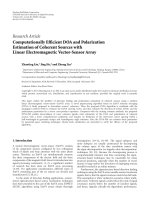
in the “mood space” as shown in Figure 1(a).Thayer[8]
adopted this idea and divided the “mood space” in four
quadrants as depicted in Figure 1(b). This model mainly has
been used in recent research [9–11], probably because it leads
to two binary classification problems with comparably low
complexity.
1.1.2. Audio Features and Metadata. Another task involved
in mood recognition is the selection of features as a base
for the used learning algorithm. This data either can be
directly calculated from the raw audio data or metadata
about the piece of music. The former further divide into
so-called high- and low-level features. Low-level refers to
the characteristics of the audio wave shape like amplitude
and spectrum. From these characteristics more abstract—
or high-level—properties describing concepts like rhythm or
harmonics can be derived. Metadata involves all information
that can be found about a music track. This begins at
essential information like title or artist and ranges from
musical genre to lyrics.
Li and Ogihara [5] extracted a 30-element feature vector
containing timbre, pitch, and rhythm features using Marsyas
[12], a software framework for audio processing with specific
emphasis on Music Information Retrieval applications.
Liu [9] used music in a uniform format (16 kHz, 16 bits,
mono channel) and divided into non-overlapping 32 ms
long frames. Then timbre features based on global spectral
and subband features were extracted. Global spectrum

features were centroid, bandwidth, roll off,andspectral
flux. Subband features were octave-based (7 subbands from
0 to 8 kHz) and consist of the minimum, maximum, and
averageamplitudevalueforeachsubband.Therootmean
square of an audio signal is used as an intensity feature. For
extracting rhythm information only the audio information
of the lowest subband was used. The amplitude envelope
was extracted by use of a hamming window. Edge detection
with a Canny estimator delivered a so-called rhythm curve
in which peaks were detected as bass instrumental onsets.
The average strength of peaks then was used as an estimate
for the strength of the rhythm. Auto-correlation delivered
information about the regularity of the rhythm and the
common divisor of the correlation peaks was interpreted as
the average tempo. Lu et al. [10] continued the work of Liu
using the same preprocessing of audio files. Also the timbre
and intensity features were identical. To calculate the rhythm
curve this time, all subbands were taken into account. The
amplitude envelope was extracted for each subband audio
signal using a half-Hanning window. A Canny edge detector
was used on it to calculate an onset curve. All subband onset
curves were then summed up to deliver the rhythm curve
from which strength, regularity, and tempo were calculated
as explained above.
Trohidis et al. [13] also used timbre and rhythm fea-
tures, which were extracted as described in the following:
two estimates for tempo (bpm) (beats per minute) were
calculated by identifying peaks in an autocorrelated beat
histogram. Additional rhythmic information from the beat
histogram was gathered by calculating amplitude ratios

and summing of histogram ranges. Timbre features were
extracted from the Mel Frequency Cepstral Coefficients
(MFCC) [14] and the Short-Term Fourier Transform (FFT),
which were both calculated per sound frame of 32 ms
duration. From the MFCCs the first 13 coefficients were
taken and from the FFT the spectral characteristics centroid,
roll off, and flux were derived. Additionally, mean and
standard deviation of these features were calculated over all
frames.
Peeters [15] used the following three feature groups in
his submission for the MIREX 2008, (ic-
ir.org/mirex/2008/) audio mood classification task: MFCC,
SFM/SCM, and Chroma/PCP The MFCC features were
13 coefficients including the DC component. SFM/SCM
are the so-called Spectral Flatness and Spectral Crest
Measures. They capture information about whether the
spectrum energy is concentrated in peaks or if it is flat.
Peaks are characteristic for sinusoidal signals while a flat
spectrum indicates noise. Chroma/PCP or Pitch Class Profile
represents the distribution of signal energy among the pitch
classes (refer to Section 2.3).
EURASIP Journal on Audio, Speech, and Music Processing 3
1.1.3. Algorithms and Results. Like with mood taxonomies
there is still no agreed consensus on the learning algorithms
to use for mood prediction. Obviously, the choice highly
depends on the selected mood model. Recent research,
which deals with a four-class dimensional mood model
[9, 10], uses Gaussian Mixture Models (GMM) as a base
for a hierarchical classification system (HCS): at first a
binary decision on arousal is made using only rhythm

and timbre features. The following valence classification is
then derived from the remaining features. This approach
yields an average classification accuracy of 86.3%, based
on a database of 250 classical music excerpts. Additionally,
the mood tracking method presented there is capable of
detecting mood boundaries with a high precision of 85.1%
and a recall of 84.1% on a base of 63 boundaries in 9 pieces
of classical music.
Recently the second challenge in audio mood classifica-
tion was held as a part of the MIREX 2008. The purpose
of this contest is to monitor the current state of research:
this year’s winner in the mood classification task, Peeters
[15], achieved an overall accuracy of 63.7% on the five mood
classes shown in Table 2 before the second placed participant
with 55.0% accuracy.
1.2. This Work. Having presented the current state of re-
search in automatic mood classification the main goals for
this article are presented.
1.2.1. Aims. The first aim of this work is to build up a
music database of annotated music with sufficient size. The
selected music should cover today’s popular music genres.
So this work puts emphasis on popular rather than classical
music. In contrast to most existing work no preselection
of songs is performed, which is presently also considered a
major challenge in the related field of emotion recognition
in human speech [16, 17]. It is also attempted to deal with
ambiguous songs. For that purpose, a mood model capable
of representing ambiguous mood is searched.
Most existing approaches exclusively use low-level fea-
tures. So in this work middle-level features that partly

base on preclassification are additionally used and tested
for suitability to improve the classification. Another task is
the identification of relevant features by means of feature
relevance analysis. This step is important because it can
improve classification accuracy while reducing the number
of attributes at the same time. Also all feature extraction is
based on the whole song length rather than to select excerpts
of several seconds and operate only on them.
The final and main goal of this article is to predict a song’s
mood under real world conditions, that is, by using only
meta information available on-line, no preselection of music,
and compressed music, as reliably as possible. Additionally,
factors limiting the classification success shall be identified
and addressed.
1.2.2. Structure. Section 2 deals with the features that
are used as the informational base for machine learning.
Section 3 contains a description of the music database and all
experiments that are conducted. Finally, Section 4 presents
the experiments’ results, and Section 5 concludes the most
important findings.
2. Features
Like in every machine learning problem it is crucial for
the success of mood detection to select suitable features.
Thosearefeatureswhichconveysufficient information on
the music in order to enable the machine learning algorithm
to find correlations between feature and class values. Those
features either can be extracted directly from the audio data
or retrieved from public databases. Both types of features are
used in this work and their use for estimating musical mood
is investigated. Concerning musical features, both low-level

features like spectrum and middle-level features like chords
are employed.
2.1. Lyrics. In the field of emotion recognition from speech
it is commonly agreed that textual information may help
improve over mere acoustic analysis [18, 19]. For 1937
of 2648 songs in the database (cf. Section 3.1)lyricscan
automatically be collected from two on-line databases: in a
first run lyricsDB, ( is applied,
which delivers lyrics for 1 779 songs, then LyricWiki,
( is searched for all remaining
songs, which delivers lyrics for 158 additional songs.
LyricsDB The only post-processing needed is to remove
obvious “stubs”, that is, lyrics containing only some words
when the real text is much longer. However, this procedure
does not ensure that the remainder of the lyrics is complete
orcorrectatall.Ithastoberemarkedthatnotonlyword
by word transcripts of a song are collected, but that there are
inconsistent conventions used among the databases. So some
lyrics contain passages like “Chorus x2” or “(Repeat)”, which
makes the chorus appear less often in the raw text than it can
be heard in a song. To extract information from the raw text
that is usable for machine learning, two different approaches
are used, as follows.
2.1.1. Semantic D atabase for Mood Estimation. The first
approach is using ConceptNet [20, 21], a text-processing
toolkit that makes use of a large semantic database auto-
matically generated from sentences in the Open Mind Com-
mon Sense Project, ( The
software is capable of estimating the most likely emotional
affect in a raw text input. This has already been shown

quite effective for valence prediction in movie reviews [21].
Listing 1 displays the output for an example song.
The underlying algorithm profits from a subset of
concepts that are manually classified into one of six emo-
tional categories (happy, sad, angry, fearful, disgusted, and
surprised). Now the emotional affect of unclassified concepts
that are extracted from the song’s lyrics can be calculated by
finding and weighting paths which lead to those classified
concepts.
The program output is directly used as attributes. Six
nominal attributes with the emotional category names as
4 EURASIP Journal on Audio, Speech, and Music Processing
(“sad”, 0.579)
(“happy”, 0.246)
(“fearful”, 0.134)
(“angry”, 0.000)
(“disgusted”, 0.000)
(“surprised”, 0.000)
Listing 1: ConceptNet lyrics mood estimation for the song “(I Just)
Died In Your Arms” by Cutting Crew.
possible values indicate which mood is the most, second, ,
least dominant in the lyrics. Six additional numeric attributes
contain the corresponding probabilities. Note that other
alternatives exist, as the word lists found in [22], which
directly assigns arousal and valence values to words, yet
consist of more limited vocabulary.
2.1.2. Text Processing. The second approach uses text pro-
cessing methods introduced in [23] and shown efficient for
sentiment detection in [19, 21]. The raw text is first split
into words while removing all punctuation. In order to

recognise different flexions of the same word (e.g., loved,
loving, loves should be counted as love), the conjugated word
has to be reduced to its word stem. This is done using
the Porter stemming algorithm [24]. It is based on the
following idea: each (English) word can be represented in
the form [C](VC)
m
[V], where C(V)denotesasequence
of one or more consecutive consonants (vowels) and m is
called the measure of the word ((VC)
m
here means an m-
fold repetition of the string VC). Then, in five separated
steps, replacement rules are applied to the word. The first step
deals with the removal of plural and participle endings. The
steps 2 to 5 then replace common word endings like ATION
→ ATE or IVENESS → IVE. Many of those rules contain
conditions under which they may be applied. For example,
the rule “(m>0) TIONAL
→ TION” only is applied when
the remaining stem has a measure greater than zero. This
leaves the word “rational” unmodified while “occupational”
is replaced. If more than one rule matches in a step, the rule
with the biggest matching suffix is applied.
A numerical attribute is generated for each word stem
that is not in the list of stopwords and occurs at least ten times
in one class. The value can be zero if the word stem cannot
be found in a song’s lyrics. Otherwise, if the word occurs, the
number of occurrences is ignored, and the attribute value is
set to one, only normalised to the total length of the song’s

lyrics. This is done to estimate the different prevalence of one
word in a song dependent on the total amount of text.
The mood associated with this numerical representation
of words contained in the lyrics is finally learned by the
classifier as for any acoustic feature. Note that the word
order is neglected in this modelling. One could also consider
compounds of words by N-grams, that is, N consecutive
words. Yet, this usually demands for considerably higher
amounts of training material as the feature space is blown
up exponentially. In our experiments this did not lead to
improvements on the tasks presented in the ongoing.
2.2. Metadata. Additional information about the music is
sparse in this work because of the large size of the music
collection used (refer to Section 3.1): besides the year of
release only the artist and title information is available for
each song. While the date is directly used as a numeric
attribute, the artist and title fields are processed in a similar
way as the lyrics (cf. Section 2.1.2 for a more detailed
explanation of the methods): only the binary information
about the occurrence of a word stem is obtained. The word
stems are generated by string to word vector conversion
applied to the artist and title attributes. Standard word
delimiters are used to split multiple text strings to words
and the Porter stemming algorithm [24]reduceswordsto
common stems in order to map different forms of one word
to their common stem. To limit the number of attributes
that are left after conversion, a minimum word frequency
is set, which determines how often a word stem must occur
within one class. While the artist word list looks very specific
to the collection of artists in the database, the title word list

seems to have more general relevance with words like “love”,
“feel”, or “sweet”. In total, the metadata attributes consist of
one numeric date attribute and 152 binary numeric word
occurrence attributes.
2.3. Chords. A musical chord is defined as a set of three
(sometimes two) or more simultaneously played notes. A
note is characterised by its name—which is also referred to
as pitch class—and the octave it is played in. An octave is
a so-called interval between two notes whose corresponding
frequencies are at a ratio of 2 : 1. The octave is a special
interval as two notes played in it sound nearly equal. This is
why such notes share the same name in music notation. The
octave interval is divided into twelve equally sized intervals
called semitones. In western music these are named as shown
in Figure 2 which visualises these facts. In order to classify
a chord, only the pitch classes (i.e., the note names without
octave number) of the notes involved are important. There
are several different types of chords depending on the size of
intervals between the notes. Each chord type has a distinct
sound which makes it possible to associate it with a set of
moods as depicted in Table 3.
2.3.1. Recognition and Extraction. For chord extraction from
the raw audio data a fully automatic algorithm as presented
by Harte and Sandler [26] is used. Its basic idea is to map
signal energy in frequency subbands to their corresponding
pitch class which leads to a chromagram [27] or pitch
class profile (PCP). Each possible chord type corresponds
to specific pattern of tones. By comparing the chromagram
with predefined chord templates, an estimate of the chord
type can be made. However, also data-driven methods can

be employed [28]. Table 4 shows the chord types that are
recognised. To determine the tuning of a song for a correct
estimation of semitone boundaries, a 36-bin chromagram is
calculated first. After tuning, an exact 12-bin chromagram
can be generated which represents the 12 different semitones.
EURASIP Journal on Audio, Speech, and Music Processing 5
Table 3: Chord types and their associated emotions [25].
Chord Type
Example Associated Emotions
Major
C Happiness, cheerfulness, confidence, satisfaction, brightness
Minor
Cm Sadness, darkness, sullenness, apprehension, melancholy, depression, mystery
Seventh
C
7
Funkiness, moderate edginess, soulfulness
Major Seventh
C
maj7
Romance, softness, jazziness, serenity, exhilaration, tranquillity
Minor Seventh
Cm
7
Mellowness, moodiness, jazziness
Ninth
C
9
Openness, optimism
Diminished

Cdim Fear, shock, spookiness, suspense
Suspended Fourth
C
sus4
Delightful tension
Seventh, Minor Ninth
C
7/9
Creepiness, ominousness, fear, darkness
Added Ninth
C
add9
Steeliness, austerity
Pleasure
Alarmed
Aroused
Afraid
Te n s e
Angry
Distressed
Annoyed
Frustrated
Excited
Astonished
Delighted
Glad
Happy
Pleased
Miserable
Depressed

Sad
Gloomy
Bored
Droopy
Tired
Satisfied
Content
Serene
Calm
At ease
Relaxed
Sleepy
Arousal
•
•
•
•
•
•
•
•
•
•
•
•
•
•
•
•
•

•
•
•
•
•
•
•
•
•
•
•
(a)
Anxious
(tense-energy)
Exuberance
(calm-energy)
Depression
(tense-tiredness)
Contentment
(calm-tiredness)
Te n s e a r o u s a l
Te n s e C a l m
Energetic arousal
Tired
Energy
(b)
Figure 1: Dimensional mood model development: (a) shows a
multidimensional scaling of emotion-related tags suggested by
Russell [7]. (b) is Thayer’s model [8] with four mood clusters.
Height

B
n+1
B
n
A
A#
B
C
C#
D
D#
E
F
F#
G
G#
Chroma
Figure 2: The pitch helix as presented in [26]. The height axis is
associated with a note’s frequency and the rotation corresponds to
the pitch class of a note. Here, B
n
is one octave below B
n+1
.
Table 4: Chord types which are recognised and extracted.
Chord Type Example
Augmented C
+
Diminished Adim
Diminished7 Cdim

7
Dominant7 G
7
Major F

Major7 D
maj7
Minor Gm
Minor7 Cm
7
MinorMajor7 F

m
maj7
The resulting estimate gives the chord type (e.g., major,
minor, diminished) and the chord base tone (e.g., C, F, G
)
(cf. [29] for further details).
6 EURASIP Journal on Audio, Speech, and Music Processing
2.3.2. Postprocessing. Timing information are withdrawn
and only the sequence of recognised chords are used
subsequently. For each chord name and chord type the
number of occurrences is divided by the total number of
chords in a song. This yields 22 numeric attributes, 21
describing the proportion of chords per chord name or type,
and the last one is the number of recognised chords.
2.4. Rhythm Features. Widespread methods for rhythm
detection make use of a cepstral analysis or autocorrelation in
order to perform tempo detection on audio data. However,
cepstral analysis has not proven satisfactory on music

without strong rhythms and suffers from slow performance.
Both methods have the disadvantages of not being applicable
to continuous data and not contributing information to beat
tracking.
The rhythm features used in this article rely on a method
presentedin[30, 31] which itself is based on former work
by Scheirer [32].Itusesabankofcombfilterswithdifferent
resonant frequency covering a range from 60 to 180 bpm.
The output of each filter corresponds to the signal energy
belonging to a certain tempo. This approach has several
advantages: it delivers a robust tempo estimate and performs
well for a wide range of music. Additionally, its output can
be used for beat tracking which strengthens the results by
being able to make easy plausibility checks on the results.
Further processing of the filter output determines the base
meter of a song, that is, how many beats are in each measure
and what note value one beat has. The implementation used
can recognise whether a song has duple (2/4, 4/4) or triple
(3/4, 6/8) meter.
The implementation executes the tempo calculation in
two steps: first, the so called “tatum” tempo is searched.
The tatum tempo is the fastest perceived tempo present in
a song. For its calculation 57 comb filters are applied to the
(preprocessed) audio signal. Their outputs are combined in
the unnormalised tatum vector T

.
(i) The meter vector M
= [m
1

···m
19
]
T
consists of
normalised entries of score values. Each score value
m

i
determines how well the tempo θ
T
· i resonates
with the song.
(ii) The Tatum vector T
= [t
1
···t
57
]
T
is the normalised
vector of filter bank outputs.
(iii) Tatum candidates θ
T1
, θ
T2
are the tempi corre-
sponding to the two most dominant peaks T

.The

candidate with the higher confidence is called the
tatum tempo θ
T
.
(iv) The main tempo θ
B
is calculated from the meter
vector M. Basically, the tempo which resonates best
with the song is chosen.
(v) The tracker tempo θ
BT
is the same as main tempo, but
refined by beat tracking. Ideally, θ
B
and θ
BT
should
be identical or vary only slightly due to rhythm
inaccuracies.
(vi)ThebasemeterM
b
and the final meter M
f
are the
estimates whether the songs has duple or triple meter.
Both can have one of the possible values 3 (for triple)
or4(forduple).
(vii) The tatum maximum T
max
is the maximum value of

T

.
(viii) The tatum mean T
mean
is the mean value of T

.
(ix) The tatum ratio T
ratio
is calculated by dividing the
highest value of T

by the lowest.
(x) The tatum slope T
slope
the first value of T

divided by
the last value.
(xi) The tatum peak distance T
peakdist
is the mean of the
maximum and minimum value of T

normalised by
the global mean.
This finally yields 87 numeric attributes, mainly consist-
ing of the tatum and meter vector elements.
2.5. Spectral Features. First the audio file is converted to

mono, and then a fast Fourier transform (FFT) is applied
[33]. For an audio signal which can be described as x :
[0, T]
→ R, t → x(t), the Fourier transform is defined as
X( f )
=

T
0
x(t)e
−j2πft
dt:
E :
=

∞
0


X

f



2
df ,
(1)
and with the centre of gravity f
c

the nth central moment is
introduced as
M
n
:=
1
E

∞
0

f − f
c

n


X

f



2
df.
(2)
To represent the global characteristics of the spectrum, the
following values are calculated and used as features.
(i) The centre of gravity f
c

.
(ii) The standard deviation which is a measure for how
much the frequencies in a spectrum can deviate from
the centre of gravity. It is equal to

M
2
.
(iii) The skewness which is a measure for how much the
shape of the spectrum below the centre of gravity is
different from the shape above the mean frequency. It
is calculated as M
3
/(M
2
)
1.5
.
(iv) The kurtosis which is a measure for how much the
shape of the spectrum around the centre of gravity
is different from a Gaussian shape. It is equal to
M
4
/

M
2
−3.
(v) Band energies and energy densities for the following
seven octave based frequency intervals: 0 Hz–200 Hz,

200 Hz–400 Hz, 400 Hz–800 Hz, 800Hz–1.6 kHz,
1.6 kHz–3.2 kHz, 3.2 kHz–6.4 kHz, and 6.4 kHz–
12.8 kHz.
3. Experiments
3.1. Database. For building up a ground truth music
database the compilation “Now That’s What I Call Music!”
(U. K. series, volumes 1–69, double CDs, each) is selected.
EURASIP Journal on Audio, Speech, and Music Processing 7
−2 −1012
−2
−1
0
1
2
Va le nce
Arousal
Negative Positive
Passive Active
Figure 3: Dimensional mood model with five discrete values for
arousal and valence.
It contains 2648 titles— roughly a week of continuous total
play time—and covers the time span from 1983 until now.
Likewise it represents very well most music styles which are
popular today; that ranges from Pop and Rock music over
Rap, R&B to electronic dance music as Techno or House. The
stereo sound files are MPEG-1 Audio Layer 3 (MP3) encoded
using a sampling rate of 44.1 kHz and a variable bit rate of
at least 128 kBit/s as found in many typical use-cases of an
automatic mood classification system.
Like outlined in Section 1.1.1, a mood model based

on the two dimensions valence (
=: ν)andarousal(=: α)
is used to annotate the music. Basically, Thayer’s mood
model is used, but with only four possible values (ν, α)
∈
(1, 1), (−1, 1),(−1, −1), (1, −1) it seems not to be capable
to cover the musical mood satisfyingly. Lu backs this
assumption:
“[
·] We find that sometimes the Thayer’s model
cannot cover all the mood types inherent in a
music piece. [
···] We also find that it is still
possible that an actual music clip may contain
some mixed moods or an ambiguous mood.” [10]
A more refined discretisation of the two mood dimen-
sions is needed. First a pseudo-continuous annotation was
considered, that is, (ν, α)
∈ [−1, 1] × [−1, 1], but after the
annotation of 250 songs that approach showed to be too
complex in order to achieve a coherent rating throughout the
whole database. So the final model uses five discrete values
per dimension. With D :
= {−2, −1, 0, 1, 2}all songs receive a
rating (ν, α)
∈ D
2
as visualised in Figure 3.
Songs were annotated as a whole: many implementations
have used excerpts of songs to reduce computational effort

and to investigate only on characteristic song parts. This
either requires an algorithm for automatically finding the
relevant parts as presented, for example, in [34–36]or
[37], or needs selection by hand, which would be a clear
simplification of the problem. Instead of performing any
selection, the songs are used in full length in this article to
stick to real world conditions as closely as possible.
Respecting that mood perception is generally judged
as highly subjective [38], we decided for four labellers. As
stated, mood may well change within a song, as change
of more and less lively passages or change from sad to a
positive resolution. Annotation in such detail is particularly
time-intensive, as it not only requires multiple labelling, but
additional segmentation, at least on the beat-level. We thus
decided in favour of a large database where changes in mood
during a song are tried to be “averaged” in annotation, that
is, assignment of the connotative mood one would have at
first on mind related to a song that one is well familiar
with. In fact, this can be very practical and sufficient in
many application scenarios, as for automatically suggestion
that fits a listener’s mood. A different question though is,
whether a learning model would benefit from a “cleaner”
representation. Yet, we are assuming the addressed music
type—mainstream popular and by that usually commercially
oriented—music to be less affected by such variation as, for
example, found in longer arrangements of classical music.
In fact, a similar strategy is followed in the field of human
emotion recognition: it has been shown that often up to less
than half of the duration of a spoken utterance portrays the
perceived emotion when annotated on isolated word level

[39]. Yet, emotion recognition from speech by and large
ignores this fact by using turn-level labels as predominant
paradigm rather than word-level based such [40].
Details on the chosen raters (three male, one female,
aged between 23 and 34 years; (average: 29 years) and their
professional and private relation to music are provided in
Ta bl e 5. Raters A–C stated that they listen to music several
hours per day and have no distinct preference of any musical
style, while rater D stated to listen to music every second day
on average and prefers Pop music over styles as Hard-Rock
or Rap.
As can be seen, they were picked to form a well-
balanced set spanning from rather “naive” assessors without
instrument knowledge and professional relation to “expert”
assessors including a club disc jockey (D. J.). The latter can
thus be expected to have a good relationship to music mood,
and its perception by the audiences. Further, young raters
prove a good choice, as they were very well familiar with
all the songs of the chosen database. They were asked to
make a forced decision according to the two dimensions
in the mood plane assigning values in
{−2, −1, 0, 1,2} for
arousal and valence, respectively, and as described. They were
further instructed to annotate according to the perceived
mood, that is, the “represented” mood, not to the induced,
that is, “felt” one, which could have resulted in too high
labelling ambiguity: while one may know the represented
mood, it is not mandatory that the intended or equal
mood is felt by the raters. Indeed, depending on perceived
arousal and valence, different behavioural, physiological, and

psychological mechanisms are involved [41].
Listening was chosen via external sound proof head-
phones in isolated and silent laboratory environment. The
songs were presented in MPEG-1 Audio Layer 3 compression
8 EURASIP Journal on Audio, Speech, and Music Processing
Table 5: Overview on the raters (A–D) by age, gender, ethnicity, professional relation to music, instruments played, and ballroom dance
abilities. The last column indicates the cross-correlation (CC) between valence (V) and arousal (A) for each rater’s annotations.
Rater Age Gender Ethnicity Prof. Relation Instruments Dancing CC(V,A)
A 34 years m European club D. J. guitar, drums/percussion Standard/Latin 0.34
B 23 years m European — piano Standard 0.08
C 26 years m European — piano Latin 0.09
D 32 years f Asian — — — 0.43
Table 6: Mean kappa values over the raters (A–D) for four different calculations of ground truth (GT) obtained either by employing rounded
mean or median of the labels per song. Reduction of classes by clustering of the negative or positive labels, that is, division by two.
No. of Classes GT κκ
1
κ
2
Valence
5 mean 0.307 0.453 0.602
5 median 0.411 0.510 0.604
3 mean 0.440 0.461 0.498
3 median 0.519 0.535 0.561
Arousal
5 mean 0.328 0.477 0.634
5 median 0.415 0.518 0.626
3 mean 0.475 0.496 0.533
3 median 0.526 0.545 0.578
in stereo variable bit rate coding and 128 kBit/s minimum as
for the general processing afterwards. Labelling was carried

out individually and independent of the other raters within
a period of maximum 20 consecutive working days. A
continuous session thereby took a maximum time of two
hours. Each song was fully listened to with a maximum
of three times forward skipping by 30 seconds, followed
by a short break, though the raters knew most songs
in the set very well in advance due to their popular-
ity. Playback of songs was allowed, and the judgments
could be reviewed—however, without knowledge of the
other raters’ results. For the annotation a plugin (available
at to the open source audio
player Foobar: ( />that displays the valence arousal plane colour coded as
depicted in Figure 3 for clicking on the appropriate class.
The named skip of 30 seconds forward was obtained via
hot key.
Based on each rater’s labelling, Table 5 also depicts the
correlation of valence and arousal (rightmost coloumn):
though the raters were well familiar with the general concept
of the dimensions, clear differences are indicated already
looking at the variance among these correlations. The
distribution of labels per rater as depicted in Figure 4
further visualizes the clear differences in perception. (The
complete annotation by the four individuals is available at
/>In order to establish a ground truth that considers every
rater’s labelling without exclusion of instances, or songs,
respectively, that do not possess a majority agreement in
label, a new strategy has to be found: in the literature such
instances are usually discarded, which however does not
reflect a real world usage where a judgment is needed on any
musical piece of a database as its prototypcality is not known

in advance or, in rare works subsumed as novel “garbage”
class [17].Thelatterwasfoundunsuitedinourcase,asthe
perception among the raters differs too strongly, and a learnt
model is potentially corrupted too strongly by such a garbage
class that may easily “consume” the majority of instances due
to its lack of sharp definition.
We thus consider two strategies that both benefit from
the fact that our “classes” are ordinal, that is, they are based
on a discretised continuum: mean of each rater’s label or
median, which is known to better take care of outliers. To
match from mean or median back to classes, a binning
is needed, unless we want to introduce novel classes “in
between” (consider the example of two raters judging “0” and
two “1”: by that we obtain a new class “0.5”). We choose a
simple round operation to this aim of preserving the original
five “classes”.
To evaluate which of these two types of ground truth
calculation is to be preferred, Table 6 shows mean kappa
values with none (Cohen’s), linear, and quadratic weighting
over all raters and per dimension. In addition to the five
classes (in the ongoing abbreviated as V5 for valence and
A5 for arousal), it considers a clustering of the positive and
negative values per dimensions, which resembles a division
by two prior to the rounding operation (V3 and A3, resp.).
An increasing kappa coefficient by going from no weight-
ing to linear to quadratic thereby indicates that confusions
between a rater and the established ground truth occur rather
between neighbouring classes, that is, a very negative value is
less often confused with a very positive than with a neutral
one. Generally, kappa values larger 0.4 are considered as good

agreement, while such larger 0.7 are considered as very good
agreement [42].
EURASIP Journal on Audio, Speech, and Music Processing 9
Table 7: Overview on the raters (A–D) by their kappa values for agreement with the median-based inter-labeller agreement as ground truth
for three classes per dimension.
Rater Valence Arousal
κκ
1
κ
2
κκ
1
κ
2
A 0.672 0.696 0.734 0.499 0.533 0.585
B 0.263 0.244 0.210 0.471 0.491 0.524
C 0.581 0.605 0.645 0.512 0.524 0.547
D 0.559 0.596 0.654 0.620 0.633 0.656
43 55 38 19 14
41 179 183 71 28
7 110 333 163 49
11 124 434 288 81
6 24 126 147 74
−2 −10 1 2
−2
−1
0
1
2
Va le nce

Arousal
(a) Rater A
414354411
20 80 145 139 15
28 303 658 324 39
13 110 390 116 14
13287233
−2 −10 1 2
−2
−1
0
1
2
Va le nce
Arousal
(b) Rater B
2171580
37 132 159 101 34
86 446 617 323 30
4 121 303 132 22
1 8 23 24 3
−2 −10 1 2
−2
−1
0
1
2
Va le nce
Arousal
(c) Rater C

12 23 9 7 0
63 176 202 286 17
6 31 157 366 93
15 74 121 641 232
2136150
−2 −10 1 2
−2
−1
0
1
2
Va le nce
Arousal
(d) Rater D
Figure 4: 5 ×5 class distributions of the music database (2648 total instances) for the annotation of each rater (a)–(d).
Obviously, choosing the median is the better choice—
may it be for valence or arousal, five or three classes. Further,
three classes show better agreement unless when considering
quadratic weighting. The latter is however obvious, as less
confusions with far spread classes can occur for three classes.
The choice of ground truth for the rest of this article thus is
either (rounded) median after clustering to three classes, or
each rater’s individual annotation.
In Table 7 the differences among the raters with respect
to accordance to this chosen ground truth strategy—three
10 EURASIP Journal on Audio, Speech, and Music Processing
24 22 6 3 0
45 322 144 76 6
8 139 362 270 23
3 57 298 638 101

0195437
−2 −10 1 2
−2
−1
0
1
2
Va le nce
Arousal
Figure 5: 5 × 5 class distribution of the music database (2648 total
instances) after annotation based on rounded median of all raters.
degrees per dimension and rounded median—are revealed.
In particular rater B notably disagrees with the valence
ground truth established by all raters. Other than that,
generally good agreement is observed.
The preference of three over five classes is further
mostly stemming from the lack of sufficient instances
for the “extreme” classes. This becomes obvious looking
at the resulting distribution of instances in the valence-
arousal plane by the rounded median ground truth for the
original five classes per dimension as provided in Figure 5.
This distribution shows a further interesting effect: though
practically no correlation between valence and arousal was
measured for the raters B and C, and not too strong such
for raters A and D (cf. right most coloumn in Table 5), the
agreement of raters seems to be found mostly in favour of
such a correlation: the diagonal reaching from low valence
and arousal to high valence and arousal is considerably more
present in terms of frequency of musical pieces. This may
either stem from the nature of the chosen compilation of

the CDs, which however well cover the typical chart and
aired music of their time, or that generally music with lower
activation is rather found connotative with negative valence
and vice versa (consider hereon the examples of ballads or
“happy” disco or dance music as examples).
The distributions among the five and three classes (as
mentioned by clustering of negative and positive values,
each) individually per dimension shown in Figure 6 further
illustrates the reason to be found in choosing the three over
the five classes in the ongoing.
3.2. Datasets. First all 2648 songs are used in a dataset
named AllInst. For evaluation of “true” learning success,
training, development, and test partitions are constructed:
we decided for a transparent definition that allows easy
reproducibility and is not optimized in any respect: training
and development are obtained by selecting all songs from
odd years, whereby development is assigned by choosing
every second odd year. By that, test is defined using every
even year. The distributions of instances per partition
are displayed in Figure 7 following the three degrees per
dimension.
Once development was used for optimization of classi-
fiers or feature selection, the training and development sets
are united for training. Note that this partitioning resembles
roughly 50%/50% of overall training/test. Performances
could probably be increased by choosing a smaller test
partition and thus increasing the training material. Yet, we
felt that more than 1000 test instances favour statistically
more meaningfull findings.
To reveal the impact of prototypicality, that is, limiting

to instances or musical pieces with clear agreement by a
majority of raters, we additionally consider the sets Min2/4
for the case of agreement of two out of four raters,
while the other two have to disagree among each other,
resembling unity among two and draw between the others,
and the set Min3/4, where three out of four raters have to
agree. Note that the minimum agreement is based on the
original five degrees per dimension and that we consider
this subset only for the testing instances, as we want to keep
training conditions fixed for better transparency of effects of
prototypization. The according distributions are shown in
Figure 8.
3.3. Feature Subsets. In addition to the data partitions, the
performance is examined in dependence on the subset of
attributes used. Refer to Table 8 for an overview of these
subsets. They are directly derived from the partitioning in the
features section of this work. To better estimate the influence
of lyrics on the classification, a special subset called NoLyr is
introduced, which contains all features except those derived
from lyrics. Note in this respect that for 25% (675) songs
no lyrics are available within the two used on-line databases
which was intentionally left as is to again further realism.
3.4. Training Instance Processing. Training on the unmodified
training set is likely to deliver a highly biased classifier due to
the unbalanced class distribution in all training datasets. To
overcome this problem, three different strategies are usually
employed [16, 21, 43]: the first is downsampling, in which
instances from the overrepresented classes are randomly
removed until each class contains the same number of
instances. This procedure usually withdraws a lot of instances

and with them valuable information, especially in highly
unbalanced situations: it always outputs a training dataset
size equal to the number of classes multiplied with number
of instances in the class with least instances. In highly
unbalanced experiments, this procedure thus leads to a
pathological small training set. The second method used
is upsampling, in which instances from the classes with
proportionally low numbers of instances are duplicated
to reach a more balanced class distribution. This way no
instance is removed from the training set and all information
can contribute to the trained classifier. This is why random
EURASIP Journal on Audio, Speech, and Music Processing 11
Table 8: Feature subsets for attribute dependent analysis of classifier success.
Name Description No. Section
Cho Chord attributes 22 2.3
Con ConceptNet’s mood on lyrics 12 2.1.1
Lyr Word occurrences in lyrics 393 2.1.2
Meta Date, artist and title related 153 2.2
Rhy for rhythmic features 87 2.4
Spec for spectral features 24 2.5
All unision of the above 691 —
NoLyr All without Lyr and Con 286 3.3
−2 −10 1 2
80
541
819
1041
167
(a) Valence V5
−2 −10 1 2

55
593
802
1097
101
(b) Arousal A5
−10 1
621
819
1208
(c) Valence V3
−10 1
648
802
1198
(d) Arousal A3
Figure 6: Class distributions of AllInst in the original V5 and A5 and clustered V3 and A3 versions.
upsampling to forced equal class distribution is chosen
in this article throughout. To not falsify the classification
results, it is important that only the training instances are
upsampled. For upsampling a target size of 200% (number
of instances) of the upsampled training dataset compared
to the original dataset is employed. Likewise replacement of
instances is allowed so that equal class distribution is also
achievable in highly unbalanced experiments. At the same
time it is ensured that each original instance is preserved in
the training material. Apart from the fact that a mixed up-,
and down-sampling strategy can be followed as compromise
between the above, a third variant is assignment of different
weighting of instances for the computation of the classifier

objectivefunction.Inpractice,thisisoftenactuallyoften
solved by classifier internal upsampling, and may lead to
less stable results, while not providing any advantage in our
respect, as obtainable performances are not higher, which is
why this variant was not further pursued. However, this may
be well of interest in an on-line system which needs to be
adapted, for example, when a user labels a new song to adapt
his audio-playing device.
Finally, the classifier success highly depends on a reliable
feature selection. As there are 691 attributes in total, it is
crucial to identify redundant or useless attributes and remove
them before applying the classifier on the training data.
We approach this topic in two ways: first we are interested
to find the most relevant attributes. For that we decide
for a vertical view and divide by group measuring the
“value” by a classification task. Second, we want to see
obtainable boost deriving from a better representation of
the problem in a more compact feature space that is freed
of irrelevant correlated information. This is best obtained
by employing the target classifier in a “wrapper” manner
and its accuracy as evaluation measure. Given the size of
the data set and the feature space, a search function is
mandatory, as exhaustive search becomes computationally
prohibitive. A simple, yet highly efficient method to this
aim is “conservative hill climbing”, that is, deciding for the
best feature at the time starting from none and adding the
“next best”, each. As this obviously is prone to nesting effects,
one usually adds a back stepping option whether “another
previous candidate” would have better suited. This is known
12 EURASIP Journal on Audio, Speech, and Music Processing

413 150 85
147 362 293
61 307 830
−10 1
−1
0
1
Va le nce
Arousal
(a) All
103 42 27
37 97 86
20 72 206
−10 1
−1
0
1
Va le nce
Arousal
(b) Train
112 35 25
39 91 81
15 68 220
−10 1
−1
0
1
Va le nce
Arousal
(c) Development

198 73 33
71 174 126
26 167 404
−10 1
−1
0
1
Va le nce
Arousal
(d) Test
Figure 7: 3 × 3 class distribution of the music database (2648 total instances) after annotation based on rounded median of all raters and
clustering of positive and negative instances. Shown are all, train, development, and test instances.
Allinst min 2/4 min 3/4
1272
1042
516
(a) Valence
Allinst min 2/4 min 3/4
1272
974
509
(b) Arousal
Figure 8: Distributions of test instances in dependence of prototypicality: AllInst, Min2/4 (minimum 2 of 4 raters agree), and Min3/4
(minimum 3 of 4 raters agree).
as floating, and with the described forward addition as
Sequential Forward Floating Search. As a result, one obtains
a horizontal view, which is usually hard to interpret: features
in the optimal set, which is found by best performance on
the development set, are usually a mixture of all groups.
Yet, it is not clear whether these are the best due to the

suboptimal nature inherent in any search function and
the fact that it de-correlates the space rather than ranks.
By that the value of a feature is unclear, as is whether
a picked feature does not have a counter-part of similar
characteristics that was not picked, as only one of a sort is
needed.
EURASIP Journal on Audio, Speech, and Music Processing 13
Table 9: Lassification accuracies (acc), mean precision (pre), and mean recall (rec) for classification on AllInst test data against different
attribute subsets for the V3 and A3 tasks, SVM.
Type Valence Arousal
% acc pre rec acc pre rec
All 51.3 49.9 50.9 50.0 49.5 50.5
Cho 47.6 47.4 49.2 47.0 48.2 50.0
Con 38.4 35.8 35.9 28.9 32.8 33.5
Lyr 40.5 36.8 37.8 36.8 38.8 39.4
Meta 35.5 39.1 39.3 36.1 38.3 37.4
NoLyr 58.5 57.6 58.8 53.3 52.6 54.1
Rhy 56.4 56.3 57.7 52.4 51.7 54.0
Spec 47.5 48.1 48.8 47.6 47.0 49.0
Table 10: Overview on the raters (A–D) by accuracy (acc), precision (pre), and recall (rec) for the V3 and A3 tasks based on each rater’s
individual labels. Feature set NoLyr, set AllInst, SVM.
Rater Valence Arousal
% acc pre rec acc pre rec
A 57.6 57.1 58.5 43.6 42.7 43.4
B 48.1 47.3 48.5 60.0 59.1 63.8
C 53.5 53.3 55.3 52.0 49.5 53.0
D 56.3 48.9 54.2 46.9 46.7 47.8
3.5. Classifier. The classifier used in the first order is Support
Vector Machines (SVM) trained with Sequential Minimal
Optimisation (SMO) [44], the complexity value c set to 1.0

and a linear kernel function. Multiclass discrimination is
reached by a pairwise 1-versus-1 strategy. The best choice of
c is determined by calculating the classifier accuracy of two
classification tasks (V3 and A3) for c
∈{0.5, 1.0,1.5, 2.0, 2.5}
on the development set. Increasing the exponent value of
the Kernel function was considered, but showed to have no
positive effect on the classifier accuracy.
In addition, further classifiers will be used in one
experiment for exploration on classifier choice.
4. Results
All results are provided by accuracy, that is, the number of
correctly assigned instances divided by the total number of
instances. In addition, we provide the mean precision and
recall, which are obtained without weighting by number
of instances per class (note that weighting the recall prior
to mean calculation resembles the accuracy). By that the
imbalance of songs among classes is better reflected, and one
has a good feeling of chance level: for mean recall this simply
depends on the number of classes, which in our case are three
throughout, as we consider valence and arousal separately.
4.1. Effects of Feature Group. As first experiment we want to
measure the relevance of each feature group as introduced
in Section 3.3 To this aim we consider the ground truth by
rounded median and all instances and classify per group in
isolation. In Table 9, these results are summarised, whereas
Figures 9 and 10 depict according confusions matrices per
type.
The recognition rates clearly illustrate the challenge of
the task: some groups as the concepts or even lyrics are

found hardly above chance level when used on their own.
Surprisingly low differences are further observed between
performances per type among valence and arousal. The fact
that all features in union are inferior to the set without
lyrics clearly shows the too high dimensionality of the
feature space. Most notably, the rhythm features which
in this form are introduced in this work for the task of
mood detection, are almost on par to the complete set
without lyrics and by that also significantly outperform
spectral features. The latter are also outperformed by
the chord-based features, which overall emphasizes the
high suitability of the middle-level rhythmic and chord
features.
The confusion matrices for the NoLyr and Rhy sets
show fewer confusions among the classes further spread
apart which adds to the practicability of the results: negative
or positive is more likely confused with neutral than the
opposite.
4.2. Effects of Rater. We next investigate differences between
the different raters in terms of obtainable classification
performance. The according results of the classification tasks,
which consider each rater individually, are presented in
Ta bl e 10 for the NoLyr set, which was found superior in the
previous evaluation and will thus be used in the ongoing. The
tasks are again V3 and A3 on the set AllInst.
Significant differences are found among the raters. Con-
sidering valence, annotation by the professional D. J. leads to
the highest accuracy values. In case of arousal the differences
are even more distinct which may be an indication that
arousal annotation differs even more strongly.

14 EURASIP Journal on Audio, Speech, and Music Processing
68 163 332
106 156 152
165 69 61
−10 1
1
0
−1
Classified as
Real class
(a) All
139 157 267
133 153 128
186 62 47
−10 1
1
0
−1
Classified as
Real class
(b) Cho
124 107 332
122 79 213
104 70 121
−10 1
1
0
−1
Classified as
Real class

(c) Lyr
60 152 351
97 197 120
196 67 32
−10 1
1
0
−1
Classified as
Real class
(d) Nolyr
124 110 329
147 172 95
216 56 23
−10 1
1
0
−1
Classified as
Real class
(e) Rhy
56 237 270
94 153 167
181 73 41
−10 1
1
0
−1
Classified as
Real class

(f) Spec
Figure 9: Valence: confusion matrices for the V3 classification task and selected feature subsets. Classifier SVM, dataset AllInst.
EURASIP Journal on Audio, Speech, and Music Processing 15
108 191 298
83 162 126
176 82 46
−10 1
1
0
−1
Classified as
Real class
(a) All
158 214 225
105 174 92
199 67 38
−10 1
1
0
−1
Classified as
Real class
(b) Cho
148 306 143
92 215 64
110 125 69
−10 1
1
0
−1

Classified as
Real class
(c) Lyr
92 188 317
88 162 121
199 61 44
−10 1
1
0
−1
Classified as
Real class
(d) Nolyr
151 142 304
110 139 122
224 58 22
−10 1
1
0
−1
Classified as
Real class
(e) Rhy
125 201 271
101 142 128
192 54 58
−10 1
1
0
−1

Classified as
Real class
(f) Spec
Figure 10: Arousal: confusion matrices for the A3 classification task and selected feature subsets. Classifier SVM, dataset AllInst.
16 EURASIP Journal on Audio, Speech, and Music Processing
Table 11: Prototypicality effect: classification accuracies (acc), mean precision (pre), and mean recall (rec) for training with the training and
development instances of AllInst, and testing on those of AllInst, Min2/4, and Min3/4. NoLyr feature set, V3 and A3 tasks, selection by SFFS
(of the 286 original features 131 are found as optimal for the A3, and 132 for the V3 task).
Type Valence Arousal
% acc pre rec acc pre rec
AllInst 58.5 57.6 58.8 53.3 52.6 54.1
Min2/4 60.1 59.4 61.1 54.8 54.4 56.7
Min3/4 61.4 61.2 65.5 60.9 61.7 64.9
with feature selection
AllInst 61.0 60.0 61.2 55.2 54.5 56.2
Min2/4 63.0 62.5 64.1 57.2 56.8 59.6
Min3/4 64.1 64.5 68.6 60.9 61.1 64.8
Table 12: Comparison of classifiers: classification accuracies (acc), mean precision (pre), and mean recall (rec) for classification on AllInst
test data with the NoLyr feature set for the V3 and A3 tasks. Considered alternatives to SVM are Random Forests (RF, with 250 trees found
optimal and minor differences in the range between 100–250), a K2 hill climbing structure-learnt Bayesian Network (BN), and k Nearest
Neighbours with Euclidean distance (kNN, with k being 5 found optimal). Feature set NoLyr.
Type Valence Arousal
% acc pre rec acc pre rec
SVM 58.5 57.6 58.8 53.3 52.6 54.1
RF 61.0 60.4 58.3 58.7 56.5 56.2
BN 51.6 51.0 53.1 52.9 51.3 54.0
kNN 45.4 46.8 47.0 44.9 45.3 46.0
4.3. Effects of Prototypicality. To obtain a better impression
in comparison with the predominant studies that limit to
instances that are agreed upon by the majority of raters in

terms of portrayed mood, Table 11 investigates the limitation
of the test instances to those agreed upon by a minimum of
two or three out of four raters as described: the training set
is kept constant based on all instances, while the test set is
accordingly reduced. As to be expected, accuracy is higher
for the instances with higher agreement. These differences
are even stronger for arousal.
In this table we also provide results obtained by feature
selection—this time aiming at increased accuracy rather than
interpretation. By that a gain is reached in accuracy for all
constellations but prototypical arousal. Overall, roughly 8%
are gained absolute by going from all to more prototypical
instances.
4.4. Effects of Classifier. So far we sticked to SVM as classifier
of choice. Naturally, different performances may be obtained
with other such. Table 12 depicts results for a selection that
aims at a good coverage of representatives from different her-
itage while limiting their choice: Random Forests are chosen
as good example of boosted decision trees which at the same
time subsample the feature space and thus inject random
in the bootstrapping and feature optimization process. In
addition they inherit feature selection by their alignment
of decision nodes based on Gain Ratio in combination
with pruning of lower nodes. A structure learned Bayesian
Network was further chosen as representative for statistical
learners. Finally, at the lower end, a simple distance-based k
Nearest Neighbour classifier is chosen.
Parameters have been optimized for the classifiers on the
development set, each, and significant differences are found
between SVM and Random Forests on the “stronger end”

and their counterparts. In this comparison Random Forests
are actually observed superior to SVM. This effect however
was not found to be persistent by repetition of the previously
shown results. They were thus not preferred over SVM, as
less transparency exists in terms of bootstrapping and feature
space subsampling.
Deriving from the ordinal nature of the classes, one can
additionally consider regression approaches (cf. [21, 43]).
Yet, this suffers from the uneven and distinct distribution
as considerably more than four labellers would be needed to
obtain a genuine continuum from the mean values of valence
and arousal.
5. Conclusion
In this paper, a system for automatic music mood prediction
based on musical features and lyrics is presented and tested
against a large database of popular music. A mood model
with three to five class values for the two dimensions valence
and arousal is applied in order to generate a ground truth for
scalable mood prediction with respect to the level of mood
resolution. Due to the mood model design, not only clearly
neutral songs receive a class value of zero, but also those
where some parts are positive and others negative in respect
to the mood dimensions. Less abstractly spoken, a song with
both happy and sad sections can “average” to neutral valence
which makes the song receive a valence value of 0, which
is obviously not the same as a song with no remarkable
EURASIP Journal on Audio, Speech, and Music Processing 17
positive or negative valence. That is why a separate class for
ambiguous songs particularly in this respect (as opposed to
ambiguous due to mismatch in labelling) probably could

improve classification results. Another approach to better
handle ambiguous songs would be to adapt a mood tracking
system as presented by Lu et al. [10] for classical music. This
way music is split into small chunks of constant mood, which
are presumably easier to classify correctly. In this case, an
interesting problem will be to find a clear representation for
the complex prediction made by such a system. Moreover, to
establish a ground truth database for such a system implies—
as stated—considerable efforts. However, automatic music
structure analysis may be considered as tool (e.g., [34, 37]).
The following findings are made concerning the per-
formance of feature groups for different classification tasks:
rhythmic, chord-based, and spectral features are primarily
suitable to determine a song’s valence and arousal. Especially
the rhythm and chord features presented in this work seem
to have high potential. Lyrics surprisingly do not contribute
much to the classification results in these investigations.
Applying the same methods to the artist and title tag is not
considered of higher benefit, either. This may be overcome by
integration of further meta information as usage information
[45]. More research is needed to compare different ways
of generating meaningful features from both metadata and
lyrics. ConceptNet’s mood guess on the lyrics content seems
promising but it does not contribute to the classification
success when applied like presented here.
Dealing with “every music that comes in”, we had
proposed usage of the (rounded) median to provide a label
even in the case of complete rater disagreement. This better
fits the paradigm of a dimensional approach, as introduction
of a garbage class would disrupt the ordinal structure.

Alternatively, we had reduced the test instances by those that
lack such agreement. As to be expected, more prototypical
instances lead to higher performances. By that the overall
accuracies and mean recall rate were found around 60%
in the case of processing all instances, and around 70% in
the case of prototypical representatives for the two three-
class tasks of valence and arousal determination. For these
constellations confusions were observed with the neighbour-
ing classes, which raises practicability. Yet, clearly future
efforts will be needed before systems can fully automatically
judge on musical mood no matter what music is provided.
In addition, high variances between the labellings by four
raters were observed that also led to significantly differing
performances when the system was trained per rater. This
shows that mood perception is indeed rather subjective, and
that it will be challenging at different levels to follow every
user’s perception once a user would be willing to train or
personalize such a system.
Such future work may consider more elaborate low-level
feature extraction, for example, by use of wavelets [46].
Also, estimation of middle-level features as chords can be
improved, for example, by enhancement through musical
source separation [47]. In addition, alternative fusion strate-
gies of features may be followed, for example, by classifying
and optimizing for each feature group individually and
fusing in a late manner opposed to the herein chosen strategy
of accumulating all features in one classifier. While we had
shown the fusion of acoustic and textual information in
this work, future research may further consider integration
of video information such as low-level colour histograms

or even high-level interpretation for the classification of
mood in music videos as shown beneficial in the field of
emotion recognition [43]. The general distinction between
high and low valence and arousal certainly satisfies many
use-cases as mood matching, yet further dimensions may
also be evaluated, as the “dominance” often met in emotion
modelling or self-learnt spaces as introduced in [48]. Finally,
clearly added rater tracks will be of interest and effects on
ground truth stability.
Considering the demonstrated performance in combina-
tion with the proposed and further future work, automatic
music mood detection seems feasible in the near future also
at large scale—though certainly with limited mood model
complexity.
References
[1] M. Tolos, R. Tato, and T. Kemp, “Mood-based navigation
through large collections of musical data,” in Proceedings
of the 2nd IEEE Consumer Communications and Networking
Conference (CCNC ’05), pp. 71–75, Las Vegas, Nev, USA, 2005.
[2] Y. Feng, Y. Zhuang, and Y. Pan, “Popular music retrieval by
detecting mood,” in Proceedings of the 26th International ACM
SIGIR Conference on Research and Development in Information
Retrieval, pp. 375–376, Toronto, Canada, 2003.
[3] K. Hevner, “Experimental studies of the elements of expres-
sion in music,” American Journal of Psychology, vol. 48, pp.
246–268, 1936.
[4] P. R. Farnsworth, The Social Psychology of Music,TheDryden
Press, New York, NY, USA, 1958.
[5] T. Li and M. Ogihara, “Detecting emotion in music,” in Pro-
ceedings of the International Symposium on Music Information

Retrieval (ISMIR ’03), pp. 239–240, 2003.
[6] J. A. Russell, “Measures of emotion,” in The Measurement of
Emotions, vol. 4 of Emotion, Theory, Research, and Experience,
pp. 83–111, Academic Press, San Diego, Calif, USA, 1989.
[7]J.A.Russell,“Acircumplexmodelofaffect,” Journal of
Personality and Social Psychology, vol. 39, no. 6, pp. 1161–1178,
1980.
[8] R.E.Thayer,The Biopsychology of Mood and Arousal,Oxford
University Press, Boston, Mass, USA, 1990.
[9] D. Liu, “Automatic mood detection from acoustic music
data,” in Proceedings of the International Symposium on Music
Information Retrieval (ISMIR ’03), pp. 13–17, 2003.
[10] L. Lu, D. Liu, and H J. Zhang, “Automatic mood detection
and tracking of music audio signals,” IEEE Transactions on
Audio, Speech & Language Processing, vol. 14, no. 1, pp. 5–18,
2006.
[11] Z. Xiao, E. Dellandr
´
ea, W. Dou, and L. Chen, “What is the best
segment duration for music mood analysis?” in Proceedings
of the International Workshop on Content-Based Multimedia
Indexing (CBMI ’08), pp. 17–24, June 2008.
[12] G. Tzanetakis and P. Cook, “Marsyas: a framework for
audio analysis,” Organised Sound, vol. 4, no. 3, pp. 169–175,
December 2000.
[13] K. Trohidis, G. Tsoumakas, G. Kalliris, and I. Vlahavas, “Multi-
label classification of music into emotions,” in Proceedings of
the International Symposium on Music Information Retrieval
(ISMIR ’08), pp. 325–330, 2008.
18 EURASIP Journal on Audio, Speech, and Music Processing

[14] B. Logan, “Mel frequency cepstral coefficients for music
modeling,” in Proceedings of the International Symposium on
Music Information Retrieval (ISMIR ’00), 2000.
[15] G. Peeters, “A generic training and classification system for
MIREX08 classification tasks: audio music mood, audio genre,
audio artist and audio tag,” in Proceedings of the International
Symposium on Music Information Retrieval (ISMIR ’08), 2008.
[16] B. Schuller, S. Steidl, and A. Batliner, “The INTERSPEECH
2009 emotion challenge,” in Proceedings of the 10th Annual
Conference of the International Speech Communication Asso-
ciation (INTERSPEECH ’09), pp. 312–315, Brighton, UK,
September 2009.
[17] S. Steidl, B. Schuller, D. Seppi, and A. Batliner, “The hinterland
of emotions: facing the open-microphone challenge,” in
Proceedings of the 4th International HUMAINE Association
Conference on A ffective Computing and Intelligent Interaction
2009 (ACII ’09), vol. 1, pp. 690–697, IEEE, Amsterdam, The
Netherlands, 2009.
[18] Z J. Chuang and C H. Wu, “Emotion recognition using
acoustic features and textual content,” in Proceedings of
the IEEE Internat ional Conference on Multimedia and Expo
(ICME ’04), vol. 1, pp. 53–56, Taipei, Taiwan, 2004.
[19] B. Schuller, A. Batliner, S. Steidl, and D. Seppi, “Emotion
recognition from speech: putting ASR in the loop,” in
Proceedings of the IEEE International Conference on Acoustics,
Speech and Signal Processing (ICASSP ’09), pp. 4585–4588,
Taipei, Taiwan, 2009.
[20] H. Liu and P. Singh, “ConceptNet—a practical commonsense
reasoning tool-kit,” BT Technology Journal,vol.22,no.4,pp.
211–226, 2004.

[21] B. Schuller, J. Schenk, and G. Rigoll, ““the godfather” vs.
“chaos”: comparing linguistic analysis based on online knowl-
edge sources and bags-of-n-grams for movie review valence
estimation,” in Proceedings of the International Conference on
Document Analysis and Recognition (ICDAR ’09), Barcelona,
Spain, 2009.
[22] M. M. Bradley and P. J. Lang, “Affective norms for english
words (anew): stimuli, instruction manual, and affective
ratings,” Technical Report C–1, Center for Research in Psy-
chophysiology, University of Florida, Gainesville, Fla, USA,
1999.
[23] T. Joachims, “Text categorization with support vector
machines: learning with many relevant features,” in Proceed-
ings of the 10th European Conference on Machine Learning
(ECML ’98), pp. 137–142, Springer, Chemnitz, Germany,
1998.
[24] M. F. Porter, “An algorithm for suffix stripping,” Program, vol.
3, no. 14, pp. 130–137, 1980.
[25] W. Chase, How Music REALLY Works!, Roedy Black, Vancou-
ver, Canada, 2nd edition, 2006.
[26] C. A. Harte and M. Sandler, “Automatic chord identification
using a quantised chromagram,” in Proceedings of the 118th
Convention of the AES, May 2005.
[27] M. M
¨
uller, Information Retrieval for Music and Motion,
Springer, Berlin, Germany, 2007.
[28] K. Lee and M. Slaney, “Acoustic chord transcription and key
extraction from audio using key-dependent HMMs trained
on synthesized audio,” IEEE Transactions on Audio, Speech and

Language Processing, vol. 16, no. 2, pp. 291–301, 2008.
[29] B. Schuller, B. H
¨
ornler, D. Arsic, and G. Rigoll, “Audio chord
labeling by musiological modeling and beat-synchronization,”
in Proceedings of the IEEE International Conference on Multi-
media and Expo (ICME ’09), pp. 526–529, New York, NY, USA,
2009.
[30]B.Schuller,F.Eyben,andG.Rigoll,“Fastandrobustmeter
and tempo recognition for the automatic discrimination of
ballroom dance styles,” in Proceedings of the IEEE Interna-
tional Conference on Acoustics, Speech and Signal Processing
(ICASSP ’07), vol. 1, pp. I217–I220, Honolulu, Hawaii, USA,
2007.
[31] B. Schuller, F. Eyben, and G. Rigoll, “Tango or Waltz?: putting
ballroom dance style into tempo detection,” EURASIP Journal
on Audio, Speech, and Music Processing, vol. 2008, Article ID
846135, 12 pages, 2008.
[32] E. D. Scheirer, “Tempo and beat analysis of acoustic musical
signals,” Journal of the Acoustical Society of America, vol. 103,
no. 1, pp. 588–601, 1998.
[33] P. Boersma, “Praat, a system for doing phonetics by computer,”
Glot International, vol. 5, pp. 341–345, 2001.
[34] M. A. Bartsch and G. H. Wakefield, “To catch a chorus:
using chroma-based representations for audio thumbnailing,”
in Proceedings of the IEEE Workshop on Applications of Signal
Processing to Audio and Acoustics (WASPAA ’01),NewPaltz,
NY, USA, October 2001.
[35] M. Goto, “A chorus section detection method for musical
audio signals and its application to a music listening station,”

IEEE Transactions on Audio, Speech and Language Processing,
vol. 14, no. 5, pp. 1783–1794, 2006.
[36] M. M
¨
uller and F. Kurth, “Towards structural analysis of audio
recordings in the presence of musical variations,” EURASIP
Journal on Advances in Signal Processing, vol. 2007, Article ID
89686, 18 pages, 2007.
[37] B. Schuller, F. Dibiasi, F. Eyben, and G. Rigoll, “One day in
half an hour: music thumbnailing incorporating harmony-
and rhythm structure,” in Proceedings of the 6th Workshop on
Adaptive Multimedia Retrieval (AMR ’08), Berlin, Germany,
2008.
[38]X.Hu,J.S.Downie,C.Laurier,M.Bay,andA.F.Ehmann,
“The 2007 mirex audio mood classification task: lessons
learned,” in Proceedings of the International Symposium on
Music Information Retrieval (ISMIR ’08), pp. 462–467, 2008.
[39] S. Steidl, A. Batliner, D. Seppi, and B. Schuller, “On the impact
of children’s emotional speech on acoustic and language
models,” EURASIP Journal on Audio, Speech, and Music
Processing, vol. 2010, Article ID 783954, 14 pages, 2010.
[40] Z. Zeng, M. Pantic, G. I. Roisman, and T. S. Huang, “A
survey of affect recognition methods: audio, visual, and spon-
taneous expressions,” IEEE Transactions on Pattern Analysis
and Machine Intelligence, vol. 31, no. 1, pp. 39–58, 2009.
[41] A. Gabrielsson, “Emotion perceived and emotion felt: same or
different?” Musicae Scientiae, pp. 123–147, 2002.
[42] J. Carletta, “Squibs and discussions: assessing agreement
on classification tasks: the kappa statistic,” Computational
Linguistics, vol. 22, no. 2, pp. 249–254, 1996.

[43] B. Schuller, R. M
¨
uller, F. Eyben, et al., “Being bored? Recog-
nising natural interest by extensive audiovisual integration for
real-life application,” Image and Vision Computing Journal, vol.
27, no. 12, pp. 1760–1774, 2009.
[44] I. H. Witten and E. Frank, Data Mining: Practical Machine
Learning To ols and Techniques, Morgan Kaufmann, 2nd edi-
tion, 2005.
[45] X. Hu and J. S. Downie, “Exploring mood metadata: relation-
ships with genre, artist and usage metadata,” in Proceedings
of the 8th International Symposium on Music Information
Retrieval (ISMIR ’07), Vienna, Austria, 2007.
[46] F. Kurth and M. Clausen, “Filter bank tree and M-band
wavelet packet algorithms in audio signal processing,” IEEE
Transactions on Signal Processing, vol. 47, no. 2, pp. 549–554,
1999.
EURASIP Journal on Audio, Speech, and Music Processing 19
[47] P. Smaragdis and J. C. Brown, “Non-negative matrix factoriza-
tion for polyphonic music transcription,” in Proceedings of the
International Workshop on Applications of Signal Processing to
Audio and Acoustics (WASPAA ’03), pp. 177–180, IEEE, 2003.
[48] M. W
¨
ollmer, F. Eyben, S. Reiter, et al., “Abandoning emo-
tion classes—towards continuous emotion recognition with
modelling of long-range dependencies,” in Proceedings of the
Annual Conference of the International Speech Communication
Association (INTERSPEECH ’08), pp. 597–600, ISCA, Bris-
bane, Australia, 2008.