báo cáo hóa học:" Research Article Clusters versus GPUs for Parallel Target and Anomaly Detection in Hyperspectral Images" potx

Hindawi Publishing Corporation
EURASIP Journal on Advances in Signal Processing
Volume 2010, Article ID 915639, 18 pages
doi:10.1155/2010/915639
Research Article
Clusters versus GPUs for Parallel Target and
Anomaly Detection in Hyperspectral Images
Abel Paz and Antonio Plaza
Department of Technology of Computers and Communications, University of Extremadura, 10071 Caceres, Spain
Correspondence should be addressed to Antonio Plaza,
Received 2 December 2009; Revised 18 February 2010; Accepted 19 February 2010
Academic Editor: Yingzi Du
Copyright © 2010 A. Paz and A. Plaza. This is an open access article distributed under the Creative Commons Attribution License,
which permits unrestricted use, distribution, and reproduction in any medium, provided the original work is properly cited.
Remotely sensed hyperspectral sensors provide image data containing rich information in both the spatial and the spectral domain,
and this information can be used to address detection tasks in many applications. In many surveillance applications, the size of the
objects (targets) searched for constitutes a very small fraction of the total search area and the spectral signatures associated to the
targets are generally different from those of the background, hence the targets can be seen as anomalies. In hyperspectral imaging,
many algorithms have been proposed for automatic target and anomaly detection. Given the dimensionality of hyperspectral
scenes, these techniques can be time-consuming and difficult to apply in applications requiring real-time performance. In this
paper, we develop several new parallel implementations of automatic target and anomaly detection algorithms. The proposed
parallel algorithms are quantitatively evaluated using hyperspectral data collected by the NASA’s Airborne Visible Infra-Red
Imaging Spectrometer (AVIRIS) system over theWorld Trade Center (WTC) in New York, five days after the terrorist attacks
that collapsed the two main towers in theWTC complex.
1. Introduction
Hyperspectral imaging [1] is concerned with the measure-
ment, analysis, and interpretation of spectra acquired from
a given scene (or specific object) at a short, medium,
or long distance by an airborne or satellite sensor [2].
Hyperspectral imaging instruments such as the NASA Jet
Propulsion Laboratory’s Airborne Visible Infrared Imaging

Spectrometer (AVIRIS) [3] are now able to record the visible
and near-infrared spectrum (wavelength region from 0.4
to 2.5 micrometers) of the reflected light of an area 2 to
12 kilometers wide and several kilometers long using 224
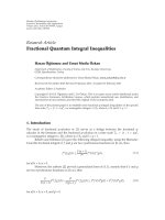
spectral bands. The resulting “image cube” (see Figure 1)
is a stack of images in which each pixel (vector) has an
associated spectral signature or fingerprint that uniquely
characterizes the underlying objects [4]. The resulting data
volume typically comprises several GBs per flight [5].
The special properties of hyperspectral data have signif-
icantly expanded the domain of many analysis techniques,
including (supervised and unsupervised) classification, spec-
tral unmixing, compression, target, and anomaly detection
[6–10]. Specifically, the automatic detection of targets and
anomalies is highly relevant in many application domains,
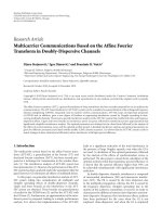
including those addressed in Figure 2 [11–13]. For instance,
automatic target and anomaly detection are considered
very important tasks for hyperspectral data exploitation
in defense and security applications [14, 15]. During the
last few years, several algorithms have been developed
for the aforementioned purposes, including the automatic
target detection and classification (ATDCA) algorithm [12],
an unsupervised fully constrained least squares (UFCLSs)
algorithm [16], an iterative error analysis (IEA) algorithm
[17], or the well-known RX algorithm developed by Reed
and Yu for anomaly detection [18]. The ATDCA algorithm
finds a set of spectrally distinct target pixels vectors using the
concept of orthogonal subspace projection (OSP) [19] in the
spectral domain. On the other hand, the UFCLS algorithm
generates a set of distinct targets using the concept of least

square-based error minimization. The IEA uses a similar
approach, but with a different initialization condition. The
RX algorithm is based on the application of a so-called RXD
filter, given by the well-known Mahalanobis distance. Many
2 EURASIP Journal on Advances in Signal Processing
Atmosphere
Soil
Water
Ve g e t a ti o n
(a)
4 8 12 16 20 24
×10
2
Wavelength (nm)
0
0.2
0.4
0.6
0.8
1
Reflectance
4
812162024
×10
2
Wavelength (nm)
0
0.2
0.4
0.6

0.8
1
Reflectance
4 8 12 16 20 24
×10
2
Wavelength (nm)
0
0.2
0.4
0.6
0.8
1
Reflectance
4 8 12 16 20 24
×10
2
Wavelength (nm)
0
0.2
0.4
0.6
0.8
1
Reflectance
(b)
Figure 1: Concept of hyperspectral imaging.
Military target detection
Mine detection
Crop stress location

Rare mineral detection
Infected trees location
Search-and-rescue
operations
Applications
Geology
Precision agriculture
Forestry
Defense & intelligence Public safety
Figure 2: Applications of target and anomaly detection.
EURASIP Journal on Advances in Signal Processing 3
other target/anomaly detection algorithms have also been
proposed in the recent literature, using different concepts
such as background modeling and characterization [13, 20].
Depending on the complexity and dimensionality of
the input scene [21], the aforementioned algorithms may
be computationally very expensive, a fact that limits the
possibility of utilizing those algorithms in time-critical
applications [5]. In turn, the wealth of spectral information
available in hyperspectral imaging data opens ground-
breaking perspectives in many applications, including target
detection for military and defense/security deployment [22].
In particular, algorithms for detecting (moving or static)
targets or targets that could expand their size (such as
propagating fires) often require timely responses for swift
decisions that depend upon high computing performance of
algorithm analysis [23]. Therefore, in many applications it
is of critical importance that automatic target and anomaly
detection algorithms complete their analysis tasks quickly
enough for practical use. Despite the growing interest in

parallel hyperspectral imaging research [24–26], only a few
parallel implementations of automatic target and anomaly
detection algorithms for hyperspectral data exist in the
open literature [14]. However, with the recent explosion in
the amount and dimensionality of hyperspectral imagery,
parallel processing is expected to become a requirement in
most remote sensing missions [5], including those related
with the detection of anomalous and/or concealed targets.
Of particular importance is the design of parallel algorithms
able to detect target and anomalies at subpixel levels [22],
thus overcoming the limitations imposed by the spatial
resolution of the imaging instrument.
In the past, Beowulf-type clusters of computers have
offered an attractive solution for fast information extraction
from hyperspectral data sets already transmitted to Earth
[27–29]. The goal was to create parallel computing systems
from commodity components to satisfy specific require-
ments for the Earth and space sciences community. However,
these systems are generally expensive and difficult to adapt
to on-board data processing scenarios, in which low-weight
and low-power integrated components are essential to reduce
mission payload and obtain analysis results in real-time, that
is, at the same time as the data is collected by the sensor.
In this regard, an exciting new development in the field
of commodity computing is the emergence of commodity
graphic processing units (GPUs), which can now bridge
the gap towards on-board processing of remotely sensed
hyperspectral data [15, 30]. The speed of graphics hardware
doubles approximately every six months, which is much
faster than the improving rate of the CPUs (even those made

up by multiple cores) which are interconnected in a cluster.
Currently, state-of-the-art GPUs deliver peak performances
more than one order of magnitude over high-end micro-
processors. The ever-growing computational requirements
introduced by hyperspectral imaging applications can fully
benefit from this type of specialized hardware and take
advantage of the compact size and relatively low cost of
these units, which make them appealing for on-board data
processing at lower costs than those introduced by other
hardware devices [5].
In this paper, we develop and compare several new
computationally efficient parallel versions (for clusters and
GPUs) of two highly representative algorithms for target
(ATDCA) and anomaly detection (RX) in hyperspectral
scenes. In the case of ATDCA, we use several distance
metrics in addition to the OSP approach implemented in
the original algorithm. The considered metrics include the
spectral angle distance (SAD) and the spectral information
divergence (SID), which introduce an innovation with
regards to the distance criterion for target selection originally
available in the ATDCA algorithm. The parallel versions
are quantitatively and comparatively analyzed (in terms of
target detection accuracy and parallel performance) in the
framework of a real defense and security application, focused
on identifying thermal hot spots (which can be seen as targets
and/or anomalies) in a complex urban background, using
AVIRIS hyperspectral data collected over the World Trade
Center in New York just five days after the terrorist attack
of September 11th, 2001.
The remainder of the paper is organized as follows.

Section 2 describes the considered target (ATDCA) and
anomaly (RX) detection algorithms. Section 3 develops
parallel implementations (referred to as P-ATDCA and P-RX,
resp.) for clusters of computers. Section 4 develops parallel
implementations (referred to as G-ATDCA and G-RX, resp.)
for GPUs. Section 5 describes the hyperspectral data set used
for experiments and then discusses the experimental results
obtained in terms of both target/anomaly detection accuracy
and parallel performance, using a Beowulf cluster with 256
processors available at NASA’s Goddard Space Flight Center
in Maryland and a NVidia GeForce 9800 GX2 GPU. Finally,
Section 6 concludes with some remarks and hints at plausible
future research.
2. Methods
In this section we briefly describe the target detection
algorithms that will be efficiently implemented in parallel
(using different high-performance computing architectures)
in this work. These algorithms are the ATDCA for automatic
target and classification and the RX for anomaly detection.
In the former case, several distance measures are described
for implementation of the algorithm.
2.1. ATDCA Algorithm. The ATDCA algorithm [12]was
developed to find potential target pixels that can be used to
generate a signature matrix used in an orthogonal subspace
projection (OSP) approach [19]. Let x
0
be an initial target
signature (i.e., the pixel vector with maximum length).
The ATDCA begins by an orthogonal subspace projector
specified by the following expression:

P
⊥
U
= I − U

U
T
U

−1
U
T
,
(1)
which is applied to all image pixels, with U
= [x
0
]. It then
finds a target signature, denoted by x
1
, with the maximum
projection in
x
0

⊥
, which is the orthogonal complement
space linearly spanned by x
0
. A second target signature x

2
can then be found by applying another orthogonal subspace
4 EURASIP Journal on Advances in Signal Processing
projector P
⊥
U
with U = [x
0
, x
1
] to the original image,
where the target signature that has the maximum orthogonal
projection in
x
0
, x
1

⊥
is selected as x
2
.Theaboveprocedure
is repeated until a set of target pixels
{x
0
, x
1
, , x
t
} is

extracted, where t is an input parameter to the algorithm.
In addition to the standard OSP approach, we have
explored other alternatives in the implementation of
ATDCA, given by replacing the P
⊥
U
operator used in the OSP
implementation by one of the distance measures described as
follows [31, 32]:
(i) the 1-Norm between two pixel vectors x
i
and x
j
,
defined by
x
i
− x
j
,
(ii) the 2-Norm between two pixel vectors x
i
and x
j
,
defined by
x
i
− x
j


2
,
(iii) the Infinity-Norm between two pixel vectors x
i
and
x
j
,definedbyx
i
− x
j

∞
,
(iv) the spectral angle distance (SAD) between two pixel
vectors x
i
and x
j
, defined by the following expression
[4]: SAD(x
i
, x
j
) = cos
−1
(x
i
· x

j
/x
i

2
·x
j

2
); as
opposed to the previous metric, SAD is invariant in
the presence of illumination interferers, which can
provideadvantagesintermsoftargetandanomaly
detection in complex backgrounds,
(v) the spectral information divergence (SID) between
two pixel vectors x
i
and x
j
, defined by the following
expression [4]: SID(x
i
, x
j
) = D(x
i
x
j
)+D(x
j

x
i
),
where D(x
i
x
j
) =

n
k
=1
p
k
· log(p
k
/q
k
). Here, we
define p
k
= x
(k)
i
/

n
k
=1
x

(k)
i
and q
k
= x
(k)
j
/

n
k
=1
x
(k)
j
.
2.2. RX Algorithm. The RX algorithm has been widely used
in signal and image processing [18]. The filter implemented
by this algorithm is referred to as RX filter (RXF) and defined
by the following expression:
δ
RXF
(
x
)
=

x − μ

T

K
−1

x − μ

,
(2)
where x
= [x
(0)
, x
(1)
, , x
(n)
] is a sample, n-dimensional
hyperspectral pixel (vector), μ is the sample mean, and K is
the sample data covariance matrix. As we can see, the form
of δ
RXF
is actually the well-known Mahalanobis distance [8].
It is important to note that the images generated by the RX
algorithm are generally gray-scale images. In this case, the
anomalies can be categorized in terms of the value returned
by RXF, so that the pixel with higher value of δ
RXF
(x)canbe
considered the first anomaly, and so on.
3. Parallel Implementations for
Clusters of Computers
Clusters of computers are made up of different processing

units interconnected via a communication network [33].
In previous work, it has been reported that data-parallel
approaches, in which the hyperspectral data is partitioned
among different processing units, are particularly effective
for parallel processing in this type of high-performance
computing systems [5, 26, 28]. In this framework, it is
P1
P2
P3
P4
4 processors
(a)
P1
P2
P3
P4
P5
5 processors
(b)
Figure 3: Spatial-domain decomposition of a hyperspectral data set
into four (a) and five (b) partitions.
very important to define the strategy for partitioning the
hyperspectral data. In our implementations, a data-driven
partitioning strategy has been adopted as a baseline for
algorithm parallelization. Specifically, two approaches for
data partitioning have been tested [28].
(i) Spectral-domain par titioning. This approach subdi-
vides the multichannel remotely sensed image into
small cells or subvolumes made up of contiguous
spectral wavelengths for parallel processing.

(ii) Spatial-domain partit ioning. This approach breaks
the multichannel image into slices made up of one
or several contiguous spectral bands for parallel
processing. In this case, the same pixel vector is
always entirely assigned to a single processor, and
slabs of spatially adjacent pixel vectors are distributed
among the processing nodes (CPUs) of the parallel
system. Figure 3 shows two examples of spatial-
domain partitioning over 4 processors and over 5
processors, respectively.
Previous experimentation with the above-mentioned
strategies indicated that spatial-domain partitioning can sig-
nificantly reduce inter-processor communication, resulting
from the fact that a single pixel vector is never partitioned
and communications are not needed at the pixel level [28]. In
the following, we assume that spatial-domain decomposition
is always used when partitioning the hyperspectral data
EURASIP Journal on Advances in Signal Processing 5
cube. The inputs to the considered parallel algorithms are
a hyperspectral image cube F with n dimensions, where x
denotes the pixel vector of the same scene, and a maximum
number of targets to be detected, t. The output in all cases is
a set of target pixel vectors
{x
1
, x
2
, , x
t
}.

3.1. P-ATDCA. The parallel version of ATDCA adopts
the spatial-domain decomposition strategy depicted in
Figure 3 for dividing the hyperspectral data cube in
master-slave fashion. The algorithm has been implemented
in the C++ programming language using calls to MPI,
the message passing interface library commonly available
for parallel implementations in multiprocessor systems
( The paral-
lel implementation, denoted by P-ATDCA and summarized
by a diagram in Figure 4, consists of the following steps.
(1) The master divides the original image cube F into P
spatial-domain partitions. Then, the master sends the
partitions to the workers.
(2) Each worker finds the brightest pixel in its local
partition (local maximum) using x
1
= arg max{x
T
·
x}, where the superscript T denotes the vector
transpose operation. Each worker then sends the
spatial locations of the pixel identified as the brightest
one in its local partition back to the master. For
illustrative purposes, Figure 5 shows the piece of
C++ code that the workers execute in order to send
their local maxima to the master node using the
MPI function MPI
send.Here,localmax is the local
maximum at the node given by identifier node
id,

where node
id = 0 for the master and node id > 0
for the workers. MPI
COMM WORLD is the name of
the communicator or collection of processes that are
running concurrently in the system (in our case, all
the different parallel tasks allocated to the P workers).
(3) Once all the workers have completed their parts and
sent their local maxima, the master finds the brightest
pixel of the input scene (global maximum), x
1
,by
applying the arg max operator in step 2 to all the
pixels at the spatial locations provided by the workers,
and selecting the one that results in the maximum
score. Then, the master sets U
= x
1
and broadcasts
this matrix to all workers. As shown by Figure 5,
this is implemented (in the workers) by a call to
MPI
Recv that stops the worker until the value of
the global maximum globalmax is received from
the master. On the other hand, Figure 6 shows the
code designed for calculation of the global maximum
at the master. First, the master receives all the local
maxima from the workers using the MPI
Gather
function. Then, the worker which contains the global

maximum out of the local maxima is identified in the
for loop. Finally, the global maximum is broadcast
to all the workers using the MPI
Bcast function.
(4) After this process is completed, each worker now
finds (in parallel) the pixel in its local partition with
the maximum orthogonal projection relative to the
pixel vectors in U, using a projector given by P
⊥
U
=
I − U(U
T
U)
−1
U
T
,whereU is the identity matrix.
The orthogonal space projector P
⊥
U
is now applied
to all pixel vectors in each local partition to identify
the most distinct pixels (in orthogonal sense) with
regards to the previously detected ones. Each worker
then sends the spatial location of the resulting local
pixels to the master node.
(5) The master now finds a second target pixel by
applying the P
⊥

U
operator to the pixel vectors at
the spatial locations provided by the workers, and
selecting the one which results in the maximum score
as follows: x
2
= arg max{(P
⊥
U
x)
T
(P
⊥
U
x)}. The master
sets U
={x
1
, x
2
} and broadcasts this matrix to all
workers.
(6) Repeat from step 4 until a set of t target pixels,
{x
1
, x
2
, , x
t
}, are extracted from the input data. It

should be noted that the P-ATDCA algorithm has not
only been implemented using the aforementioned
OSP-based approach, but also the different metrics
discussed in Section 2.2 by simply replacing the P
⊥
U
operator by a different distance measure.
3.2. P-RX. Our MPI-based parallel version of the RX
algorithm for anomaly detection also adopts the spatial-
domain decomposition strategy depicted in Figure 3.The
parallel algorithm is given by the following steps, which are
graphically illustrated in Figure 7.
(1) The master processor divides the original image cube
F into P spatial-domain partitions and distributes
them among the workers.
(2) The master calculates the n-dimensional mean vector
m concurrently, where each component is the average
of the pixel values of each spectral band of the
unique set. This vector is formed once all the
processors finish their parts. At the same time, the
master also calculates the sample spectral covariance
matrix K concurrently as the average of all the
individual matrices produced by the workers using
their respective portions. This procedure is described
in detail in Figure 7.
(3) Using the above information, each worker applies
(locally) the RXF filter given by the Mahalanobis
distance to all the pixel vectors in the local partition
as follows: δ
(RXF)

(x) = (x − m)
T
K
−1
(x − m)and
returns the local result to the master. At this point,
it is very important to emphasize that, once the
sample covariance matrix is calculated in parallel as
indicated by Figure 7, the inverse needed for the local
computations at the workers is calculated serially at
each node.
(4) The master now selects the t pixel vectors with higher
associated value of δ
(RXF)
and uses them to form a
final set of targets
{x
1
, x
2
, , x
t
}.
6 EURASIP Journal on Advances in Signal Processing
4. Parallel Implementations for GPUs
GPUs can be abstracted in terms of a stream model, under
which all data sets are represented as streams (i.e., ordered
data sets) [30]. Algorithms are constructed by chaining so-
called kernels, which operate on entire streams, taking one
or more streams as inputs and producing one or more

streams as outputs. Thereby, data-level parallelism is exposed
to hardware, and kernels can be concurrently applied.
Modern GPU architectures adopt this model and implement
a generalization of the traditional rendering pipeline, which
consists of two main stages [5].
(1) Vertex processing. The input to this stage is a stream of
vertices from a 3D polygonal mesh. Vertex processors
transform the 3D coordinates of each vertex of
the mesh into a 2D screen position and apply
lighting to determine their colors (this stage is fully
programmable).
(2) Fragment processing. In this stage, the transformed
vertices are first grouped into rendering primitives,
such as triangles, and scan-converted into a stream
of pixel fragments. These fragments are discrete por-
tions of the triangle surface that corresponds to the
pixels of the rendered image. Apart from identifying
constituent fragments, this stage also interpolates
attributes stored at the vertices, such as texture
coordinates, and stores the interpolated values at
each fragment. Arithmetical operations and texture
lookups are then performed by fragment processors
to determine the ultimate color for the fragment. For
this purpose, texture memories can be indexed with
different texture coordinates, and texture values can
be retrieved from multiple textures.
It should be noted that fragment processors currently
support instructions that operate on vectors of four RGBA
components (Red/Green/Blue/Alpha channels) and include
dedicated texture units that operate with a deeply pipelined

texture cache. As a result, an essential requirement for
mapping nongraphics algorithms onto GPUs is that the
data structure can be arranged according to a stream-
flow model, in which kernels are expressed as fragment
programs and data streams are expressed as textures. Using
C-like, high-level languages such as NVidia compute unified
device architecture (CUDA), programmers can write fragment
programs to implement general-purpose operations. CUDA is
a collection of C extensions and a runtime library (http://
www.nvidia.com/object/cuda
home.html). CUDA’s function-
ality primarily allows a developer to write C functions to
be executed on the GPU. CUDA also includes memory man-
agement and execution configuration, so that a developer
can control the number of GPU processors and processing
threads that are to be invoked during a function’s execution.
The first issue that needs to be addressed is how to map
a hyperspectral image onto the memory of the GPU. Since
the size of hyperspectral images usually exceeds the capacity
of such memory, we split them into multiple spatial-domain
partitions [28] made up of entire pixel vectors (see Figure 3);
M
1
2
3
1) Workers find the brightest
pixel in its local partition and
sends it to the master
max
1

max
3
max
2
(a)
M
1
2
3
2) Master broadcast the
brightest pixel to all workers
max max
max
(b)
M
1
2
3
3) Workers find local pixel
with maximum distance with
regards to previous pixels
Dist
1
Dist
3
Dist
2
(c)
M
1

2
3
4) Repeat the process until a set
of t targets have been identified
after subsequent iterations
Ta rge t Ta rge t
Ta rge t
(d)
Figure 4: Graphical summary of the parallel implementation of
ATDCA algorithm using 1 master processor and 3 slaves.
that is, as in our cluster-based implementations, each spatial-
domain partition incorporates all the spectral information
on a localized spatial region and is composed of spatially
adjacent pixel vectors. Each spatial-domain partition is
further divided into 4-band tiles (called spatial-domain
tiles), which are arranged in different areas of a 2D texture
[30]. Such partitioning allows us to map four consecutive
spectral bands onto the RGBA color channels of a texture
element. Once the procedure adopted for data partitioning
has been described, we provide additional details about
the GPU implementations of RX and ATDCA algorithms,
referred to hereinafter as G-RX and G-ATDCA, respectively.
4.1. G-ATDCA. Our GPU version of the ATDCA algorithm
for target detection is given by the following steps.
(1) Once the hyperspectral image is mapped onto the
GPU memory, a structure (grid) in which the num-
ber of blocks equals the number of lines in the hyper-
spectral image and the number of threads equals the
number of samples is created, thus making sure that
all pixels in the hyperspectral image are processed in

parallel (if this is not possible due to limited memory
resources in the GPU, CUDA automatically performs
several iterations, each of which processes as many
pixels as possible in parallel).
(2) Using the aforementioned structure, calculate the
brightest pixel x
1
in the original hyperspectral scene
by means of a CUDA kernel which performs part of
EURASIP Journal on Advances in Signal Processing 7
the calculations to compute x
1
= arg max{x
T
· x}
after computing (in parallel) the dot product between
each pixel vector x in the original hyperspectral image
and its own transposed version x
T
.Forillustrative
purposes, Figure 8 shows a portion of code which
includes the definition of the number of blocks
numBlocks and the number of processing threads
per block numThreadsPerBlock, and then calls the
CUDA kernel BrightestPixel that computes the
value of x
1
.Here,d bright matrix is the structure
that stores the output of the computation x
T

· x for
each pixel. Figure 9 shows the code of the CUDA kernel
BrightestPixel, in which each different thread
computes a different value of x
T
·x for a different pixel
(each thread is given by an identification number
idx, and there are as many concurrent threads as
pixels in the original hyperspectral image). Once all
the concurrent threads complete their calculations,
the G-ATDCA implementation simply computes the
value in d
bright matrix with maximum associ-
ated value and obtains the pixel in that position,
labeling the pixel as x
1
. Although this operation is
inevitably sequential, it is performed in the GPU.
(3) Once the brightest pixel in the original hyperspectral
image has been identified as the first target U
= x
1
,
the ATDCA algorithm is executed in the GPU by
means of another kernel in which the number of
blocks equals the number of lines in the hyperspectral
image and the number of threads equals the number
of samples is created, thus making sure that all
pixels in the hyperspectral image are processed in
parallel. The concurrent threads find (in parallel)

the values obtained after applying the OSP-based
projection operator P
⊥
U
= I − U(U
T
U)
−1
U
T
to each
pixel (using the structure d
bright matrix to store
the resulting projection values), and then the G-
ATDCA algorithm finds a second target pixel from
the values stored in d
bright matrix as follows:
x
2
= arg max{(P
⊥
U
x)
T
(P
⊥
U
x)}. The procedure is
repeated until a set of t target pixels,
{x

1
, x
2
, , x
t
},
are extracted from the input data. Although in
this description we have only referred to the OSP-
based operation, the different metrics discussed
in Section 2.2 have been implemented by devising
different kernels which can be replaced in our G-
ATDCA implementation in plug and play fashion in
order to modify the distance measure used by the
algorithm to identify new targets along the process.
4.2. G-RX. Our GPU version of the RX algorithm for
anomaly detection is given by the following steps.
(1) Once the hyperspectral image is mapped onto the
GPU memory, a structure (grid) containing n blocks
of threads, each containing n processing threads, is
defined using CUDA. As a result, a total of n
× n
processing threads are available.
(2) Using the aforementioned structure, calculate the
sample spectral covariance matrix K in parallel
by means of a CUDA kernel which performs the
calculations needed to compute δ
(RXF)
(x) = (x −
m)
T

K
−1
(x − m) for each pixel x.Forillustrative
purposes, Figure 10 shows a portion of code which
includes the initialization of matrix K in the GPU
memory using cudaMemset, a call to the CUDA
kernel RXGPU designed to calculate δ
(RXF)
,and
finally a call to cudaThreadSynchronize to make
sure that the initiated threads are synchronized.
Here, d
hyper image is the original hyperspectral
image, d
K denotes the matrix K,andnumlines,
numsamples,andnumbands,respectivelydenote
the number of lines, samples, and bands of the
original hyperspectral image. It should be noted
that the RXGPU kernel implements the Gauss-Jordan
elimination method for calculating K
−1
.Werecall
that the entire image data is allocated in the GPU
memory, and therefore it is not necessary to partition
the data as it was the case in the cluster-based imple-
mentation. In fact, this is one of the main advantages
of GPUs over clusters of computers (GPUs are shared
memory architectures, while clusters are generally
distributed memory architectures in which message
passing is needed to distribute the workload among

the workers). A particularity of the Gauss-Jordan
elimination method is that it converts the source
matrix into an identity matrix pivoting, where the
pivot is the element in the diagonal of the matrix by
which other elements are divided in an algorithm.
The GPU naturally parallelizes the pivoting operation
by applying the calculation at the same time to many
rows and columns, and hence the inverse operation is
calculated in parallel in the GPU.
(3) Once the δ
(RXF)
has been computed (in parallel) for
every pixel x in the original hyperspectral image, a
final (also parallel) step selects the t pixel vectors
with higher associated value of δ
(RXF)
(stored in
d
result) and uses them to form a final set of targets
{x
1
, x
2
, , x
t
}. This is done using the portion of
code illustrated in Figure 11,whichcallsaCUDA ker-
nel RXResult which implements this functionality.
Here, the number of blocks numBlocks equals the
number of lines in the hyperspectral image, while

the number of threads numThreadsPerBlock equals
the number of samples, thus making sure that all
pixels in the hyperspectral image are processed in
parallel (if this is not possible due to limited memory
resources in the GPU, CUDA automatically performs
several iterations, each of which processes as many
pixels as possible in parallel).
5. Experimental Results
This section is organized as follows. In Section 5.1 we
describe the AVIRIS hyperspectral data set used in our
experiments. Section 5.2 describes the parallel computing
8 EURASIP Journal on Advances in Signal Processing
if ((node id > 0)&&(node id < num nodes)) {
// Worker sends the local maxima to the master node
MPI
Send(&localmax,1,MPI DOUBLE,0,node id,MPI COMM WORLD);
// Worker waits until it receives the global maximum from the master
MPI
Recv(&globalmax,1,MPI INT,0,MPI ANY TAG,MPI COMM WORLD,&status);
}
Figure 5: Portion of the code of a worker in our P-ATDCA implementation, in which the worker sends a precomputed local maximum to
the master and waits for a global maximum from the master.
// The master processor perform the following operations:
max
aux [0]=max;
max
partial = max;
globalmax=0;
// The master receives the local maxima from the workers
MPI

Gather(localmax,1,MPI Double,max aux,1,MPI DOUBLE,0,
MPI
COMM WORLD);
// MPI
Gather is equivalent to:
// for(i=1;i<num
nodes;i++)
// MPI
Recv(&max aux[i],1,MPI DOUBLE,i,MPI ANY TAG,
// MPI
COMM WORLD,&status);
// The worker with the global maximum is identified
for(i=1;i<num
nodes;i++){
if(max partial < max aux[i]){
max partial=max aux[i];
globalmax=i;
}}
// Master sends all workers the id of the worker with global maximum
MPI
Bcast(&globalmax,1,MPI INT,0,MPI COMM WORLD);
// MPI
Bcast is equivalent to:
// for(i=1;i<num
nodes;i++)
// MPI
Send(&globalmax,1,MPI INT,i,0,MPI COMM WORLD);
Figure 6: Portion of the code of the master in our P-ATDCA implementation, in which the master receives the local maxima from the
workers, computes a global maximum, and sends all workers the id of the worker which contains the global maximum.
platforms used for experimental evaluation, which comprise

a Beowulf cluster at NASA’s Goddard Space Flight Center
in Maryland and an NVidia GeForce 8900 GX2 GPU.
Section 5.3 discusses the target and anomaly detection
accuracy of the parallel algorithms when analyzing the
hyperspectral data set described in Section 5.1. Section 5.4
describes the parallel performance results obtained after
implementing the P-ATDCA and P-RX algorithms on the
Beowulf cluster. Section 5.5 describes the parallel perfor-
mance results obtained after implementing the G-ATDCA
and G-RX algorithms on the GPU. Finally, Section 5.6
provides a comparative assessment and general discussion
of the different parallel algorithms presented in this work in
light of the specific characteristics of the considered parallel
platforms (clusters versus GPUs).
5.1. Data Description. The image scene used for experiments
in this work was collected by the AVIRIS instrument, which
was flown by NASA’s Jet Propulsion Laboratory over the
Wor ld Tr ad e C en ter ( W TC ) a rea i n Ne w Yor k Ci ty o n
September 16, 2001, just five days after the terrorist attacks
that collapsed the two main towers and other buildings in
the WTC complex. The full data set selected for experiments
consists of 614
× 512 pixels, 224 spectral bands, and a total
size of (approximately) 140 MB. The spatial resolution is 1.7
meters per pixel. The leftmost part of Figure 12 shows a false
color composite of the data set selected for experiments using
the 1682, 1107, and 655 nm channels, displayed as red, green,
and blue, respectively. Vegetated areas appear green in the
leftmost part of Figure 12, while burned areas appear dark
gray. Smoke coming from the WTC area (in the red rectan-

gle) and going down to south Manhattan appears bright blue
due to high spectral reflectance in the 655 nm channel.
Extensive reference information, collected by U.S.
Geological Survey (USGS), is available for the WTC
scene ( In this work, we use
EURASIP Journal on Advances in Signal Processing 9
Read hyperspectral
data cube and divide
it into P spatial-
domain partitions
Form the mean
vector m by adding
up the individual
components
Form covariance
matrix K as the
average of all
individual matrices
returned by workers
Produce an output
from which the t
pixels with max
value are selected
Compute a local
mean component
m
k
using the pixels
in the local partition
Substract m from

each local pixel and
form a local cova-
riance component
Apply Mahalanobis
distance to each of
the pixel vectors x
in the local partition
Distribute partitions
Return m
k
to master
Broadcast m to workers
Return component to
master
Broadcast K to workers
Return result to master
Wor ke rs:
Master:
Figure 7: Parallel implementation of the RX algorithm in clusters of computers.
// Define the number of blocks and the number of processing threads per block
int numBlocks = num
lines;
int numThreadsPerBlock = num
samples;
// Calculate the intensity of each pixel in the original image and store the resulting values in a structure
BrightestPixel<<<numBlocks,numThreadsPerBlock>>>(d
hyper image,
d
bright matrix, num bands, lines samples);
Figure 8: Portion of code which calls the CUDA kernel BrightestPixel that computes (in parallel) the brightest pixel in the scene in the

G-ATDCA implementation.
a U.S. Geological Survey thermal map (s
.gov/of/2001/ofr-01-0429/hotspot.key.tgif.gif) which shows
the target locations of the thermal hot spots at the WTC
area, displayed as bright red, orange, and yellow spots at
the rightmost part of Figure 12. The map is centered at the
region where the towers collapsed, and the temperatures of
the targets range from 700 F to 1300 F. Further information
available from USGS about the targets (including location,
estimated size, and temperature) is reported on Tab le 1 .As
shown by Tabl e 1, all the targets are subpixel in size since the
spatial resolution of a single pixel is 1.7 square meters. The
thermal map displayed in the rightmost part of Figure 12 will
be used in this work as ground-truth to validate the target
detection accuracy of the proposed parallel algorithms and
their respective serial versions.
5.2. Parallel Computing Platforms. The parallel computing
architectures used in experiments are the Thunderhead
Table 1: Properties of the thermal hot spots reported in the
rightmost part of Figure 12.
Hot
spot
Latitude Longitude Temperature Area
(North) (West) (Kelvin) (Square meters)
“A”
40
◦
42

47.18


74
◦
00

41.43

1000 0.56
“B”
40
◦
42

47.14

74
◦
00

43.53

830 0.08
“C”
40
◦
42

42.89

74

◦
00

48.88

900 0.80
“D”
40
◦
42

41.99

74
◦
00

46.94

790 0.80
“E”
40
◦
42

40.58

74
◦
00


50.15

710 0.40
“F”
40
◦
42

38.74

74
◦
00

46.70

700 0.40
“G”
40
◦
42

39.94

74
◦
00

45.37


1020 0.04
“H”
40
◦
42

38.60

74
◦
00

43.51

820 0.08
10 EURASIP Journal on Advances in Signal Processing
Beowulf cluster at NASA’s Goddard Space Flight Center
(NASA/GSFC) and a NVidia GeForce 9800 GX2 GPU.
(i) The Thunderhead Beowulf cluster is composed
of2.4GHzIntelXeonnodes,eachwith1GB
of memory and a scratch area of 80 GB of
memory shared among the different processors
( The to-
tal peak performance of the system is 2457.6 Gflops.
Along with the 256-processor computer core
(out of which only 32 were available to us at the
time of experiments), Thunderhead has several
nodes attached to the core with 2 GHz optical
fibre Myrinet [27]. The parallel algorithms tested

in this work were run from one of such nodes,
called thunder1 (used as the master processor
in our tests). The operating system used at the
time of experiments was Linux RedHat 8.0, and
MPICH was the message-passing library used
( />ch1). Figure 13(a) shows a picture of the Thunde-
rhead Beowulf cluster.
(ii) The NVidia GeForce 9800 GX2 GPU contains
two G92 graphics processors, each with 128 indi-
vidual scalar processor (SP) cores and 512 MB
of fast DDR3 memory ( />object/product
geforce 9800gx2 us.html). The SPs
are clocked at 1.5 GHz, and each can perform a fused
multiply-add every clock cycle, which gives the card
a theoretical peak performance of 768 GFlop/s. The
GPU is connected to a CPU Intel Q9450 with 4 cores,
which uses a motherboard ASUS Striker II NSE (with
NVidia 790i chipset) and 4 GB of RAM memory
at 1333 MHz. Hyperspectral data are moved to and
from the host CPU memory by DMA transfers over a
PCI Express bus. Figure 13(b) shows a picture of the
GeForce 9800 GX2 GPU.
5.3. Analysis of Target Detection Accuracy. It is first important
to emphasize that our parallel versions of ATDCA and RX
(implemented both for clusters and GPUs) provide exactly
the same results as the serial versions of the same algorithms,
implemented using the Intel C/C++ compiler and optimized
via compilation flags to exploit data locality and avoid
redundant computations. As a result, in order to refer to the
target and anomaly detection results provided by the parallel

versions of ATDCA and RX algorithms, we will refer to them
as PG-ATDCA and PG-RX in order to indicate that the
same results were achieved by the MPI-based and CUDA-based
implementations for clusters and GPUs, respectively. At the
same time, these results were also exactly the same as those
achieved by the serial implementation and, hence, the only
difference between the considered algorithms (serial and
parallel) is the time they need to complete their calculations,
which varies depending on the computer architecture in
which they are run.
Ta bl e 2 shows the spectral angle distance (SAD) values
(in degrees) between the most similar target pixels detected
by PG-RX and PG-ATDCA (implemented using different
distance metrics) and the pixel vectors at the known target
positions, labeled from “A” to “H” in the rightmost part of
Figure 12. The lower the SAD score, the more similar the
spectral signatures associated to the targets. In all cases, the
number of target pixels to be detected was set to t
= 30
after calculating the virtual dimensionality (VD) of the data
[34]. As shown by Tab le 2 , both the PG-ATDCA and PG-
RX extracted targets were similar, spectrally, to the known
ground-truthtargets.ThePG-RXwasabletoperfectlydetect
(SAD of 0 degrees, represented in the table as 0
◦
) the targets
labeled as “A,” “C,” and “D” (all of them relatively large
in size and with high temperature), while the PG-ATDCA
implemented using OSP was able to perfectly detect the
targets labeled as “C” and “D.” Both the PG-RX and PG-

ATD CA had more difficulties in detecting very small targets.
In the case of the PG-ATDCA implemented with a
distance measure other than OSP we realized that, in many
cases, some of the target pixels obtained were repeated. To
solve this issue, we developed a method called relaxed pixel
method (RPM) which simply removes a detected target pixel
from the scene so that it cannot be selected in subsequent
iterations. Tabl e 3 shows the SAD between the most similar
target pixels detected by P-ATDCA (implemented using the
aforementioned RPM strategy) and the pixel vectors at the
known target positions. It should be noted that the OSP
distance implements the RPM strategy by definition and,
hence, the results reported for PG-ATDCA in Ta bl e 3 are the
same as those reported in Ta bl e 2 in which the RPM strategy
is not considered. As shown by Ta bl e 3, most measured SAD-
based scores (in degrees) are lower when the RPM strategy
is used, in particular, for targets of moderate size such as
“A,” “E,” or “F.” The detection results were also improved for
the target with highest temperature, that is, the one labeled
as “G.” This indicated that the proposed RPM strategy
can improve the detection results despite its apparent
simplicity.
Finally, Ta bl e 4 shows a summary of the detection results
obtained by the PG-RX and PG-ATDCA (with and without
RPM strategy). It should be noted that it was not necessary
to apply the RPM strategy to the PG-RX algorithm since this
algorithm selects the final targets according to their value of
δ
(RXF)
(x) (the first pixel selected is the one with higher value

of the RXF, then the one with the second higher value of
the RXF, and so on). Hence, repetitions of targets are not
possible in this case. In the table, the column “detected” lists
those targets that were exactly identified (at the same spatial
coordinates) with regards to the ground-truth, resulting in
SAD value of exactly 0
◦
when comparing the associated
spectral signatures. On the other hand, the column “similar”
lists those targets that were identified with a SAD value below
30
◦
(a reasonable spectral similarity threshold taking in mind
the great complexity of the scene, which comprises many
different spectral classes). As shown by Ta bl e 4, the RPM
strategy generally improved the results provided by the PG-
ATDCA algorithm, both in terms of the number of detected
targets and also in terms of the number of similar targets, in
particular, when the algorithm was implemented using the
SAD and SID distances.
EURASIP Journal on Advances in Signal Processing 11
global void BrightestPixel(short int
∗
d hyper image, float
∗
d bright matrix, int num bands, long int lines samples)
{
// The original hyperspectral image is stored in d hyper image
int k;
float bright=0, value;

// Obtain the thread id and assign an operation to each processing thread
int idx = blockDim.x
∗
blockIdx.x + threadIdx.x;
for (k = 0; k < num
bands; k++){
value = d hyper image[idx+(k
∗
lines samples)];
bright += value;
}
d bright matrix[idx]=bright;
}
Figure 9: CUDA kernel BrightestPixel that computes (in parallel) the brightest pixel in the scene in the G-ATDCA implementation.
// Initialization of matrix K
cudaMemset(d
K,0,size2InBytes);
// Calculation of RX filter
RXGPU<<< size, size >>>(d
hyper image, d K, lines samples,
num
samples, num lines, num bands);
cudaThreadSynchronize ();
Figure 10: Portion of code which calls the CUDA kernel RXGPU designed to calculate the RX filter (in parallel) in the G-RX implementation.
// Calculation of final G-RX result
// numBlock = num
lines;
// numThreadsPerBlock = num
samples;
RXResult <<< numBlocks, numThreadsPerBlock >>> (d

hyper image,d K,
d
result,line samples, num samples, num lines,num bands);
cudaThreadSynchronize ();
Figure 11: Portion of code which calls the CUDA kernel RXResult designed to obtain a final set of targets (in parallel) in the G-RX
implementation.
Table 2: Spectral angle values (in degrees) between target pixels and known ground targets for PG-ATDCA and PG-RX.
Algorithm A B C D E F G H
PG-ATDCA (OSP) 9,17
◦
13,75
◦
0,00
◦
0,00
◦
20,05
◦
28,07
◦
21,20
◦
21,77
◦
PG-ATDCA (1-Norm) 9,17
◦
24,06
◦
0,00
◦

16,04
◦
37,82
◦
42,97
◦
38,39
◦
35,52
◦
PG-ATDCA (2-Norm) 9,17
◦
24,06
◦
0,00
◦
16,04
◦
37,82
◦
42,97
◦
38,39
◦
25,78
◦
PG-ATDCA (∞-Norm) 8,59
◦
22,35
◦

0,00
◦
13,75
◦
27,50
◦
30,94
◦
21,20
◦
26,36
◦
PG-ATDCA (SAD) 9,17
◦
22,35
◦
0,00
◦
14,32
◦
38,39
◦
32,09
◦
25,21
◦
29,79
◦
PG-ATDCA (SID) 9,17
◦

24,06
◦
0,00
◦
16,04
◦
39,53
◦
32,09
◦
22,92
◦
20,05
◦
PG-RX 0,00
◦
12,03
◦
0,00
◦
0,00
◦
18,91
◦
28,07
◦
33,80
◦
40,68
◦

12 EURASIP Journal on Advances in Signal Processing
A
B
C
D
E
F
G
H
Figure 12: False color composition of an AVIRIS hyperspectral image collected by NASA’s Jet Propulsion Laboratory over lower
Manhattan on September 16, 2001 (left). Location of thermal hot spots in the fires observed in World Trade Center area, available online:
(right).
(a) Beowulf cluster (b) GPU
Figure 13: (a) Thunderhead Beowulf cluster at NASA’s Goddard Space Flight Center in Maryland. (b) NVidia GeForce 9800 GX2 GPU.
Table 3: Spectral angle values (in degrees) between target pixels and known ground targets for PG-ATDCA (implemented using RPM). The
results reported for the OSP distance in PG-ATDCA are the same as those reported for the same distance in Ta bl e 2 since OSP implements
the RPM strategy by definition.
Algorithm A B C D E F G H
PG-ATDCA (OSP) 9,17
◦
13,75
◦
0,00
◦
0,00
◦
20,05
◦
28,07
◦

21,20
◦
21,77
◦
PG-ATDCA (1-Norm) 0,00
◦
12,03
◦
0,00
◦
10,89
◦
22,35
◦
31,51
◦
34,38
◦
30,94
◦
PG-ATDCA (2-Norm) 0,00
◦
14,90
◦
0,00
◦
10,89
◦
27,50
◦

31,51
◦
34,95
◦
25,78
◦
PG-ATDCA (∞-Norm) 8,59
◦
14,90
◦
0,00
◦
13,75
◦
25,78
◦
30,94
◦
20,05
◦
26,36
◦
PG-ATDCA (SAD) 0,00
◦
14,90
◦
0,00
◦
11,46
◦

29,79
◦
28,07
◦
22,92
◦
29,79
◦
PG-ATDCA (SID) 0,00
◦
17,19
◦
0,00
◦
10,89
◦
30,94
◦
28,07
◦
22,35
◦
21,77
◦
EURASIP Journal on Advances in Signal Processing 13
5.4. Parallel Performance in the Thunderhead Cluster. In this
subsection we evaluate the parallel performance of both
P-ATDCA and P-RX in a Beowulf cluster. Ta bl e 5 shows
the processing times in seconds for several multiprocessor
versions of P-RX and P-ATDCA using different numbers of

processors (CPUs) on the Thunderhead Beowulf cluster at
NASA’s Goddard Space Flight Center. As shown by Tabl e 5,
when 32 processors were used, the P-ATDCA (implemented
using SAD) was able to finalize in about 19 seconds, thus
clearly outperforming the sequential version which takes
4 minutes of computation in one Thunderhead processor.
In the case of P-RX, two versions were implemented:
using communications when needed (communicative) and
using redundant computations to reduce communications
(independent), obtaining similar results in both cases. Here,
the processing time using 32 CPUs was only about 4 seconds,
while the sequential time measured in one CPU was above
one minute.
Ta bl e 6 reports the speedups (number of times that the
parallel version was faster than the sequential one as the
number of processors was increased) achieved by multipro-
cessor runs of the P-ATDCA algorithm (implemented using
different distances) and P-RX. It can be seen that P-ATDCA
(implemented using OSP and SID) scaled better than the two
considered versions of P-RX. This has to do with the number
of sequential computations involved in P-RX, as indicated
in Figure 7. Another reason is the fact that, although the
sample covariance matrix K required by this algorithm is
calculated in parallel, its inverse is calculated serially at each
node. In this regard, we believe that the speedups reported
for the different implementations of P-RX in Tabl e 6 could be
improved even more if not only the calculation of the sample
covariance matrix but also the inverse had been computed in
parallel.
For illustrative purposes, the speedups achieved by

the different implementations of P-ATDCA and P-RX are
graphically illustrated in Figure 14. The speedup plots in
Figure 14(a) reveal that P-ATDCA scaled better when OSP
and SID were used as baseline distance metrics for imple-
mentation, resulting in speedups close to linear (although
these distance measures introduced higher processing times,
as indicated by Ta bl e 5). On the other hand, Figure 14(b)
reveals that both versions of P-RX resulted in speedup plots
that started to flatten from linear speedup from 16 CPUs in
advance. This is probably due to the fact that the ratio of
communications to computations increases as the partition
size is made very small, an effect that is motivated by the high
number of communications required by P-RX as indicated by
Figure 7.
Finally, Ta bl e 7 shows the load balancing scores for all
considered parallel algorithms. The imbalance is defined as
D
= Max / Min, where Max and Min are the maxima and
minima processor run times, respectively. Therefore, perfect
balance is achieved when D
= 1. As we can see from
Ta bl e 7, all the considered parallel algorithms were able to
providevaluesofD very close to optimal in the considered
cluster, indicating that our implementations of P-ATDCA
and P-RX achieved highly satisfactory load balance in all
cases.
5.5. Parallel Performance in the GeForce 9800 GX2 GPU. In
this subsection we evaluate the parallel performance of both
G-ATDCA and G-RX in the NVidia GeForce 9800 GX2 GPU.
Ta bl e 8 shows the execution times measured after processing

the full hyperspectral scene (614
×512 pixels and 224 spectral
bands) on the CPU and on the GPU, along with the speedup
achieved in each case. The C function clock() was used for
timing the CPU implementation, and the CUDA timer was
used for the GPU implementation. The time measurement
was started right after the hyperspectral image file was read
to the CPU memory and stopped right after the results of
the target/anomaly detection algorithm were obtained and
stored in the CPU memory.
From Ta bl e 8, it can be seen that the G-ATDCA imple-
mented using the OSP distance scaled slightly worse than
the other implementations. This suggests that the matrix
inverse and transpose operations implemented by the P
⊥
U
orthogonal projection operator can still be optimized for
efficient execution in the GPU. In this case, the speedup
achieved by the GPU implementation over the optimized
CPU implementation was only 3, 4. When the G-ATDCA
was implemented using the 1-Norm, 2-Norm, and
∞-Norm
distances, the speedup increased to values around 10, for
a total processing time below 10 seconds in the considered
GPU. This can be defined as a significant accomplishment
if we take in mind that just one GPU is used to parallelize
the algorithm (in order to achieve similar speedups in
the Thunderhead cluster, at least 16 CPUs were required).
Ta bl e 8 also reveals that the speedups achieved by the
GPU implementation were slightly increased when the SAD

distance was used to implement the G-ATDCA. This suggests
that the spectral angle calculations required for this distance
can be efficiently parallelized in the considered GPU (in
particular, calculation of cosines in the GPU was very
efficient).
It is also clear from Ta bl e 8 that the best speedup results
were obtained when the SID distance was used to implement
the G-ATDCA. Specifically, we measured a speedup of 71, 91
when comparing the processing time measured in the GPU
with the processing time measured in the CPU. This is mainly
due to the fact that the logarithm operations required to
implement the SID distance can be executed very effectively
in the GPU. Although the speedup achieved in this case is
no less than impressive, the final processing time for the
G-ATDCA implemented using this distance is still above
two minutes after parallelization, which indicates that the
use of the SID distance introduces additional complexity in
both the serial and parallel implementations of the ATDCA
algorithm. Similar comments apply to the parallel version of
G-RX, which also takes more than 2 minutes to complete
its calculations after parallelization. This is due to swapping
problems in both of the serial implementation (i.e., an
excessive traffic between disk pages and memory pages was
observed, probably resulting from an ineffective allocation of
resources in our G-RX implementation). This aspect should
be improved in future developments of the parallel G-RX
algorithm.
Summarizing, the experiments reported on Ta bl e 8 indi-
cate that the considered GPU can significantly increase
14 EURASIP Journal on Advances in Signal Processing

Table 4: Summary of detection results achieved by the PG-ATDCA and PG-RX, with and without the RPM strategy.
Algorithm Detected Similar Detected (RPM) Similar (RPM)
PG-ATDCA (OSP) C, D A, B, E, F, G C, D A, B, E, F, G
PG-ATDCA (1-Norm) C A, B, D A, C B, D, E
PG-ATDCA (2-Norm) C A, B, D, H A, C B, D, E, H
PG-ATDCA (
∞-Norm) C A,B,D,E,G,H C A,B,D,E,G,H
PG-ATDCA (SAD) C A, B, D, G, H A, C B, D, E, F, G, H
PG-ATDCA (SID) C A, B, D, G, H A, C B, D, F, G, H
PG-RX A, C, D B, E, F — —
Table 5: Processing times in seconds measured for P-ATDCA (implemented using different distance measures) and P-RX, using different
numbers of CPUs on the Thunderhead Beowulf cluster.
Algorithm 1 CPU 2CPUs 4 CPUs 8 CPUs 16 CPUs 32 CPUs
P-ATDCA (OSP) 1263,21 879,06 447,47 180,94 97,90 49,54
P-ATDCA (1-Norm) 260,43 191,33 97,28 50,00 27,72 19,80
P-ATDCA (2-Norm) 235,78 182,74 94,38 49,42 25,465 19,283
P-ATDCA (
∞-Norm) 268,95 187,92 99,28 50,96 27,75 22,00
P-ATDCA (SAD) 241,93 187,83 96,14 49,24 25,35 19,00
P-ATDCA (SID) 2267,60 1148,80 579,51 305,32 165,46 99,37
P-RX (Communicative) 68,86 32,46 16,88 9,14 5,67 4,67
P-RX (Independent) 68,86 32,70 16,82 8,98 5,46 4,42
the performance of the considered algorithms, providing
speedup ratios on the order of 10 for G-ATDCA (for
most of the considered distances) and on the order of 14
for G-RX, although this algorithm should still be further
optimized for more efficient execution on GPUs. When G-
ATDCA was implemented using OSP as a baseline distance,
the speedup decreased since the parallel matrix inverse
and transpose operations are not fully optimized in our

GPU implementation. On the other hand, when G-ATDCA
was implemented using SID as a baseline distance, the
speedup boosted over 71 due to the optimized capability of
the considered GPU to compute logarithm-type operations
in parallel. Overall, the best processing times achieved in
experiments were on the order of 9 seconds. These response
times are not strictly in realtime since the cross-track line
scan time in AVIRIS, a push-broom instrument [3], is quite
fast (8.3 milliseconds). This introduces the need to process
the full image cube (614 lines, each made up of 512 pixels
with 224 spectral bands) in about 5 seconds to achieve
fully achieve real-time performance. Although the proposed
implementations can still be optimized, Ta bl e 8 indicates that
significant speedups can be obtained in most cases using only
one GPU device, with very few on-board restrictions in terms
of cost, power consumption, and size, which are important
when defining mission payload (defined as the maximum
load allowed in the airborne or satellite platform that carries
the imaging instrument).
5.6. Discussion. Intheprevioussubsectionswehavereported
performance data for parallel target and anomaly detection
algorithms implemented on a Beowulf cluster and a GPU.
From the obtained results, a set of remarks regarding the use
of clusters versus GPUs for parallel processing of remotely
sensed hyperspectral scenes follow.
5.6.1. Payload Requirements. A cluster of computers occupies
much more space than a GPU, even if the PCs that form
the cluster are concentrated in a compute core. If the cluster
system is distributed across different locations, the space
requirements increase. This aspect significantly limits the

exploitation of cluster-based systems in on-board processing
scenarios in the context of remote sensing, in which the
weight of processing hardware must be limited in order
to satisfy mission payload requirements. For example, a
massively parallel cluster such as the Thunderhead system
used in experiments occupies an area of several square meters
with a total weight of several tons, requiring heavy cooling
systems, uninterruptible power supplies, and so forth (see
Figure 13(a)) In contrast, the GPU has the size of a PC card
(see Figure 13(b))anditsweightismuchmoreadequate
in terms of current mission payload requirements. Most
importantly, our experimental results have indicated that
using just one GPU we can obtain parallel performance
results which are equivalent to those obtained using tens of
nodes in a cluster, thus significantly reducing the weight and
space occupied by hardware resources while maintaining the
same parallel performance.
5.6.2. Maintenance. The maintenance of a large cluster
represents a major investment in terms of time and finance.
Each node of the cluster is a computer in itself, with its
own operating system, possible deterioration of components,
EURASIP Journal on Advances in Signal Processing 15
0
4
8
12
16
20
24
28

32
0 4 8 121620242832
OSP
Norm-2
SAD
Linear
Norm-1
Norm-inf
SID
Number of CPUs
Speedup
(a) P-ATDCA
0
4
8
12
16
20
24
28
32
0 4 8 121620242832
P-RX (communicative)
P-RX (independent)
Linear
Number of CPUs
Speedup
(b) P-RX
Figure 14: Speedups achieved by (a) P-ATDCA (using different distance measures) and (b) P-RX (communicative and independent versions)
on the Thunderhead Beowulf cluster at NASA’s Goddard Space Flight Center in Maryland.

Table 6: Speedups for the P-ATDCA algorithm (using different distance measures) and P-RX using different numbers of CPUs on the
Thunderhead Beowulf cluster.
Algorithm 2 CPUs 4 CPUs 8 CPUs 16 CPUs 32 CPUs
P-ATDCA (OSP) 1,437 2,823 6,981 12,902 25,498
P-ATDCA (1-Norm) 1,386 2,677 5,208 9,393 13,148
P-ATDCA (2-Norm) 1,290 2,498 4,770 9,258 12,227
P-ATDCA (
∞-Norm) 1,431 2,708 5,277 9,690 12,224
P-ATDCA (SAD) 1,288 2,516 4,913 9,542 12,727
P-ATDCA (SID) 1,973 3,912 7,426 13,704 22,818
P-RX (Communicative) 2,121 4,079 7,531 12,140 14,720
P-RX (Independent) 2,105 4,092 7,662 12,594 15,558
system failures, and so forth. This generally requires a team
of dedicated system administrators, depending on the size
of the cluster, to ensure that all the nodes in the system are
running. In general terms, the maintenance costs for a cluster
with P processing nodes is similar to the maintenance costs
for P independent machines. However, the maintenance
cost for a GPU is similar to that of the administration
cost of a single machine. As a result, the advantages of a
GPU with regards to a cluster from the viewpoint of the
maintenance of the system are quite important, in particular,
in the context of remote sensing data analysis scenarios in
which compact hardware devices, which can be mounted on-
board imaging instruments, are highly desirable. Regarding
possible hardware failures in both systems, it is worth noting
that such failures are generally easier to manage in GPU-
based systems rather than in cluster systems, in which the
failure may require several operations such as identifying
the node that caused the failure, removing the node, finding

out which software/hardware components caused the error,
repairing/changing the defective components, reinstall the
software (if necessary), and reconnecting it.
5.6.3. Cost. Although a cluster is a relatively inexpensive
parallel architecture, the cost of a cluster can increase
significantly with the number of nodes. The estimated cost
of a system such as Thunderhead, assuming a conservative
estimate of 600 USD per each node, is in the order of
600
× 256 = 153, 600 USD (without including the cost
of the communication network). In turn, the cost of a
relatively modern GPU such as the GeForce 9800 GX2
GT used in our experiments is now below 500 USD. Our
experiments reveal that the parallel performance obtained
in the GPU can be superior to that obtained using 32
nodes of the Thunderhead system, and the cost of such
nodes (without including the cost of the communication
network) is around 32
× 256 = 8, 192 USD. This reveals
the important advantages introduced by GPUs in the sense
of providing high-performance computing at lower costs
16 EURASIP Journal on Advances in Signal Processing
Table 7: Load balancing ratios for the P-ATDCA (implemented using different distance measures) and P-RX (communicative and
independent versions).
Algorithm Imbalance 2 CPUs 4 CPUs 8 CPUs 16 CPUs 32 CPUs
P-ATDCA (OSP)
Max 879,06 447,47 180,94 97,90 49,54
Min 878,94 447,01 180,23 97,06 48,95
D 1,00013652 1,0010290 1,00393941 1,00865444 1,0120531
P-ATDCA (1-Norm)

Max 191,33 97,28 50,00 27,74 19,81
Min 191,32 97,27 49,98 27,72 19,80
D 1,00005227 1,0001028 1,00030008 1,00072137 1,00055536
P-ATDCA (2-Norm)
Max 182,75 94,38 49,42 25,47 19,29
Min 182,74 94,37 49,41 25,46 19,28
D 1,00005472 1,00006357 1,00020235 1,00047124 1,00072603
P-ATDCA (∞-Norm)
Max 187,93 99,29 50,97 27,77 22,01
Min 187,92 99,28 50,96 27,75 22,00
D 1,00005321 1,0000705 1,00019623 1,0006125 1,00068179
P-ATDCA (SAD)
Max 187,83 96,14 49,24 25,35 19,01
Min 187,83 96,13 49,23 25,33 19,00
D 1 1,00008321 1,00010155 1,00059202 1,00073669
P-ATDCA (SID)
Max 1148,80 579,52 305,33 165,47 99,39
Min 1148,80 579,51 305,32 165,46 99,375
D 1 1,00001726 1,00003275 1,00006044 1,00016101
P-RX (Communicative)
Max 32,46 16,88 9,14 5,67 4,67
Min 32,46 16,79 8,92 5,50 4,5264
D 1 1,00553901 1,02495096 1,03130568 1,03360286
P-RX (Independent)
Max 32,70 16,82 8,98 5,46 4,42
Min 32,47 16,68 8,95 5,46 4,41
D 1,00701992 1,00869252 1,00334919 1,00131851 1,00194667
Table 8: Processing time (seconds) and speedups measured for
the CPU and GPU implementations of several target and anomaly
detection algorithms.

Algorithm
Processing time
(CPU)
Processing time
(GPU)
Speedup
G-ATDCA (OSP)
1263,21 370,96
3,40
G-ATDCA (1-Norm)
99,24 9,03
10,98
G-ATDCA (2-Norm)
83,99 9,41
9,28
G-ATDCA (
∞-Norm)
109,28 9,05
12,07
G-ATDCA (SAD)
133,63 9,06
14,74
G-ATDCA (SID)
911,85 12,67
71,91
G-RX
1955,15 139,17
14,04
than those generally observed for commodity cluster-based
systems.

5.6.4. Memory Considerations. AclusterofP nodes is a
distributed memory system in which the P processors have P
independent memory systems and P copies of the operating
system, each subject to local failures. Although a scratch
disk area is usually allocated in parallel clusters for common
use of the different processing nodes, the memory in these
systems is distributed. However, the GPU is a shared-
memory system in which the local memory space is shared by
all the multiprocessors in the GPU. This avoids the problems
introduced by parallel algorithms with heavy interprocessor
communications such as the P-RX illustrated in Figure 7
since these algorithms can be implemented by assuming
that shared local memory will be available to all processing
elements in the system, thus reducing quite significantly
the penalties introduced by excessive communications while,
at the same time, increasing the ratio of computations to
communications. This generally results in better parallel
performance, as observed in our experimental results.
From the observations above, we can conclude that
commodity cluster-based parallel systems are indeed an
appealing solution in order to process remote sensing image
data sets which have been already transmitted to Earth.
PC workstations are everywhere, and it is not difficult to
put together a network and/or a cluster, given the raw
materials. For instance, the processing power offered by
such commodity systems has been traditionally employed
in data mining applications from very large data archives,
possibly distributed among different geographic locations.
However, compact hardware devices such as GPUs offer
significant advantages in time-critical applications that

demand a response in real-time (i.e., at the same time as
EURASIP Journal on Advances in Signal Processing 17
the data is collected at the sensor) mainly due to the low
weight and size of these devices, and to their capacity to
provide high performance computing at very low costs.
In previous work [29], we have quantitatively compared
theperformanceofclustersversusfieldprogrammablegate
arrays (FPGAs) in the context of remote sensing applications.
FPGAs are another type of compact hardware device that
offer interesting perspectives in our application domain, such
as the appealing possibility of being able to adaptively select
the data processing algorithm to be applied (out of a pool
of available algorithms) from a control station on Earth,
immediately after the data is collected by the sensor. This
feature is possible thanks to the inherent reconfigurability
of FPGA devices, which are generally more expensive than
GPU devices. In the future, significant developments are
expected in the active research area devoted to radiation-
hardening of GPU and FPGA devices, which may allow
their full incorporation to satellite-based Earth and planetary
observation platforms in space. These systems represent the
next frontier of hyperspectral remote sensing.
6. Conclusions a nd Future Research
With the ultimate goal of drawing a comparison of clusters
versus GPUs as high-performance computing architectures
in the context of remote sensing applications, this paper
described several innovative parallel algorithms for target
and anomaly detection in hyperspectral image analysis. As
a case study of specific issues involved in the exploita-
tion of an automatic algorithm for target detection and

classification (ATDCA), we have investigated the impact
of including several distance measures in the design of
different parallel versions of this algorithm. This paper
has also developed a new parallel version of a well-known
anomaly detection algorithm (RX). The parallel algorithms
have been implemented in two types of parallel computing
platforms: a Beowulf cluster at NASA’s Goddard Space Flight
Center in Maryland and an NVidia GeForce 9800 GX2
GPU. Experimental results, oriented towards analyzing the
target/anomaly detection accuracy and parallel performance
of the proposed parallel algorithms, have been presented
and thoroughly discussed in the context of a real defense
and security application: the analysis of hyperspectral data
collected by NASA’s AVIRIS instrument over the World
Trade Center (WTC) in New York, five days after the
terrorist attacks that collapsed the two main towers in the
WTC complex. Our experimental assessment of clusters
versus GPUs in the context of this particular application
indicates that commodity clusters represent a source of
computational power that is both accessible and applicable to
obtaining results quickly enough and with high reliability in
target/anomaly detection applications in which the data has
already been transmitted to Earth. However, GPU hardware
devices may offer important advantages in defense and
security applications that demand a response in realtime,
mainly due to the low weight and compact size of these
devices, and to their capacity to provide high-performance
computing at very low costs.
Although the results reported in this work are very
encouraging, further experiments should be conducted in

order to increase the parallel performance of the proposed
parallel algorithms by resolving memory issues in the cluster-
based implementations and optimizing the parallel design of
the algorithms in the GPU-based implementations. Regard-
ing the cluster-based implementation of the RX algorithm
reported in this work, we are planning on implement-
ing not only the sample covariance matrix but also the
inverse in parallel in order to increase scalability in future
developments. Experiments with additional scenes under
different target/anomaly detection scenarios are also highly
desirable. Finally, experiments with radiation-hardened GPU
devices will be required in order to evaluate the possibility
of adapting the proposed parallel algorithms to hardware
devices which have been already certified by international
agencies and are mounted on-board satellite platforms for
Earth and planetary observation from space.
Acknowledgments
This work has been supported by the European Community’s
Marie Curie Research Training Networks Programme under
reference MRTN-CT-2006-035927 (HYPER-I-NET). Fund-
ing from the Spanish Ministry of Science and Innovation
(HYPERCOMP/EODIX project, reference AYA2008-05965-
C04-02), is gratefully acknowledged.
References
[1]A.F.H.Goetz,G.Vane,J.E.Solomon,andB.N.Rock,
“Imaging spectrometry for earth remote sensing.,” Science, vol.
228, no. 4704, pp. 1147–1153, 1985.
[2] A. Plaza, J. A. Benediktsson, J. W. Boardman, et al., “Recent
advances in techniques for hyperspectral image processing,”
Remote Sensing of Environment, vol. 113, supplement 1, pp.

S110–S122, 2009.
[3]R.O.Green,M.L.Eastwood,C.M.Sarture,etal.,“Imaging
spectroscopy and the Airborne Visible/Infrared Imaging Spec-
trometer (AVIRIS),” Remote Sensing of Environment, vol. 65,
no. 3, pp. 227–248, 1998.
[4] C I. Chang, Hyperspectral Imaging: Techniques for Spectral
Detection and Classification, Kluwer Academic Publishers,
Norwell, Mass, USA, 2003.
[5] A. Plaza and C I. Chang, High Performance Computing in
Remote Sensing, CRC Press, Boca Raton, Fla, USA, 2007.
[6] R.A.Schowengerdt,Remote Sensing: Models and Methods for
Image Processing,AcademicPress,NewYork,NY,USA,2nd
edition, 1997.
[7] D. A. Landgrebe, Signal Theory Methods in Multispectral
Remote Sensing, John Wiley & Sons, New York, NY, USA, 2003.
[8] J. A. Richards and X. Jia, Remote Sensing Digital Image Analysis:
An Introduction, Springer, London, UK, 2006.
[9] C I. Chang, Recent Advances in Hyperspectral Signal and Image
Processing, John Wiley & Sons, New York, NY, USA, 2007.
[10] C I. Chang, Hyperspectral Data Exploitation: Theory and
Applications, John Wiley & Sons, New York, NY, USA, 2007.
[11]C I.ChangandH.Ren,“Anexperiment-basedquantitative
and comparative analysis of target detection and image
18 EURASIP Journal on Advances in Signal Processing
classification algorithms for hyperspectral imagery,” IEEE
Transactions on Geoscience and Remote Sensing,vol.38,no.2,
pp. 1044–1063, 2000.
[12] H. Ren and C I. Chang, “Automatic spectral target recogni-
tion in hyperspectral imagery,” IEEE Transactions on Aerospace
and Electronic Systems, vol. 39, no. 4, pp. 1232–1249, 2003.

[13] D. Manolakis, D. Marden, and G. A. Shaw, “Hyperspectral
image processing for automatic target detection applications,”
MIT Lincoln Laboratory Journal, vol. 14, pp. 79–116, 2003.
[14] A. Paz, A. Plaza, and S. Blazquez, “Parallel implementation
of target and anomaly detection algorithms for hyperspec-
tral imagery,” in Proceedings of International Geoscience and
Remote Sensing Symposium (IGARSS ’08), vol. 2, pp. 589–592,
2008.
[15] Y. Tarabalka, T. V. Haavardsholm, I. Kasen, and T. Skauli,
“Real-time anomaly detection in hyperspectral images using
multivariate normal mixture models and GPU processing,”
Journal of Real-Time Image Processing, vol. 4, no. 3, pp. 287–
300, 2009.
[16] D. C. Heinz and C I. Chang, “Fully constrained least
squares linear spectral mixture analysis method for material
quantification in hyperspectral imagery,” IEEE Transactions on
Geoscience and Remote Sensing, vol. 39, no. 3, pp. 529–545,
2001.
[17] R. A. Neville, K. Staenz, T. Szeredi, J. Lefebvre, and P. Hauff,
“Automatic endmember extraction from hyperspectral data
for mineral exploration,” in Proceedings of the 21st Canadian
Symposium on Remote Sensing, pp. 401–415, 1999.
[18] I. S. Reed and X. Yu, “Adaptive multiple-band CFAR detection
of an optical pattern with unknown spectral distribution,”
IEEE Transactions on Acoustics, Speech, and Signal Processing,
vol. 38, no. 10, pp. 1760–1770, 1990.
[19] J. C. Harsanyi and C I. Chang, “Hyperspectral image classifi-
cation and dimensionality reduction: an orthogonal subspace
projection approach,” IEEE Transactions on Geoscience and
Remote Sensing, vol. 32, no. 4, pp. 779–785, 1994.

[20] N. Acito, M. Diani, and G. Corsini, “A new algorithm for
robust estimation of the signal subspace in hyperspectral
images in the presence of rare signal components,” IEEE
Transactions on Geoscience and Remote Sensing, vol. 47, no. 11,
pp. 3844–3856, 2009.
[21] A. Plaza, P. Martinez, J. Plaza, and R. Perez, “Dimensionality
reduction and classification of hyperspectral image data using
sequences of extended morphological transformations,” IEEE
Transactions on Geoscience and Remote Sensing,vol.43,no.3,
pp. 466–479, 2005.
[22] C I. Chang and D. C. Heinz, “Constrained subpixel target
detection for remotely sensed imagery,” IEEE Transactions on
Geoscience and Remote Sensing, vol. 38, no. 3, pp. 1144–1159,
2000.
[23] N. Acito, G. Corsini, and M. Diani, “Computational load
reduction for anomaly detection in hyperspectral images:
an experimental comparative analysis,” in Proceedings of
International Geosc ience and Remote Sensing Symposium
(IGARSS ’08), pp. 3206–3209, 2008.
[24] K. Itoh, “Massively parallel Fourier-transform spectral imag-
ing and hyperspectral image processing,” Optics and Laser
Technology, vol. 25, p. 202, 1993.
[25] T. El-Ghazawi, S. Kaewpijit, and J. L. Moigne, “Parallel
and adaptive reduction of hyperspectral data to intrinsic
dimensionality,” Cluster Computing, vol. 1, pp. 102–110, 2001.
[26] A. Plaza, J. Plaza, and D. Valencia, “Impact of platform
heterogeneity on the design of parallel algorithms for morpho-
logical processing of high-dimensional image data,” Journal of
Supercomputing, vol. 40, no. 1, pp. 81–107, 2007.
[27] J. Dorband, J. Palencia, and U. Ranawake, “Commodity

computing clusters at goddard space flight center,” Journal of
Space Communication, vol. 3, p. 1, 2003.
[28] A. Plaza, D. Valencia, J. Plaza, and P. Martinez, “Commodity
cluster-basedparallelprocessingofhyperspectralimagery,”
Journal of Parallel and Distributed Computing, vol. 66, no. 3,
pp. 345–358, 2006.
[29] A. Plaza and C I. Chang, “Clusters versus FPGA for parallel
processing of hyperspectral imagery,”
International Journal of
High Performance Computing Applications, vol. 22, no. 4, pp.
366–385, 2008.
[30] J. Setoain, M. Prieto, C. Tenllado, A. Plaza, and F. Tirado, “Par-
allel morphological endmember extraction using commodity
graphics hardware,” IEEE Geoscience and Remote Sensing
Letters, vol. 4, no. 3, pp. 441–445, 2007.
[31] A. Paz, A. Plaza, and J. Plaza, “Comparative analysis of dif-
ferent implementations of a parallel algorithm for automatic
target detection and classification of hyperspectral images,” in
Satellite Data Compression, Communication, and Processing V,
vol. 7455 of Proceedings of SPIE, San Diego, Calif, USA, August
2009.
[32] J. C. Tilton, W. T. Lawrence, and A. J. Plaza, “Utilizing
hierarchical segmentation to generate water and snow masks
to facilitate monitoring change with remotely sensed image
data,” GIScience and Remote Sensing, vol. 43, no. 1, pp. 39–66,
2006.
[33] R. Brightwell, L. A. Fisk, D. S. Greenberg, et al., “Massively
parallel computing using commodity components,” Parallel
Computing, vol. 26, no. 2, pp. 243–266, 2000.
[34] C I. Chang and Q. Du, “Estimation of number of spectrally

distinct signal sources in hyperspectral imagery,” IEEE Trans-
actions on Geoscience and Remote Sensing,vol.42,no.3,pp.
608–619, 2004.