Recent Advances in Biomedical Engineering 2011 Part 11 doc

Fractional-Order Models for the Input Impedance of the Respiratory System 389

Healthy

FO1 FO2 FO3 FO4
R
0.22±0.09 0.22±0.09 0.06±0.06 -
L
- 0.0007±0.0001 0.029±0.0302

0.0374±0.031
α
- - 0.48±0.13 0.43±0.1
1/C
0 1.36±0.98 3.52±1.67 2.02±1.47
β
0.99±0.0006

0.99±0.01 - 0.79±0.16
E
R

0.05±0.02 0.05±0.02 0.02±0.01 0.02±0.01
E
X

0.12±0.02 0.01±0.006 0.015±0.0063

0.013±0.006
E
T

0.13±0.03 0.05±0.02 0.02±0.01 0.02±0.01
Table 3. Estimated model parameters and modelling errors for the healthy group


COPD

FO1 FO2 FO3 FO4
R
0.18±0.08 0.26±0.08 0.27±0.05 -
L
- 0.0009±0.0001

0.0021±0.0014 0.015±0.008
α
- - 0.87±0.1 0.59±0.09
1/C
1.73±3.32 5.20±2.49 8.9±3.79 2.94±1.54
β
0.18±0.36 0.83±0.16 - 0.52±0.11
E
R

0.05±0.01 0.04±0.01 0.04±0.01 0.03±0.01
E
X

0.14±0.02 0.02±0.006 0.03±0.011 0.02±0.006
E
T

0.15±0.02 0.05±0.01 0.05±0.02 0.04±0.01
Table 4. Estimated model parameters and modelling errors for the COPD group

From the model parameters, one can calculate the tissue damping
1
cos
2
G
C


 

 
 
and
tissue elastance
1
sin
2
H
C


 

 
 
(Hantos et al, 1992) and tissue histeresivity η=G/H

(Fredberg and Stamenovic, 1989). The relationship with (5) is found if the terms in C are re-
written as:

1 1
cos sin
2 2
G jH
j
C C
  
 
 
  

   
 
   
   

(14)

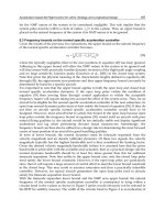
From Tables 3 and 4 one may observe that the model FO4 gives the smallest total error. This
is due to the fact that two FO terms are present in the model structure, allowing both a
decrease and increase in values of the impedance with frequency. The FO2 model is the
most commonly employed in clinical studies, with similar errors for the imaginary part, but
higher error in the real part of the impedance than the FO4 model. The underlying reason is
that the model can only capture a decrease in real part values of the impedance with
frequency, whereas some patients may present an increase. As an example, figure 4 presents
such a case, where one can visually compare the performance of the FO2 and FO4 models.

0 10 20 30 40 50
-0.05
0
0.05
0.1
0.15
0.2
Frequency (Hz)
Complex Impedance (kPa s/L)
Real Part
Imaginary
Part
0 10 20 30 40 50
-0.05
0
0.05
0.1
0.15
0.2
Frequency (Hz)
Complex Impedance (kPa s/L)
Real Part
Imaginary
Part


Fig. 4. A healthy subject data evaluated with FO4 (left) and with FO2 (right); continuous
lines denote the measured impedance and dashed lines denote the identified impedance.
1 2

0
0.5
1
1.5
2
2.5
3
3.5
Tissue damping G (kPa/l)
1 2
0
0.5
1
1.5
2
2.5
3
3.5
Tissue damping G (kPa/l)

Fig. 5. Tissue damping G (kPa/l) with FO2, p<3e
-5
(left) and with FO4, p<1e
-8
(right); 1:
Healthy subjects and 2: COPD patients.

1 2
0
2

4
6
8
10
Tissue elastance H (kPa/l)
1 2
0
2
4
6
8
10
Tissue elastance H (kPa/l)

Fig. 6. Tissue elastance H (kPa/l) with FO2, p<0.0012 (left) and with FO4, p<0.0004 (right); 1:
Healthy subjects and 2: COPD patients.

Recent Advances in Biomedical Engineering390

1 2
0
0.5
1
1.5
2
2.5
histeresitivity
1 2
0
0.5

1
1.5
2
2.5
histeresivity


Fig. 7. Tissue hysteresivity η with FO2, p<0.0012 (left) and with FO4, p<0.0004 (right); 1:
Healthy subjects and 2: COPD patients.

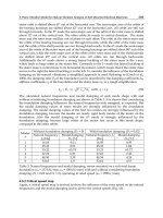
Figures 5, 6 and 7 depict the boxplots for the FO2 and FO4 for the tissue damping G, tissue
elastance H and histeresivity η. Due to the fact that FO2 has higher errors in fitting the
impedance values, the results are no further discussed. Although a similarity exists between
the values given by the two models, the discussion will be focused on the results obtained
using FO4.
Because FO are natural solutions in dielectric materials, it is interesting to look at the
permittivity property of respiratory tissues. In electric engineering, it is common to relate
permittivity to a material's ability to transmit (or permit) an electric field. By electrical
analogy, changes in trans-respiratory pressure relate to voltage difference, and changes in
air-flow relate to electrical current flows. When analyzing the permittivity index, one may
refer to an increased permittivity when the same amount of air-displacement is achieved
with smaller pressure difference. In other words, the hysteresivity coefficient incorporates
this property for the capacitor, that is, the COPD group has an increased capacitance,
justified by the pathology of the disease. Many alveolar walls are lost by emphysematous
lung destruction, the lungs become so loose and floppy that a small change in pressure is
enough to maintain a large volume, thus the lungs in COPD are highly compliant (elastic)
(Barnes, 2000; Hogg, 2004; Derom et al., 2007). The complex permittivity has a real part,
related to the stored energy within the medium and an imaginary part related to the
dissipation (or loss) of energy within the medium. The imaginary part of permittivity
corresponds to:

sin
2
L



 

 
 

(15)

If the values are positive, (15) denotes the absorption loss. In COPD, due to the sparseness of
the lung tissue, the air-flow in the alveoli is low, thus a low level of energy absorption is
observed in figure 8. In healthy subjects, due to increased alveolar surface, higher levels of
energy absorption are present, thus increased permittivity.

1 2
0.005
0.01
0.015
0.02
0.025
0.03
0.035
0.04
0.045
permitivity (kPa s²/l)

1 2
0.005
0.01
0.015
0.02
0.025
0.03
0.035
0.04
0.045
Permitivity (kPa s²/l)

Fig. 8. Boxplots for the computed permittivity index ε in the FO2, p<0.0081 (left) and in FO4,
p<0.0002 (right), in the two groups; 1: Healthy subjects and 2: COPD patients.

Another significant observation is that in general, FO4 identified more statistically
significant model parameter values than FO2. In figures 5-7 FO4 parameters had identified
similar variations between healthy and COPD groups. However, in figure 8, one can
observe that FO4 identified a more realistic variation between healthy and COPD groups,
i.e. a decreased permitivity index in COPD than in healthy.

6. Discussion
Tissue destruction (emphysema, COPD) and changes in air-space size and tissue elasticity
are matched with changes in model parameters when compared to the healthy group. The
physiological effects of chronic emphysema are extremely varied, depending on the severity
of the disease and on the relative degree of bronchiolar obstruction versus lung
parenchymal destruction (Barnes, 2000). Firstly, the bronchiolar obstruction greatly
increases airway resistance and results in increased work of breathing. It is especially
difficult for the person to move air through the bronchioles during expiration because the
compressive force on the outside of the lung not only compresses the alveoli but also

compresses the bronchioles, which further increase their resistance to expiration. This might
explain the decreased values for inertance (air mass acceleration), captured by the values of
L in the FO4. Secondly, the marked loss of lung parenchyma greatly decreases the elastin
cross-links, resulting in loss of attachments (Hogg, 2004). The latter can be directly related to
the fractional-order of compliance, which generally expresses the capability of a medium to
propagate mechanical properties (Suki et al., 1994).
The damping factor is a material parameter reflecting the capacity for energy absorption. In
materials similar to polymers, as lung tissue properties are very much alike polymers,
damping is mostly caused by viscoelasticity, i.e. the strain response lagging behind the
applied stresses (Suki et al., 1994;1997). In both FO models, the exponent β governs the
degree of the frequency dependence of tissue resistance and tissue elastance. The increased
lung elastance 1/C (stiffness) in COPD results in higher values of tissue damping and tissue
elastance, as observed in Figures 5 and 6. The loss of lung parenchyma (empty spaced lung),
consisting of collagen and elastin, both of which are responsible for characterizing lung
elasticity, is the leading cause of increased elastance in COPD. The hysteresivity coefficient η
Fractional-Order Models for the Input Impedance of the Respiratory System 391

1 2
0
0.5
1
1.5
2
2.5
histeresitivity
1 2
0
0.5
1
1.5

2
2.5
histeresivity


Fig. 7. Tissue hysteresivity η with FO2, p<0.0012 (left) and with FO4, p<0.0004 (right); 1:
Healthy subjects and 2: COPD patients.

Figures 5, 6 and 7 depict the boxplots for the FO2 and FO4 for the tissue damping G, tissue
elastance H and histeresivity η. Due to the fact that FO2 has higher errors in fitting the
impedance values, the results are no further discussed. Although a similarity exists between
the values given by the two models, the discussion will be focused on the results obtained
using FO4.
Because FO are natural solutions in dielectric materials, it is interesting to look at the
permittivity property of respiratory tissues. In electric engineering, it is common to relate
permittivity to a material's ability to transmit (or permit) an electric field. By electrical
analogy, changes in trans-respiratory pressure relate to voltage difference, and changes in
air-flow relate to electrical current flows. When analyzing the permittivity index, one may
refer to an increased permittivity when the same amount of air-displacement is achieved
with smaller pressure difference. In other words, the hysteresivity coefficient incorporates
this property for the capacitor, that is, the COPD group has an increased capacitance,
justified by the pathology of the disease. Many alveolar walls are lost by emphysematous
lung destruction, the lungs become so loose and floppy that a small change in pressure is
enough to maintain a large volume, thus the lungs in COPD are highly compliant (elastic)
(Barnes, 2000; Hogg, 2004; Derom et al., 2007). The complex permittivity has a real part,
related to the stored energy within the medium and an imaginary part related to the
dissipation (or loss) of energy within the medium. The imaginary part of permittivity
corresponds to:

sin

2
L



 

 
 

(15)

If the values are positive, (15) denotes the absorption loss. In COPD, due to the sparseness of
the lung tissue, the air-flow in the alveoli is low, thus a low level of energy absorption is
observed in figure 8. In healthy subjects, due to increased alveolar surface, higher levels of
energy absorption are present, thus increased permittivity.

1 2
0.005
0.01
0.015
0.02
0.025
0.03
0.035
0.04
0.045
permitivity (kPa s²/l)
1 2
0.005

0.01
0.015
0.02
0.025
0.03
0.035
0.04
0.045
Permitivity (kPa s²/l)

Fig. 8. Boxplots for the computed permittivity index ε in the FO2, p<0.0081 (left) and in FO4,
p<0.0002 (right), in the two groups; 1: Healthy subjects and 2: COPD patients.

Another significant observation is that in general, FO4 identified more statistically
significant model parameter values than FO2. In figures 5-7 FO4 parameters had identified
similar variations between healthy and COPD groups. However, in figure 8, one can
observe that FO4 identified a more realistic variation between healthy and COPD groups,
i.e. a decreased permitivity index in COPD than in healthy.

6. Discussion
Tissue destruction (emphysema, COPD) and changes in air-space size and tissue elasticity
are matched with changes in model parameters when compared to the healthy group. The
physiological effects of chronic emphysema are extremely varied, depending on the severity
of the disease and on the relative degree of bronchiolar obstruction versus lung
parenchymal destruction (Barnes, 2000). Firstly, the bronchiolar obstruction greatly
increases airway resistance and results in increased work of breathing. It is especially
difficult for the person to move air through the bronchioles during expiration because the
compressive force on the outside of the lung not only compresses the alveoli but also
compresses the bronchioles, which further increase their resistance to expiration. This might
explain the decreased values for inertance (air mass acceleration), captured by the values of

L in the FO4. Secondly, the marked loss of lung parenchyma greatly decreases the elastin
cross-links, resulting in loss of attachments (Hogg, 2004). The latter can be directly related to
the fractional-order of compliance, which generally expresses the capability of a medium to
propagate mechanical properties (Suki et al., 1994).
The damping factor is a material parameter reflecting the capacity for energy absorption. In
materials similar to polymers, as lung tissue properties are very much alike polymers,
damping is mostly caused by viscoelasticity, i.e. the strain response lagging behind the
applied stresses (Suki et al., 1994;1997). In both FO models, the exponent β governs the
degree of the frequency dependence of tissue resistance and tissue elastance. The increased
lung elastance 1/C (stiffness) in COPD results in higher values of tissue damping and tissue
elastance, as observed in Figures 5 and 6. The loss of lung parenchyma (empty spaced lung),
consisting of collagen and elastin, both of which are responsible for characterizing lung
elasticity, is the leading cause of increased elastance in COPD. The hysteresivity coefficient η
Recent Advances in Biomedical Engineering392

introduced in (Fredberg & Stamenovic, 1989) is G/H in this model representation. Given the
results observed in Figure 7, it is possible to distinguish between tissue changes from
healthy to COPD case. Since pathology of COPD involves significant variations between
inspiratory and expiratory air-flow, an increase in the hysteresivity coefficient η reflects
increased inhomogeneities and structural changes in the lungs.
It is difficult to provide a fair comparison between the values reported in this study and the
ones reported previously for tissue damping and elastance. Firstly, such studies have been
previously performed from excised lung measurements and invasive procedures (Suki et al.
1997; Brewer et al., 2003; Ito et al., 2007), which related these coefficients with transfer
impedance instead of input impedance. The measurement location is therefore important to
determine mechanical properties of lungs. The data reported in our study, has been derived
from non-invasive measurements at the mouth of the patients, therefore including upper
airway properties. Secondly, the previously reported
studies were made either on animal
data (Hantos et al., 1992a;1992b; Brewer et al., 2003; Ito et al., 2007), either on other lung

pathologies (Kaczka et al., 1999).
Another interesting aspect to note is that in the normal lung, the airways and lung
parenchyma are interdependent, with airway caliber monotonically increasing with lung
volume. In emphysematous lung, the caliber of small airways changes less than in the
normal lung (defining compliant properties) and peripheral airway resistance may increase
with increasing lung volume. At this point, the notion of space competition has been
introduced (Hogg, 2004), hypothesizing that enlarged emphysematous air spaces would
compress the adjacent small airways, according to a nonlinear behavior. Therefore, the
compression would be significantly higher at higher volumes rather than at low volumes,
resulting in blunting or even reversing the airway caliber changes during lung inflation.
This mechanism would therefore explain the significantly marked changes in model
parameters in tissue hysteresivity depicted in figure 7. It would be interesting to notice that
since small airway walls are collapsing, resulting in limited peripheral flow, it also leads to a
reduction of airway depths. A correlation between such airway depths reduction in the
diseased lung and model’s non-integer orders might give insight on the progress of the
disease in the lung.
The main limitation of the present study is that both model structures and their
corresponding parameter values are valid strictly within the specified frequency interval 4-
48Hz. Nonetheless, since only one resonant frequency is measured and is the closest to the
nominal breathing frequencies of the respiratory system, we do not seek to develop model
structures valid over larger frequency range. Moreover, it has been previously shown that
one model cannot capture the respiratory impedance over frequency intervals which
include more than one resonant frequency (Farré et al., 1989). A second limitation arises
from the parameters of the constant-phase models. The fractional-order operators are
difficult to handle numerically. The concept of modeling using non-integer order Laplace
(e.g.
1
,s
s



) is rather new in practical applications and has not reached the maturity of
integer-order system modeling. This concept has been borrowed from mathematics and
chemistry applications to model biological signals and systems only very recently. Advances
in technology and computation have enabled this topic in the latter decennia and it has
captured the interest of researchers. Although the parameters are intuitively related to

pathophysiology of respiratory mechanics, the structural interpretation of the fractional-
orders is in its early age.
Viscoelastic properties in lung parenchyma has been assessed in both animal and human
tissue strips (Suki et al., 1994) and correlated to fractional-order terms. A relation between
these fractional-orders and structural changes in airways and lung tissue has not been found
(e.g. airway remodeling). In this line of thought, the mechanical properties of resistance,
inertance and compliance have been derived from airway geometry and morphology (i.e.
airway radius, thickness, cartilage percent, length, etc) (Ionescu et al., 2009b). These
parameters have been employed in a recurrent structure of healthy lungs using analogue
representation of ladder networks (Ionescu et al., 2009d). In the latter contribution, the
appearance of a phase-lock (phase-constancy) is shown, supporting the argument that it
represents an intrinsic property (Oustaloup, 1995). Its correlation to changes in airway
morphology is an ongoing research matter. Experimental studies on various groups of
patients (e.g. asthma versus COPD) to investigate a possible classification strategy for the
parameters of this proposed model between various degrees of airway obstruction and lung
abnormalities may also offer interesting information upon the sensitivity of model
parameters.

7. Conclusions
This chapter presents a short overview on the properties of lung parenchyma in relation to
fractional order models for respiratory input impedance. Based on available model
structures from literature and our recent investigations, four fractional order models are
compared on two sets of impedance data: healthy and COPD (Chronic Obstructive

Pulmonary Disease). The results show that the two models broadly used in the clinical
studies and reported in the specialized literature are suitable for frequencies lower than
15Hz. However, when a higher range of frequencies is envisaged, two fractional orders in
the model structure are necessary, in order to capture the frequency dependence of the real
part in the complex respiratory impedance. Since the real part may both decrease and
increase within the evaluated frequency interval, there is need for both fractional order
derivative and fractional order integral parameters.
The multi-fractal model proposed in this chapter provides statistically significant values
between the healthy and COPD groups. Further investigations are planned in order to
evaluate if the model is able to discriminate between various pathologies (e.g. asthma, cystic
fibrosis and COPD).

Acknowledgements
C. Ionescu gratefully acknowledges the students who volunteered to perform lung function
testing in our laboratory, and the technical assistance provided at University of
Pharmacology and Medicine -“Leon Daniello” Cluj, Romania. This work was financially
supported by the UGent-BOF grant nr. B/07380/02.

Fractional-Order Models for the Input Impedance of the Respiratory System 393

introduced in (Fredberg & Stamenovic, 1989) is G/H in this model representation. Given the
results observed in Figure 7, it is possible to distinguish between tissue changes from
healthy to COPD case. Since pathology of COPD involves significant variations between
inspiratory and expiratory air-flow, an increase in the hysteresivity coefficient η reflects
increased inhomogeneities and structural changes in the lungs.
It is difficult to provide a fair comparison between the values reported in this study and the
ones reported previously for tissue damping and elastance. Firstly, such studies have been
previously performed from excised lung measurements and invasive procedures (Suki et al.
1997; Brewer et al., 2003; Ito et al., 2007), which related these coefficients with transfer
impedance instead of input impedance. The measurement location is therefore important to

determine mechanical properties of lungs. The data reported in our study, has been derived
from non-invasive measurements at the mouth of the patients, therefore including upper
airway properties. Secondly, the previously reported
studies were made either on animal
data (Hantos et al., 1992a;1992b; Brewer et al., 2003; Ito et al., 2007), either on other lung
pathologies (Kaczka et al., 1999).
Another interesting aspect to note is that in the normal lung, the airways and lung
parenchyma are interdependent, with airway caliber monotonically increasing with lung
volume. In emphysematous lung, the caliber of small airways changes less than in the
normal lung (defining compliant properties) and peripheral airway resistance may increase
with increasing lung volume. At this point, the notion of space competition has been
introduced (Hogg, 2004), hypothesizing that enlarged emphysematous air spaces would
compress the adjacent small airways, according to a nonlinear behavior. Therefore, the
compression would be significantly higher at higher volumes rather than at low volumes,
resulting in blunting or even reversing the airway caliber changes during lung inflation.
This mechanism would therefore explain the significantly marked changes in model
parameters in tissue hysteresivity depicted in figure 7. It would be interesting to notice that
since small airway walls are collapsing, resulting in limited peripheral flow, it also leads to a
reduction of airway depths. A correlation between such airway depths reduction in the
diseased lung and model’s non-integer orders might give insight on the progress of the
disease in the lung.
The main limitation of the present study is that both model structures and their
corresponding parameter values are valid strictly within the specified frequency interval 4-
48Hz. Nonetheless, since only one resonant frequency is measured and is the closest to the
nominal breathing frequencies of the respiratory system, we do not seek to develop model
structures valid over larger frequency range. Moreover, it has been previously shown that
one model cannot capture the respiratory impedance over frequency intervals which
include more than one resonant frequency (Farré et al., 1989). A second limitation arises
from the parameters of the constant-phase models. The fractional-order operators are
difficult to handle numerically. The concept of modeling using non-integer order Laplace

(e.g.
1
,s
s


) is rather new in practical applications and has not reached the maturity of
integer-order system modeling. This concept has been borrowed from mathematics and
chemistry applications to model biological signals and systems only very recently. Advances
in technology and computation have enabled this topic in the latter decennia and it has
captured the interest of researchers. Although the parameters are intuitively related to

pathophysiology of respiratory mechanics, the structural interpretation of the fractional-
orders is in its early age.
Viscoelastic properties in lung parenchyma has been assessed in both animal and human
tissue strips (Suki et al., 1994) and correlated to fractional-order terms. A relation between
these fractional-orders and structural changes in airways and lung tissue has not been found
(e.g. airway remodeling). In this line of thought, the mechanical properties of resistance,
inertance and compliance have been derived from airway geometry and morphology (i.e.
airway radius, thickness, cartilage percent, length, etc) (Ionescu et al., 2009b). These
parameters have been employed in a recurrent structure of healthy lungs using analogue
representation of ladder networks (Ionescu et al., 2009d). In the latter contribution, the
appearance of a phase-lock (phase-constancy) is shown, supporting the argument that it
represents an intrinsic property (Oustaloup, 1995). Its correlation to changes in airway
morphology is an ongoing research matter. Experimental studies on various groups of
patients (e.g. asthma versus COPD) to investigate a possible classification strategy for the
parameters of this proposed model between various degrees of airway obstruction and lung
abnormalities may also offer interesting information upon the sensitivity of model
parameters.

7. Conclusions
This chapter presents a short overview on the properties of lung parenchyma in relation to
fractional order models for respiratory input impedance. Based on available model
structures from literature and our recent investigations, four fractional order models are
compared on two sets of impedance data: healthy and COPD (Chronic Obstructive
Pulmonary Disease). The results show that the two models broadly used in the clinical
studies and reported in the specialized literature are suitable for frequencies lower than
15Hz. However, when a higher range of frequencies is envisaged, two fractional orders in
the model structure are necessary, in order to capture the frequency dependence of the real
part in the complex respiratory impedance. Since the real part may both decrease and
increase within the evaluated frequency interval, there is need for both fractional order
derivative and fractional order integral parameters.
The multi-fractal model proposed in this chapter provides statistically significant values
between the healthy and COPD groups. Further investigations are planned in order to
evaluate if the model is able to discriminate between various pathologies (e.g. asthma, cystic
fibrosis and COPD).

Acknowledgements
C. Ionescu gratefully acknowledges the students who volunteered to perform lung function
testing in our laboratory, and the technical assistance provided at University of
Pharmacology and Medicine -“Leon Daniello” Cluj, Romania. This work was financially
supported by the UGent-BOF grant nr. B/07380/02.

Recent Advances in Biomedical Engineering394

8. References
Adolfsson K., Enelund M., Olsson P., (2005), On the fractional order model of viscoelasticity,
Mechanics of Time-dependent materials, Springer, 9, 15–34
Barnes P.J., (2000), Chronic Obstructive Pulmonary Disease, NEJM Medical Progress, 343(4),
pp. 269-280

Birch M, MacLeod D, Levine M, (2001) An analogue instrument for the measurement of
respiratory impedance using the forced oscillation technique, Phys Meas, 22, pp.
323-339
Brewer K., Sakai H., Alencar A., Majumdar A., Arold S., Lutchen K., Ingenito E., Suki B.,
(2003), Lung and alveolar wall elastic and hysteretic behaviour in rats: effects of in
vivo elastase, J. Applied Physiology, 95(5), pp. 1926-1936
Craiem D., Armentano R., (2007) A fractional derivative model to describe arterial
viscoelasticity, Biorheology, 44, pp. 251—263
Coleman, T.F. and Y. Li, (1996), An interior trust region approach for nonlinear
minimization subject to bounds, SIAM Journal on Optimization, 6, 418-445
Daröczy B, Hantos Z, (1982) An improved forced oscillatory estimation of respiratory
impedance, Int J Bio-Medical Computing, 13, pp. 221-235
Derom E., Strandgarden K., Schelfhout V, Borgstrom L, Pauwels R. (2007), Lung deposition
and efficacy of inhaled formoterol in patients with moderate to severe COPD,
Respiratory Medicine, 101, pp. 1931-1941
Desager K, Buhr W, Willemen M, (1991), Measurement of total respiratory impedance in
infants by the forced oscillation technique, J Applied Physiology, 71, pp. 770-776
Desager D, Cauberghs M, Van De Woestijne K, (1997) Two point calibration procedure of
the forced oscillation technique, Med. Biol. Eng. Comput., 35, pp. 561-569
Diong B, Nazeran H., Nava P., Goldman M., (2007), Modelling human respiratory
impedance, IEEE Engineering in Medicine and Biology, 26(1), pp. 48-55
Eke, A., Herman, P., Kocsis, L., Kozak, L., (2002) Fractal characterization of complexity in
temporal physiological signals, Physiol Meas, 23, pp. R1-R38
Farré R, Peslin R, Oostveen E, Suki B, Duvivier C, Navajas D, (1989) Human respiratory
impedance from 8 to 256 Hz corrected for upper airway shunt, J Applied Physiology,
67, pp. 1973-1981
Franken H., Clement J, Caubergs M, Van de Woestijne K, (1981) Oscillating flow of a viscous
compressible fluid through a rigid tube, IEEE Trans Biomed Eng, 28, pp. 416-420
Fredberg J, Stamenovic D., (1989), On the imperfect elasticity of lung tissue, J. Applied
Physiology, 67:2408-2419

Gabrys, E., Rybaczuk, M., Kedzia, A., (2004) Fractal models of circulatory system.
Symmetrical and asymmetrical approach comparison, Chaos,Solitons and Fractals,
24(3), pp. 707-715
Govaerts E, Cauberghs M, Demedts M, Van de Woestijne K, (1994) Head generator versus
conventional technique in respiratory input impedance measuremenets, Eur Resp
Rev, 4, pp. 143-149
Hantos Z., Daroczy B., Klebniczki J., Dombos K, Nagy S., (1982) Parameter estimation of
transpulmonary mechanics by a nonlinear inertive model, J Appl Physiol, 52, pp 955-
-963
Hantos Z, Adamicza A, Govaerts E, Daroczy B., (1992) Mechanical Impedances of Lungs
and Chest Wall in the Cat, J. Applied Physiology, 73(2), pp. 427-433

Hogg J. C., (2004), Pathophysiology of airflow limitation in chronic obstructive pulmonary
disease, Lancet, 364, pp. 709-21
Ionescu, C. & De Keyser, R. (2008). Parametric models for characterizing the respiratory
input impedance. Journal of Medical Engineering & Technology, Taylor & Francis,
32(4), pp 315-324
Ionescu C., Desager K., De Keyser R., (2009a) Estimating respiratory mechanics with
constant-phase models in healthy lungs from forced oscillations measurements,
Studia Universitatis Vasile Goldis Life Sciences Series, 19(1), pp. 123-132
Ionescu C., Segers P., De Keyser R., (2009b) Mechanical properties of the respiratory system
derived from morphologic insight, IEEE Transactions on Biomedical Engineering,
April, 56(4), pp. 949-959
Ionescu C., De Keyser R., (2009c) Relations between Fractional Order Model Parameters and
Lung Pathology in Chronic Obstructive Pulmonary Disease, IEEE Transactions on
Biomedical Engineering, April, 56(4), pp. 978-987
Ionescu C., Oustaloup A., Levron F., De Keyser R., (2009d) “A model of the lungs based on
fractal geometrical and structural properties“, accepted contribution at the 15
th

IFAC Symposium on System Identification, St. Malo, France, 6-9 July 2009
Ionescu C, Tenreiro-Machado J., (in press), Mechanical properties and impedance model for
the branching network of the seiva system in the leaf of Hydrangea macrophylla,
accepted for publication in Nonlinear Dynamics
Ito S., Lutchen K., Suki B., (2007), “Effects of heterogeneities on the partitioning of airway
and tissue properties in mice”, J. Applied Physiology, 102(3), pp. 859-869
Kaczka D., Ingenito E., Israel E., Lutchen K., (1999), “Airway and lung tissue mechanics in
asthma: effects of albuterol”, Am J Respir Crit Care Med, 159, pp. 169-178
Jesus I, Tenreiro-Machado J, Cuhna B., (2008), Fractional electrical impedances in botanical
elements, Journal of Vibration and Control, 14, pp. 1389—1402
Losa G., Merlini D., Nonnenmacher T., Weibel E, (2005), Fractals in Biology and Medicine,
vol.IV, Birkhauser Verlag, Basel.
Mandelbrot B. (1983) The fractal geometry of nature, NY: Freeman &Co
Machado, Tenreiro J., Jesus I., (2004), Suggestion from the Past?, Fractional Calculus and
Applied Analysis, 7(4), pp. 403—407
Muntean I., Ionescu C., Nascu I., (2009) A simulator for the respiratory tree in healthy
subjects derived from continued fraction expansions, AIP Conference Proceedings vol.
1117: BICS 2008: Proceedings of the 1st International Conference on Bio-Inspired
Computational Methods Used for Difficult Problems Solving: Development of Intelligent
and Complex Systems, (Eds): B. Iantovics, Enachescu C., F. Filip, ISBN: 978-0-7354-
0654-4, pp. 225-231
Northrop R., (2002) Non-invasive measurements and devices for diagnosis, CRC Press
Oostveen, E., Macleod, D., Lorino, H., Farré, R., Hantos, Z., Desager, K., Marchal, F, (2003).
The forced oscillation technique in clinical practice: methodology,
recommendations and future developments, Eur Respir J, 22, pp 1026-1041
Oustaloup A. (1995) La derivation non-entière (in French), Hermes, Paris
Pasker H, Peeters M, Genet P, Nemery N, Van De Woestijne K., (1997) Short-term
Ventilatory Effects in Workers Exposed to Fumes Containing Zinc Oxide:
Comparison of Forced Oscillation Technique with Spirometry, Eur. Respir. J., 10: pp.
523-1529

Fractional-Order Models for the Input Impedance of the Respiratory System 395

8. References
Adolfsson K., Enelund M., Olsson P., (2005), On the fractional order model of viscoelasticity,
Mechanics of Time-dependent materials, Springer, 9, 15–34
Barnes P.J., (2000), Chronic Obstructive Pulmonary Disease, NEJM Medical Progress, 343(4),
pp. 269-280
Birch M, MacLeod D, Levine M, (2001) An analogue instrument for the measurement of
respiratory impedance using the forced oscillation technique, Phys Meas, 22, pp.
323-339
Brewer K., Sakai H., Alencar A., Majumdar A., Arold S., Lutchen K., Ingenito E., Suki B.,
(2003), Lung and alveolar wall elastic and hysteretic behaviour in rats: effects of in
vivo elastase, J. Applied Physiology, 95(5), pp. 1926-1936
Craiem D., Armentano R., (2007) A fractional derivative model to describe arterial
viscoelasticity, Biorheology, 44, pp. 251—263
Coleman, T.F. and Y. Li, (1996), An interior trust region approach for nonlinear
minimization subject to bounds, SIAM Journal on Optimization, 6, 418-445
Daröczy B, Hantos Z, (1982) An improved forced oscillatory estimation of respiratory
impedance, Int J Bio-Medical Computing, 13, pp. 221-235
Derom E., Strandgarden K., Schelfhout V, Borgstrom L, Pauwels R. (2007), Lung deposition
and efficacy of inhaled formoterol in patients with moderate to severe COPD,
Respiratory Medicine, 101, pp. 1931-1941
Desager K, Buhr W, Willemen M, (1991), Measurement of total respiratory impedance in
infants by the forced oscillation technique, J Applied Physiology, 71, pp. 770-776
Desager D, Cauberghs M, Van De Woestijne K, (1997) Two point calibration procedure of
the forced oscillation technique, Med. Biol. Eng. Comput., 35, pp. 561-569
Diong B, Nazeran H., Nava P., Goldman M., (2007), Modelling human respiratory
impedance, IEEE Engineering in Medicine and Biology, 26(1), pp. 48-55
Eke, A., Herman, P., Kocsis, L., Kozak, L., (2002) Fractal characterization of complexity in
temporal physiological signals, Physiol Meas, 23, pp. R1-R38

Farré R, Peslin R, Oostveen E, Suki B, Duvivier C, Navajas D, (1989) Human respiratory
impedance from 8 to 256 Hz corrected for upper airway shunt, J Applied Physiology,
67, pp. 1973-1981
Franken H., Clement J, Caubergs M, Van de Woestijne K, (1981) Oscillating flow of a viscous
compressible fluid through a rigid tube, IEEE Trans Biomed Eng, 28, pp. 416-420
Fredberg J, Stamenovic D., (1989), On the imperfect elasticity of lung tissue, J. Applied
Physiology, 67:2408-2419
Gabrys, E., Rybaczuk, M., Kedzia, A., (2004) Fractal models of circulatory system.
Symmetrical and asymmetrical approach comparison, Chaos,Solitons and Fractals,
24(3), pp. 707-715
Govaerts E, Cauberghs M, Demedts M, Van de Woestijne K, (1994) Head generator versus
conventional technique in respiratory input impedance measuremenets, Eur Resp
Rev, 4, pp. 143-149
Hantos Z., Daroczy B., Klebniczki J., Dombos K, Nagy S., (1982) Parameter estimation of
transpulmonary mechanics by a nonlinear inertive model, J Appl Physiol, 52, pp 955-
-963
Hantos Z, Adamicza A, Govaerts E, Daroczy B., (1992) Mechanical Impedances of Lungs
and Chest Wall in the Cat, J. Applied Physiology, 73(2), pp. 427-433

Hogg J. C., (2004), Pathophysiology of airflow limitation in chronic obstructive pulmonary
disease, Lancet, 364, pp. 709-21
Ionescu, C. & De Keyser, R. (2008). Parametric models for characterizing the respiratory
input impedance. Journal of Medical Engineering & Technology, Taylor & Francis,
32(4), pp 315-324
Ionescu C., Desager K., De Keyser R., (2009a) Estimating respiratory mechanics with
constant-phase models in healthy lungs from forced oscillations measurements,
Studia Universitatis Vasile Goldis Life Sciences Series, 19(1), pp. 123-132
Ionescu C., Segers P., De Keyser R., (2009b) Mechanical properties of the respiratory system
derived from morphologic insight, IEEE Transactions on Biomedical Engineering,
April, 56(4), pp. 949-959

Ionescu C., De Keyser R., (2009c) Relations between Fractional Order Model Parameters and
Lung Pathology in Chronic Obstructive Pulmonary Disease, IEEE Transactions on
Biomedical Engineering, April, 56(4), pp. 978-987
Ionescu C., Oustaloup A., Levron F., De Keyser R., (2009d) “A model of the lungs based on
fractal geometrical and structural properties“, accepted contribution at the 15
th

IFAC Symposium on System Identification, St. Malo, France, 6-9 July 2009
Ionescu C, Tenreiro-Machado J., (in press), Mechanical properties and impedance model for
the branching network of the seiva system in the leaf of Hydrangea macrophylla,
accepted for publication in Nonlinear Dynamics
Ito S., Lutchen K., Suki B., (2007), “Effects of heterogeneities on the partitioning of airway
and tissue properties in mice”, J. Applied Physiology, 102(3), pp. 859-869
Kaczka D., Ingenito E., Israel E., Lutchen K., (1999), “Airway and lung tissue mechanics in
asthma: effects of albuterol”, Am J Respir Crit Care Med, 159, pp. 169-178
Jesus I, Tenreiro-Machado J, Cuhna B., (2008), Fractional electrical impedances in botanical
elements, Journal of Vibration and Control, 14, pp. 1389—1402
Losa G., Merlini D., Nonnenmacher T., Weibel E, (2005), Fractals in Biology and Medicine,
vol.IV, Birkhauser Verlag, Basel.
Mandelbrot B. (1983) The fractal geometry of nature, NY: Freeman &Co
Machado, Tenreiro J., Jesus I., (2004), Suggestion from the Past?, Fractional Calculus and
Applied Analysis, 7(4), pp. 403—407
Muntean I., Ionescu C., Nascu I., (2009) A simulator for the respiratory tree in healthy
subjects derived from continued fraction expansions, AIP Conference Proceedings vol.
1117: BICS 2008: Proceedings of the 1st International Conference on Bio-Inspired
Computational Methods Used for Difficult Problems Solving: Development of Intelligent
and Complex Systems, (Eds): B. Iantovics, Enachescu C., F. Filip, ISBN: 978-0-7354-
0654-4, pp. 225-231
Northrop R., (2002) Non-invasive measurements and devices for diagnosis, CRC Press
Oostveen, E., Macleod, D., Lorino, H., Farré, R., Hantos, Z., Desager, K., Marchal, F, (2003).

The forced oscillation technique in clinical practice: methodology,
recommendations and future developments, Eur Respir J, 22, pp 1026-1041
Oustaloup A. (1995) La derivation non-entière (in French), Hermes, Paris
Pasker H, Peeters M, Genet P, Nemery N, Van De Woestijne K., (1997) Short-term
Ventilatory Effects in Workers Exposed to Fumes Containing Zinc Oxide:
Comparison of Forced Oscillation Technique with Spirometry, Eur. Respir. J., 10: pp.
523-1529
Recent Advances in Biomedical Engineering396

Podlubny, I. (1999). Fractional Differential Equations Mathematics in Sciences and
Engineering, vol. 198, Academic Press, ISBN 0125588402, New York.
Ramus-Serment M., Moreau X., Nouillant M, Oustaloup A., Levron F. (2002), Generalised
approach on fractional response of fractal networks, Chaos, Solitons and Fractals, 14,
pp. 479—488.
Suki, B., Barabasi, A.L., & Lutchen, K. (1994). Lung tissue viscoelasticity: a mathematical
framework and its molecular basis. J Applied Physiology, 76, pp. 2749-2759
Suki B., Yuan H., Zhang Q., Lutchen K., (1997) Partitioning of lung tissue response and
inhomogeneous airway constriction at the airway opening, J Applied Physiology, 82,
pp. 1349 1359
Van De Woestijne K, Desager K, Duiverman E, Marshall F, (1994) Recommendations for
measurement of respiratory input impedance by means of forced oscillation
technique, Eur Resp Rev, 4, pp. 235-237
Weibel, E.R. (2005). Mandelbrot’s fractals and the geometry of life: a tribute to Benoît
Mandelbrot on his 80
th
birthday, in Fractals in Biology and Medicine, vol IV, Eds: Losa
G., Merlini D., Nonnenmacher T., Weibel E.R., ISBN 9-783-76437-1722, Berlin:
Birkhaüser, pp 3-16
Modelling of Oscillometric Blood Pressure Monitor – from white to black box models 397
Modelling of Oscillometric Blood Pressure Monitor – from white to black

box models
Eduardo Pinheiro and Octavian Postolache
X

Modelling of Oscillometric Blood Pressure
Monitor – from white to black box models

Eduardo Pinheiro and Octavian Postolache
Instituto de Telecomunicações
Portugal

1. Introduction
Oscillometric blood pressure monitors (OBPMs) are a widespread medical device,
increasingly used both in domicile and clinical measurements of blood pressure, replacing
manual sphygmomanometers due to its simplicity of use and low price. A servo-based air
pump, an electronic valve and the inflatable cuff are the main components of an OBPM, the
nonlinear behaviour of the device emerges especially from this last element, in view of the
fact that the cuff’s expansion is constrained (Pinheiro, 2008).
The first sphygmomanometer developments and its final establishment, due to the works of
Samuel von Basch, Scipione Riva-Rocci and Nicolai Korotkoff, are over a century old, but
still are widely used by trained medical staff (Khan, 2006). In the Korotkoff sounds method,
a stethoscope is used to auscultate the sounds produced by the brachial artery while the
flow through it starts, after being occluded by the inflation of the cuff. The oscillometric
technique is an alternative method which examines the shape of the pressure oscillations
that the occluding cuff exhibits when the cuff‘s pressure diminishes from above systolic to
below diastolic blood pressure (Geddes et al., 1982), and in recent times it has been
increasingly applied (Pinheiro, 2008).
In the last decades, oscillometric blood pressure monitors have been employed as an
indirect measurement of blood pressure, but have not been subject of deep investigation,
and have been used as black-box systems, without explicit knowledge of their internal

dynamics and features. Bibliography in this field is limited, (Drzewiecki et al., 1993) studied
the cuff’s mechanics while (Ursino & Cristalli, 1996) have concerned with biomechanical
factors of the measurement, but both oblivious to the device’s behaviour and performance.
The equations that govern both wrist-OBPM and arm-OPBM behaviour are the same, but
wall compliances and other internal parameters assume diverse values, what may also
happen between different devices of the same type. The knowledge of the relations ruling
the internal dynamics of this instrument will help in the search for improvements in its
measurement accuracy and in the device design, given that electronic controllers may be
introduced to change the OBPM dynamics improving its sensibility. Moreover, since the
OBPM makes discrete measurements of the blood pressure, the understanding of the
device’s characteristics and dynamics may allow taking a leap towards continuous blood
pressure measurement using this inexpensive device.
21
Recent Advances in Biomedical Engineering398

Analyzing the OBPM, an insightful modelling effort is made to determine a white-box
model, describing the dynamics involved in the OBPM during cuff compression and
decompression and obtaining several non-ideal and nonlinear dynamics, using the results
available on servomotors (Ogata, 2001) and compressible flows (Shapiro, 1953), obtained
through electric, mechanic and thermodynamic principles. The approach taken was to
divide the OBPM in two subsystems, the electromechanical, which receives electrical supply
and outputs a torque in the crankshaft of the air pump, and the pneumatic subsystem,
which establishes the evolution of the cuff pressure, separating the compression and
decompression phases.
Subsequently blacker-box analysis is presented, in order to provide alternative models that
require only the observation of the air pump’s electric power dissipation, and pure
identification methods to estimate a multiple local model structure. In this last approach the
domain of operation was segmented in a number of operating regimes, identifying local
models for each regime and fusing them using different interpolation functions thus
providing better estimates and more flexibility in the system representation than a single

global model (Murray-Smith & Johansen, 1997).

2. White-box model
The main dynamics that characterize the OBPM behaviour are the air pump’s response to
the command voltage, the air propagation in the device and the inflatable cuff mechanics.

2.1 Electromechanical section
An armature controlled dc servomotor coupled to a crankshaft that manages two cylinders
that alternately compress the air are the components of the OBPM’s air pump. The
servomotor is controlled by V
a
, the voltage applied to its armature circuit, while a constant
magnetic flux is guaranteed. The armature-winding resistance is labelled R
a
, the inductance
L
a
, and the current i
a
, a depiction of the described command circuit is presented in Figure 1.



Fig. 1. Servomotor electrical control circuit

Due to the external magnetic field and the relative motion between the motor’s armature,
the back electromotive force, V
b
, appears. At constant magnetic flux V
b

is proportional to the
motor’s angular velocity, ω
m
, being related through the back electromotive force constant of
the motor, K
1
, and with ω
m
the derivative of θ
m
, the angular displacement of the shaft in the
motor, (1).


( )
1
( )
b m
V t K t
ω
=
(1)

The current evolution in the circuit, (2), is obtained with Kirchhoff’s laws.


( )
1
( )
( ) ( )

a
a a a m a
di t
L R i t K t V t
dt
ω
+ + =
(2)

The transformation from electrical to mechanical energy is done relating the torque τ to the
armature current, (3), where K
2
is the motor torque constant.


2
( ) ( )
a
t K i t
τ
=
(3)

Regarding the mechanical coupling to the crankshaft, it will be considered that the
servomotor and the crankshaft have moments of inertia J
m
and J
c
, rotate at angular velocities
ω

m
and ω
c
, and have angular displacements of θ
m
and θ
c
respectively. The shaft coupling, the
motor, and the crankshaft have non-homogeneous stiffness K
3
and viscous-friction b along
the shaft (x-axis), Figure 2.



Fig. 2. Mechanical representation of the servomotor coupling to the crankshaft.

The torsion is intrinsically displacement-dependent and the rotational dissipation is
velocity-dependent (Ljung & Glad, 1994), so, the equations of torque equilibrium will have
to consider the velocity and stiffness in every point of the shaft to compute the torsion,
regarding the friction along the shaft. This was dealt computing the product of the mean
values of the friction and the angular velocity, which may be piecewise-defined functions. In
(4) the angular velocity is defined as a function of time and location in the shaft, ω(t,x), with
ω(t,m) matching ω
m
(t) and ω(t,c) matching ω
c
(t).

( )
( )
3
2
3
2
( ) ( , )
( )
( ) ( , ) ( )
( ) ( , )
( )
( ) ( , ) 0
c c
c
m m m
m
m
m m
m
c c c
c
c
b x dx t x dx
d t
J K x t x dx t
dt
c m
b x dx t x dx
d t
J K x t x dx

dt
c m
ω
ω
ω τ
ω
ω
ω
 
 
 
+ + =
 
 
−
 
 
 
 
 
+ + =
 
−
 
 
∫ ∫
∫
∫ ∫
∫
(4)

It should be noted that in the case of homogeneous rigidity the last term of the sum is
simplified (5) just considering the angular displacements difference between θ
m
and θ
c
.
Moreover, if the coupling between the inertias is perfectly inflexible, which is a good
approximation if K
3
is very high, this term disappears.
Modelling of Oscillometric Blood Pressure Monitor – from white to black box models 399

Analyzing the OBPM, an insightful modelling effort is made to determine a white-box
model, describing the dynamics involved in the OBPM during cuff compression and
decompression and obtaining several non-ideal and nonlinear dynamics, using the results
available on servomotors (Ogata, 2001) and compressible flows (Shapiro, 1953), obtained
through electric, mechanic and thermodynamic principles. The approach taken was to
divide the OBPM in two subsystems, the electromechanical, which receives electrical supply
and outputs a torque in the crankshaft of the air pump, and the pneumatic subsystem,
which establishes the evolution of the cuff pressure, separating the compression and
decompression phases.
Subsequently blacker-box analysis is presented, in order to provide alternative models that
require only the observation of the air pump’s electric power dissipation, and pure
identification methods to estimate a multiple local model structure. In this last approach the
domain of operation was segmented in a number of operating regimes, identifying local
models for each regime and fusing them using different interpolation functions thus
providing better estimates and more flexibility in the system representation than a single
global model (Murray-Smith & Johansen, 1997).

2. White-box model
The main dynamics that characterize the OBPM behaviour are the air pump’s response to
the command voltage, the air propagation in the device and the inflatable cuff mechanics.

2.1 Electromechanical section
An armature controlled dc servomotor coupled to a crankshaft that manages two cylinders
that alternately compress the air are the components of the OBPM’s air pump. The
servomotor is controlled by V
a
, the voltage applied to its armature circuit, while a constant
magnetic flux is guaranteed. The armature-winding resistance is labelled R
a
, the inductance
L
a
, and the current i
a
, a depiction of the described command circuit is presented in Figure 1.



Fig. 1. Servomotor electrical control circuit

Due to the external magnetic field and the relative motion between the motor’s armature,
the back electromotive force, V
b
, appears. At constant magnetic flux V
b
is proportional to the
motor’s angular velocity, ω

m
, being related through the back electromotive force constant of
the motor, K
1
, and with ω
m
the derivative of θ
m
, the angular displacement of the shaft in the
motor, (1).


( )
1
( )
b m
V t K t
ω
=
(1)

The current evolution in the circuit, (2), is obtained with Kirchhoff’s laws.


( )
1
( )
( ) ( )
a
a a a m a

di t
L R i t K t V t
dt
ω
+ + =
(2)

The transformation from electrical to mechanical energy is done relating the torque τ to the
armature current, (3), where K
2
is the motor torque constant.


2
( ) ( )
a
t K i t
τ
=
(3)

Regarding the mechanical coupling to the crankshaft, it will be considered that the
servomotor and the crankshaft have moments of inertia J
m
and J
c
, rotate at angular velocities
ω
m
and ω

c
, and have angular displacements of θ
m
and θ
c
respectively. The shaft coupling, the
motor, and the crankshaft have non-homogeneous stiffness K
3
and viscous-friction b along
the shaft (x-axis), Figure 2.



Fig. 2. Mechanical representation of the servomotor coupling to the crankshaft.

The torsion is intrinsically displacement-dependent and the rotational dissipation is
velocity-dependent (Ljung & Glad, 1994), so, the equations of torque equilibrium will have
to consider the velocity and stiffness in every point of the shaft to compute the torsion,
regarding the friction along the shaft. This was dealt computing the product of the mean
values of the friction and the angular velocity, which may be piecewise-defined functions. In
(4) the angular velocity is defined as a function of time and location in the shaft, ω(t,x), with
ω(t,m) matching ω
m
(t) and ω(t,c) matching ω
c
(t).


( )
( )

3
2
3
2
( ) ( , )
( )
( ) ( , ) ( )
( ) ( , )
( )
( ) ( , ) 0
c c
c
m m m
m
m
m m
m
c c c
c
c
b x dx t x dx
d t
J K x t x dx t
dt
c m
b x dx t x dx
d t
J K x t x dx
dt
c m

ω
ω
ω τ
ω
ω
ω
 
 
 
+ + =
 
 
−
 
 
 
 
 
+ + =
 
−
 
 
∫ ∫
∫
∫ ∫
∫
(4)

It should be noted that in the case of homogeneous rigidity the last term of the sum is

simplified (5) just considering the angular displacements difference between θ
m
and θ
c
.
Moreover, if the coupling between the inertias is perfectly inflexible, which is a good
approximation if K
3
is very high, this term disappears.
Recent Advances in Biomedical Engineering400


3 3
( ) ( , ) ( ) ( )
c
m c
m
K x t x dx K t t
ω θ θ
= −
 
 
∫
(5)

Considering that the friction is applied in a single spatial point (x = b) and that the rigidity is
homogeneous, the set of equations obtained, (4), is linearized to (6).


3

3 3
3
( )
( ) ( ) ( )
2
( )
( ) ( ) ( ) ( ) 0
2 2
( )
( ) ( ) 0
2
m
m m b
b
b m b c
c
c c b
d t K
J t t t
dt
d t K K
b t t t t
dt
d t K
J t t
dt
ω
θ θ τ
θ
θ θ θ θ

ω
θ θ
 
+ − =
 
 
 
 
 
+ − + − =
   
 
   
 
 
+ − =
 
 
 
 
(6)

2.2 Pneumatic section
The air pump output flows through a short piping system of circular cross section before
entering in the cuff. The cylinders’ output is generally composed of a number of orifices
with very narrow diameter for example, three orifices with 0.5 mm which are linked
through a minor connector to a plastic piping system, of about 5 mm internal diameter,
conducing to the cuff. The modelling approach taken considers one-dimensional adiabatic
flow, with friction in the ducts, regarding air as a perfect gas, and with the pneumatic
connections represented by a converging-diverging nozzle, since the chamber-orifices

passage is a contraction, succeed by a two-step expansion, first the passage to the pipes and
next the arrival at the cuff.
The assumption of air as a perfect gas means that the specific heat is supposed constant and
the relation
RT
p
M
ρ
=
, is considered valid, with R the ideal gas constant, p and T its
absolute pressure and temperature, M the gas molar mass and ρ its density. In view of the
fact that at temperatures below 282 ºC the error of considering the specific heat constant is
negligible, and that deviations from the perfect gas equation of state are also negligible at
pressures below 50 atmospheres, the perfect gas approximation is found reasonable,
(Shapiro, 1953).
The maximum velocity of the flow, v
max
, may be determined considering the equation for
adiabatic stagnation of a stream (7), where γ is the ratio of specific heats (isobaric over
isochoric) and R the air constant, making the absolute temperature T null. It should be
noticed that the deceleration’s reversibility is not important since the stagnation
temperature, T
0
, will be the same.

( )
0
2
1
v R T T

γ
γ
= −
−
(7)
Regarding the pressure, if the deceleration is irreversible the final pressure will be smaller
than the isentropic stagnation pressure, p
0
, which is function of the Mach number, M
a
, the
ratio of the flow velocity and the speed of sound, as seen in (8).


1
2
0
1
1
2
a
p p M
γ
γ
γ
−
 
−
 
= +

 
 
 
 
(8)

But these are very high limits, if one considers realistic γ, e.g. 1.4 of (Forster & Turney, 1986),
even for very low temperature increases, the maximum velocity easily ascends at sonic
values, which generates elevated stagnation pressures limits also.
Searching for tighter limits, it is possible to find the characteristics of the air pumps used in
these applications. For instance, Koge KPM14A has an inflation time, from 0 to 300 mmHg,
in a 100 cm
3
tank, of, about 7.5 seconds. Therefore, considering this inflation time
representative, the mean volumetric flow is 13.333
×
10
-6
m
3
s
-1
so, the mean air speed is
11.789 ms
-1
in the three output orifices of the compression chamber, with 0.6 mm of diameter
each. The most of the piping has 5 mm of internal diameter, reducing the mean speed to
0.170 ms
-1
.

The Reynolds number of the flow,
Re
vD
ρ
µ
=
, calculated in [20 ; 80] ºC range to compensate
heating of the fluid, considering air’s dynamic viscosity μ and density ρ, at these
temperatures, and the velocity v in both sections, with different diameter D, will cause the
Reynolds number to be between 282 and 392 in the small orifices, and between 41 and 57 in
the duct. Hence the Reynolds number is far from 2000, guaranteeing laminar flow in the
orifices, even if the effective instantaneous speed achieves five times the mean speed
calculated, and in the ducts even if the flow is 35 times faster.
Since the flow is laminar, the friction factor f may be calculated simply using
16
Re
f =
. The
use of the friction factor to represent the walls’ shear stress, τ
w
, according to
2
2
w
f
v
τ
ρ
=
, is

correct if the flow is steady, but, in cases of velocity profile changes, f represents only an
“apparent friction factor” since it also includes momentum-flux effects. In short pipes,
which is clearly the case of the OBPM, the average apparent friction factor rises, (Shapiro,
1953) and (Goldwater & Fincham, 1981).
The air is fed into the 5 mm pipes from the three orifices of the compression chamber by an
element of unimportant length, which will be assumed frictionless. Since the chamber leads
to three 0.6 mm orifices converging to a 1 mm element, which introduces the flow in the 5
mm pipes, the piping profile is converging-diverging.
In view of the fact that the velocity would have to rise almost 29 times to produce sonic flow
in the orifices, the flow is considered entirely subsonic, and this piece behaves as a
conventional Venturi tube, introducing some losses in the flow (Benedict, 1980), with the
flow rate being sensitive to the cuff pressure, what would not happen in the case of sonic or
supersonic flow, where shock waves are present (Shapiro, 1953).
The effect of wall friction on fluid properties, considering one-dimensional (dx) adiabatic
flow of a perfect gas in a duct with hydraulic diameter D and friction factor f, will rewrite
the perfect gas, Mach number, energy, momentum, mass conservation, friction coefficient
and isentropic stagnation pressure equations (Shapiro, 1953), creating the system of
equations (9). The hydraulic diameter D changes along dx, and these changes must also be
included in the model implementation.
Modelling of Oscillometric Blood Pressure Monitor – from white to black box models 401


3 3
( ) ( , ) ( ) ( )
c
m c
m
K x t x dx K t t
ω θ θ
= −

 
 
∫
(5)

Considering that the friction is applied in a single spatial point (x = b) and that the rigidity is
homogeneous, the set of equations obtained, (4), is linearized to (6).


3
3 3
3
( )
( ) ( ) ( )
2
( )
( ) ( ) ( ) ( ) 0
2 2
( )
( ) ( ) 0
2
m
m m b
b
b m b c
c
c c b
d t K
J t t t
dt

d t K K
b t t t t
dt
d t K
J t t
dt
ω
θ θ τ
θ
θ θ θ θ
ω
θ θ
 
+ − =
 
 
 
 
 
+ − + − =
   
 
   
 
 
+ − =
 
 
 
 

(6)

2.2 Pneumatic section
The air pump output flows through a short piping system of circular cross section before
entering in the cuff. The cylinders’ output is generally composed of a number of orifices
with very narrow diameter for example, three orifices with 0.5 mm which are linked
through a minor connector to a plastic piping system, of about 5 mm internal diameter,
conducing to the cuff. The modelling approach taken considers one-dimensional adiabatic
flow, with friction in the ducts, regarding air as a perfect gas, and with the pneumatic
connections represented by a converging-diverging nozzle, since the chamber-orifices
passage is a contraction, succeed by a two-step expansion, first the passage to the pipes and
next the arrival at the cuff.
The assumption of air as a perfect gas means that the specific heat is supposed constant and
the relation
RT
p
M
ρ
=
, is considered valid, with R the ideal gas constant, p and T its
absolute pressure and temperature, M the gas molar mass and ρ its density. In view of the
fact that at temperatures below 282 ºC the error of considering the specific heat constant is
negligible, and that deviations from the perfect gas equation of state are also negligible at
pressures below 50 atmospheres, the perfect gas approximation is found reasonable,
(Shapiro, 1953).
The maximum velocity of the flow, v
max
, may be determined considering the equation for
adiabatic stagnation of a stream (7), where γ is the ratio of specific heats (isobaric over
isochoric) and R the air constant, making the absolute temperature T null. It should be

noticed that the deceleration’s reversibility is not important since the stagnation
temperature, T
0
, will be the same.

( )
0
2
1
v R T T
γ
γ
= −
−
(7)
Regarding the pressure, if the deceleration is irreversible the final pressure will be smaller
than the isentropic stagnation pressure, p
0
, which is function of the Mach number, M
a
, the
ratio of the flow velocity and the speed of sound, as seen in (8).


1
2
0
1
1
2

a
p p M
γ
γ
γ
−
 
−
 
= +
 
 
 
 
(8)

But these are very high limits, if one considers realistic γ, e.g. 1.4 of (Forster & Turney, 1986),
even for very low temperature increases, the maximum velocity easily ascends at sonic
values, which generates elevated stagnation pressures limits also.
Searching for tighter limits, it is possible to find the characteristics of the air pumps used in
these applications. For instance, Koge KPM14A has an inflation time, from 0 to 300 mmHg,
in a 100 cm
3
tank, of, about 7.5 seconds. Therefore, considering this inflation time
representative, the mean volumetric flow is 13.333
×
10
-6
m
3

s
-1
so, the mean air speed is
11.789 ms
-1
in the three output orifices of the compression chamber, with 0.6 mm of diameter
each. The most of the piping has 5 mm of internal diameter, reducing the mean speed to
0.170 ms
-1
.
The Reynolds number of the flow,
Re
vD
ρ
µ
=
, calculated in [20 ; 80] ºC range to compensate
heating of the fluid, considering air’s dynamic viscosity μ and density ρ, at these
temperatures, and the velocity v in both sections, with different diameter D, will cause the
Reynolds number to be between 282 and 392 in the small orifices, and between 41 and 57 in
the duct. Hence the Reynolds number is far from 2000, guaranteeing laminar flow in the
orifices, even if the effective instantaneous speed achieves five times the mean speed
calculated, and in the ducts even if the flow is 35 times faster.
Since the flow is laminar, the friction factor f may be calculated simply using
16
Re
f =
. The
use of the friction factor to represent the walls’ shear stress, τ
w

, according to
2
2
w
f
v
τ
ρ
=
, is
correct if the flow is steady, but, in cases of velocity profile changes, f represents only an
“apparent friction factor” since it also includes momentum-flux effects. In short pipes,
which is clearly the case of the OBPM, the average apparent friction factor rises, (Shapiro,
1953) and (Goldwater & Fincham, 1981).
The air is fed into the 5 mm pipes from the three orifices of the compression chamber by an
element of unimportant length, which will be assumed frictionless. Since the chamber leads
to three 0.6 mm orifices converging to a 1 mm element, which introduces the flow in the 5
mm pipes, the piping profile is converging-diverging.
In view of the fact that the velocity would have to rise almost 29 times to produce sonic flow
in the orifices, the flow is considered entirely subsonic, and this piece behaves as a
conventional Venturi tube, introducing some losses in the flow (Benedict, 1980), with the
flow rate being sensitive to the cuff pressure, what would not happen in the case of sonic or
supersonic flow, where shock waves are present (Shapiro, 1953).
The effect of wall friction on fluid properties, considering one-dimensional (dx) adiabatic
flow of a perfect gas in a duct with hydraulic diameter D and friction factor f, will rewrite
the perfect gas, Mach number, energy, momentum, mass conservation, friction coefficient
and isentropic stagnation pressure equations (Shapiro, 1953), creating the system of
equations (9). The hydraulic diameter D changes along dx, and these changes must also be
included in the model implementation.
Recent Advances in Biomedical Engineering402

( )
( )
( )
( )
( )
( )
( )
( )
2 2
2
2 2
2
2
2
2
2
4
2
2
2
2
0
0
1 1
4
2 1
2 1
4

2 1
4
2 1
1
4
2 1
4
2 1
4
2
a a
a
a a
a
a
a
a
a
a
a
a
a
a
M M
dp
dx
f
p D
M
M M

dM
dx
f
D
M
M
M
dv dx
f
v D
M
M
dT dx
f
T D
M
M
d dx
f
D
M
dp
M
dx
f
p D
γ γ
γ γ
γ
γ γ

γ
ρ
ρ
γ
 
 
+ −
 
 
= −
 
−
 
 
 
+ −
 
 
=
 
−
 
 
 
=
 
 
−
 
 

−
 
= −
 
−
 
 
 
= −
 
−
 
 
 
= −
 
 
(9)

The inflatable cuff is an element whose mechanical performance is a determinant factor of
the OBPM’s response (Pinheiro, 2008). Due to the pressure-volume bond and since the
constrictions to the cuff expansion introduce additional dynamics in the OBPM behaviour,
the complete model must incorporate (10) the model of cuff’s volume evolution with the
pressure. It was followed (Ursino & Cristalli, 1996) line of thought, but disagreeing in some
particular aspects, since it was considered cuff pressure perfectly equivalent to arm outer
surface pressure, greatly reducing the number of biomechanical parameters involved (and
their natural discrepancies when changing the subject’s characteristics), and also, the ratio of
specific heats γ was not considered constant, opposing to other, (Forster & Turney, 1986)
and (Ursino & Cristalli, 1996), approaches.

1 1 1
1 1 1
1 1
c c
w
c w
c c
dq dp dp
C
q q
dt dt p p dt
p p
γ γ
γ γ
γ γ
− +
+
− =
+
(10)

In this equation, q represents the amount of air contained in the cuff, p
c
is the cuff pressure (p
after the total piping length) expressed in relative units, C
w
is the wall compliance, -p
w
is the

collapse pressure of the cuff internal wall (pressure at which the wall compliance goes
infinite).
Finally, having characterized both fluid and structure equations, to complete this fluid-
structure interaction model, coupling equations must be defined. One option is to consider
fluid velocity inversely dependent on the crankshaft’s inertia J
c
, or alternatively, to consider
that the velocity is dependent on the crankshaft’s angular displacement θ
c
.
This crankshaft-based coupling is justified taking into consideration the air pump operation
cycle. The crankshaft is bicylindrical and each revolution makes the cylinders compress

once, since its construction is symmetrical, each revolution is the execution of the same
movement cycle twice, and this cycle can be decomposed in forward (compression) and
backward (recovery) movements, thus, the high frequency pulsatile air flow may have its
velocity expressed depending only on θ
c
or J
c
, with an appropriate rational transformation.
The modelling exercise is now complete, in the following section a greyer approach to
subject is made, studying in more detail the relation of the crankshaft-related variables with
the cuff pressure.


2.3 Greyer view – crankshaft load via power dissipation
A simplified way of modelling the mechanic-pneumatic connection will be to consider that
all the dynamics of the flow and the inflatable cuff are manifested in the load of the
servomotor. This way of thinking has the advantage of being assessed quite easily, by

measuring the air pump’s power dissipation, or the servomotor’s vibrations using strain
gages (Schicker & Wegener, 2002), with the latter requiring quite intrusive adjustments in
the OBPM, while the first only requires secondary wire connections.
Given that the crankshaft operation cycle can be decomposed in two forward
(compressions) and two backward (recoveries) movements, the inertia J
c
may be expressed
has a function dependent of θ
c
, (11), to include the high-frequency dynamics previously
described. However, since the dominant effect is unquestionably the filling of the cuff, J
c

must be strongly bonded to the cuff pressure. Since it noticeable that the compression takes
approximately 3π/4 rad, and the decompression lasts for about π/4 rad, these are the key
crankshaft’s angular displacement values.


( )
( )
3 7
( ) sin 2 3 , 0, ,
4 4
( , )
3 7
( ) ( ) sin 2 3 2 , , ,2
4 4
comp c c
c c
m dec c c

J p
J p
J p J p
π π
θ θ π
θ
π π
θ π θ π π
 
   
∈ ∪
 
   
 
   
=
 
   
 
+ − ∈ ∪
   
 
   
 
(11)

The raise in J
c
due to the cylinders’ forward and backward movement is represented by the
terms J

comp
and J
dec
correspondingly. The backward movement of the cylinders will add less
inertia to J
c
than the compression movement, and it is intuitive to suppose that both J
comp
and
J
dec
will increase when the pressure in the cuff increases. Also, a minimum inertia J
m
is added
during decompression, since the inertia does not reduce to zero immediately after the
compression ends. Subsequent Figure 3 shows the crankshaft’s inertia estimative produced
by (11) considering one cycle with a J
comp
value of 0.15 kgm
2
, J
dec
valuing 0.025 kgm
2
, and J
m

0.045 kgm
2
.

Measurements made on a wrist-OBPM air pump, Koge KPM14A, registered an armature-
winding resistance value of 3.9376 Ω and an inductance of 1.5893 mH, using an Agilent
4236B LCR meter (Pinheiro, 2008). Therefore, the implementation of a power measurement
scheme based on a 0.111 Ω resistor i n series with the supply circuit is innocuous to the
OBPM’s normal operation. The voltage in this resistor was acquired using a National
Instruments DAQ Card 6024E data-acquisition board at a sampling rate of 100
kSamples/second. The power dissipation evolution obtained from these measurements is
shown in Figure 4.
Modelling of Oscillometric Blood Pressure Monitor – from white to black box models 403


( )
( )
( )
( )
( )
( )
( )
( )
2 2
2
2 2
2
2
2
2
2
4
2
2

2
2
0
0
1 1
4
2 1
2 1
4
2 1
4
2 1
1
4
2 1
4
2 1
4
2
a a
a
a a
a
a
a
a
a
a
a
a

a
a
M M
dp
dx
f
p D
M
M M
dM
dx
f
D
M
M
M
dv dx
f
v D
M
M
dT dx
f
T D
M
M
d dx
f
D
M

dp
M
dx
f
p D
γ γ
γ γ
γ
γ γ
γ
ρ
ρ
γ
 
 
+ −
 
 
= −
 
−
 
 
 
+ −
 
 
=
 
−

 
 
 
=
 
 
−
 
 
−
 
= −
 
−
 
 
 
= −
 
−
 
 
 
= −
 
 
(9)

The inflatable cuff is an element whose mechanical performance is a determinant factor of
the OBPM’s response (Pinheiro, 2008). Due to the pressure-volume bond and since the

constrictions to the cuff expansion introduce additional dynamics in the OBPM behaviour,
the complete model must incorporate (10) the model of cuff’s volume evolution with the
pressure. It was followed (Ursino & Cristalli, 1996) line of thought, but disagreeing in some
particular aspects, since it was considered cuff pressure perfectly equivalent to arm outer
surface pressure, greatly reducing the number of biomechanical parameters involved (and
their natural discrepancies when changing the subject’s characteristics), and also, the ratio of
specific heats γ was not considered constant, opposing to other, (Forster & Turney, 1986)
and (Ursino & Cristalli, 1996), approaches.


1 1 1
1 1 1
1 1
c c
w
c w
c c
dq dp dp
C
q q
dt dt p p dt
p p
γ γ
γ γ
γ γ
− +
+
− =
+
(10)

In this equation, q represents the amount of air contained in the cuff, p
c
is the cuff pressure (p
after the total piping length) expressed in relative units, C
w
is the wall compliance, -p
w
is the
collapse pressure of the cuff internal wall (pressure at which the wall compliance goes
infinite).
Finally, having characterized both fluid and structure equations, to complete this fluid-
structure interaction model, coupling equations must be defined. One option is to consider
fluid velocity inversely dependent on the crankshaft’s inertia J
c
, or alternatively, to consider
that the velocity is dependent on the crankshaft’s angular displacement θ
c
.
This crankshaft-based coupling is justified taking into consideration the air pump operation
cycle. The crankshaft is bicylindrical and each revolution makes the cylinders compress

once, since its construction is symmetrical, each revolution is the execution of the same
movement cycle twice, and this cycle can be decomposed in forward (compression) and
backward (recovery) movements, thus, the high frequency pulsatile air flow may have its
velocity expressed depending only on θ
c
or J
c
, with an appropriate rational transformation.

The modelling exercise is now complete, in the following section a greyer approach to
subject is made, studying in more detail the relation of the crankshaft-related variables with
the cuff pressure.


2.3 Greyer view – crankshaft load via power dissipation
A simplified way of modelling the mechanic-pneumatic connection will be to consider that
all the dynamics of the flow and the inflatable cuff are manifested in the load of the
servomotor. This way of thinking has the advantage of being assessed quite easily, by
measuring the air pump’s power dissipation, or the servomotor’s vibrations using strain
gages (Schicker & Wegener, 2002), with the latter requiring quite intrusive adjustments in
the OBPM, while the first only requires secondary wire connections.
Given that the crankshaft operation cycle can be decomposed in two forward
(compressions) and two backward (recoveries) movements, the inertia J
c
may be expressed
has a function dependent of θ
c
, (11), to include the high-frequency dynamics previously
described. However, since the dominant effect is unquestionably the filling of the cuff, J
c

must be strongly bonded to the cuff pressure. Since it noticeable that the compression takes
approximately 3π/4 rad, and the decompression lasts for about π/4 rad, these are the key
crankshaft’s angular displacement values.


( )
( )
3 7

( ) sin 2 3 , 0, ,
4 4
( , )
3 7
( ) ( ) sin 2 3 2 , , ,2
4 4
comp c c
c c
m dec c c
J p
J p
J p J p
π π
θ θ π
θ
π π
θ π θ π π
 
   
∈ ∪
 
   
 
   
=
 
   
 
+ − ∈ ∪
   

 
   
 
(11)

The raise in J
c
due to the cylinders’ forward and backward movement is represented by the
terms J
comp
and J
dec
correspondingly. The backward movement of the cylinders will add less
inertia to J
c
than the compression movement, and it is intuitive to suppose that both J
comp
and
J
dec
will increase when the pressure in the cuff increases. Also, a minimum inertia J
m
is added
during decompression, since the inertia does not reduce to zero immediately after the
compression ends. Subsequent Figure 3 shows the crankshaft’s inertia estimative produced
by (11) considering one cycle with a J
comp
value of 0.15 kgm
2
, J

dec
valuing 0.025 kgm
2
, and J
m

0.045 kgm
2
.
Measurements made on a wrist-OBPM air pump, Koge KPM14A, registered an armature-
winding resistance value of 3.9376 Ω and an inductance of 1.5893 mH, using an Agilent
4236B LCR meter (Pinheiro, 2008). Therefore, the implementation of a power measurement
scheme based on a 0.111 Ω resistor i n series with the supply circuit is innocuous to the
OBPM’s normal operation. The voltage in this resistor was acquired using a National
Instruments DAQ Card 6024E data-acquisition board at a sampling rate of 100
kSamples/second. The power dissipation evolution obtained from these measurements is
shown in Figure 4.
Recent Advances in Biomedical Engineering404



Fig. 3. Crankshaft inertia estimate characterization during one complete revolution, under
J
comp
, J
dec
, J
m
of 0.150, 0.025, and 0.045 kgm
2

.



Fig. 4. Power dissipation in the air pump during one complete revolution of the crankshaft.

The abrupt dissipated power decreases after the local maximums are due to the conclusion
of the forward and backward movements. The decompression conclusion practically leads
to a zero power situation, while the compression conclusion is seen in previous Figure 4 to
reduce the power to 50% of the maximum. The 50% proportion is approximately constant if
the cuff pressure is below 20 centimetres of mercury column (cmHg), which is the nominal
pressure range of OBPM’s cuff. This means that in inertia terms, (11), J
m
should be half of
max{J
comp
} calculated at the end of the compression.
The cuff pressure directly affects the terms J
comp
and J
dec
, since it is the variable ruling the
effort of the air pump in each compression. Noticing that it is most important to measure the
servomotor’s power dissipation evolution and this high-frequency dynamic is not so
significant, the curve in Figure 4 may be low-pass filtered in order to evaluate the power
evolution once the air pumping changes the cuff pressure, instead of analysing every pump
stroke.
To the acquisition hardware was added a Measurement Specialities 1451 pressure sensor,
and it was implemented digitally a 3
rd

order Butterworth low-pass filter with 30 Hz cut-off

frequency. The results obtained are shown in Figure 5, where it is seen the power
dissipation curves when compressing to the inflatable cuff, left, and to a constant volume
reservoir with about the same capacity, right.



Fig. 5. Air pump’s power dissipation dependence of cuff-pressure (blue) and approximating
curve (red), when the air pump output is connected to the cuff (left) and to a constant-
volume reservoir (right).

The air pump power dissipation, P, relation with the downstream pressure, p, was
approximated by a rational function, (12), with coefficient of determination, R
2
, of 0.984
when connected to the cuff and 0.967 when connected to the constant-volume reservoir, the
a normalized root mean square deviation of the approximations was 2.17% and 2.26%,
respectively. With these approximation functions, from the pressure measurements the
power dissipation is calculated.


4 3 2
4 3 2 1 0
0
( ) ( ) ( ) ( )
( )
( )
a p t a p t a p t a p t a
P t

p t b
+ + + +
=
+
(12)

The inertia of the crankshaft J
c
as been described as possible to be estimated from the power
dissipation, this makes sense given that the major portion of the crankshaft’s inertia is due to
the cuff pressure, and the power-pressure relation has been established in (12). Thus, it will
be assumed that low-pass filtering the crankshaft’s inertia in a 30 Hz 3
rd
order Butterworth
filter Ψ, makes it directly proportional to the power dissipation, (13), being K
4
the power-
inertia conversion constant.


( )
4
( ) ( )
c
J t K P tΨ =
(13)

Modelling of Oscillometric Blood Pressure Monitor – from white to black box models 405

Fig. 3. Crankshaft inertia estimate characterization during one complete revolution, under
J
comp
, J
dec
, J
m
of 0.150, 0.025, and 0.045 kgm
2
.



Fig. 4. Power dissipation in the air pump during one complete revolution of the crankshaft.

The abrupt dissipated power decreases after the local maximums are due to the conclusion
of the forward and backward movements. The decompression conclusion practically leads
to a zero power situation, while the compression conclusion is seen in previous Figure 4 to
reduce the power to 50% of the maximum. The 50% proportion is approximately constant if
the cuff pressure is below 20 centimetres of mercury column (cmHg), which is the nominal
pressure range of OBPM’s cuff. This means that in inertia terms, (11), J
m
should be half of
max{J
comp
} calculated at the end of the compression.
The cuff pressure directly affects the terms J
comp
and J

dec
, since it is the variable ruling the
effort of the air pump in each compression. Noticing that it is most important to measure the
servomotor’s power dissipation evolution and this high-frequency dynamic is not so
significant, the curve in Figure 4 may be low-pass filtered in order to evaluate the power
evolution once the air pumping changes the cuff pressure, instead of analysing every pump
stroke.
To the acquisition hardware was added a Measurement Specialities 1451 pressure sensor,
and it was implemented digitally a 3
rd
order Butterworth low-pass filter with 30 Hz cut-off

frequency. The results obtained are shown in Figure 5, where it is seen the power
dissipation curves when compressing to the inflatable cuff, left, and to a constant volume
reservoir with about the same capacity, right.



Fig. 5. Air pump’s power dissipation dependence of cuff-pressure (blue) and approximating
curve (red), when the air pump output is connected to the cuff (left) and to a constant-
volume reservoir (right).

The air pump power dissipation, P, relation with the downstream pressure, p, was
approximated by a rational function, (12), with coefficient of determination, R
2
, of 0.984
when connected to the cuff and 0.967 when connected to the constant-volume reservoir, the
a normalized root mean square deviation of the approximations was 2.17% and 2.26%,
respectively. With these approximation functions, from the pressure measurements the
power dissipation is calculated.

4 3 2
4 3 2 1 0
0
( ) ( ) ( ) ( )
( )
( )
a p t a p t a p t a p t a
P t
p t b
+ + + +
=
+
(12)

The inertia of the crankshaft J
c
as been described as possible to be estimated from the power
dissipation, this makes sense given that the major portion of the crankshaft’s inertia is due to
the cuff pressure, and the power-pressure relation has been established in (12). Thus, it will
be assumed that low-pass filtering the crankshaft’s inertia in a 30 Hz 3
rd
order Butterworth
filter Ψ, makes it directly proportional to the power dissipation, (13), being K
4
the power-
inertia conversion constant.

( )
4
( ) ( )
c
J t K P tΨ =
(13)

Recent Advances in Biomedical Engineering406

Aggregating the equations of the electromechanical section, with (12) and (13), and choosing
state vector X, defined in (14), it is assembled a greyer and simpler space-state model of the
OBPM.


( ) ( ), ( ), ( ), ( ), ( )
T
T
c c m m a
X t t t t t i t
θ ω θ ω
=
 
 
(14)

It should be noticed that since power is the product of i
a
the air pump’s current (state
variable) and V
a

the voltage applied (input variable), both pressure and inertia can be
estimated knowing only the power and applying (12) and (13) in that order.

2.4 Cuff decompression
The OBPM controls the air pump and the electronic valve in order to pressurize the cuff,
until blood flow is cut off, and afterwards slowly reduces the cuff pressure, stopping the
compression and letting the cuff’s permanent leakage take effect, only opening the electronic
valve to swiftly deplete the cuff when the blood pressure measurement is done. During the
period while the air pump is stopped and the valve is closed, it is also necessary to evaluate
the cuff pressure dynamic when the permanent leakage is the only influence.
In a constant-volume reservoir this dynamic is defined by an exponential decay, as seen in
(Lyung & Glad, 1994), in this case, due to the expandability of the cuff, other parameters
must infer in the exponential.
It were recorded twelve descents, by turning off the air pump at different pressures, p
off
,
from 9 to 20 cmHg, and then using the DAQ Card 6024E data-acquisition board at 1 kS/s to
record the pressure fall curve. It was verified that the cuff pressure had an exponential
decay,
( )
bt
p t ae
−
=
, and that the exponential function parameters, a and b, were dependent
on the pressure at which the inflation was stopped, p
0ff
, as presented in (15), with
corresponding coefficient of determination values of 0.980 and 0.877.

0.0732
1.126 3.35
0.3436
off
off
p
a p
b e
−
= −
 
 
 
= −
 
 
(15)

3. Black-box model
The main nonlinearities involved in the OBPM operation refer to the dynamics of the air
compression and flow, and the limitations to the cuff expansion. The black-box model
approach will define a single-input single-output relation between the voltage supply to the
OBPM’s air pump, V
a
, and the cuff pressure, p, applying system identification procedures
(Ljung, 1999).
The OBPM, in its normal operating cycle, keeps the electronic valve always closed, by
powering it, until cuff depletion is desired, and controls the air pump to compress the cuff
until blood stops flowing. To do this, a National Instruments USB-6008 multifunction I/O

board was used, with an acquisition rate and generation rate of 50 S/s, together with
appropriate circuitry to allow supervision of the device’s elements.

The identification procedure consisted of randomly deciding to power the air pump using
white noise, but keeping the pressure in a defined range to maintain the device in the
operating regime to be identified, thus in case of pressure range surpass the power was shut
down and vice versa.
It was found by experience that the command voltage should be updated at a rate lower
than the 50 S/s used to read the pressure sensor value, to permit the visualization of the
effects of the voltage change, and so it was used a 10 S/s output update rate.
Besides connecting the air piping output to the wrist inflatable cuff, the OBPM identification
tests were replied in the constant-volume reservoir, to observe the differences in the results
due to the reservoir expansion.

3.1 At 5 regimes
The inflatable cuff’s maximum nominal pressure is 19.5 cmHg, but, since an hypertensive
person may have a systolic blood pressure higher than this limit, the maximum pressure
considered was 22 cmHg, and the divisions were: [0 ; 6], ]6 ; 10], ]10 ; 14], ]14 ; 18] and ]18 ;
22] cmHg. These divisions arose from the analysis of the OBPM’s behaviour when inflating
the cuff, from which it was noticed that there are clearly different operating regimes,
corresponding to the pressure ranges specified.
The identification tests had 30 minutes of duration, with the first 15 being used to estimate
the models and the remaining to validate them. It were computed Output Error (OE),
Autoregressive Exogenous Variable (ARX), Autoregressive Moving Average Exogenous
Variable (ARMAX), and Box-Jenkins (BJ) models, using the formulation of (Lyung, 1999), of
3
rd
and 5
th
order (in all polynomials involved) without delay.

The fits of the various regimes were computed according to (16) (p
av
is the average pressure
and p
est
the estimated pressure), and respecting the cuff and the constant-volume reservoir,
are displayed in Table 1 and Table 2.


%
-
fit 100
est
av
p p
p p
= ×
−
(16)

Pressure
[cmHg ]
OE3 OE5 ARX3 ARX5 ARMAX3 ARMAX5 BJ3 BJ5
0-6
80.56 89.82 75.19 74.96 71.93 87.47 69.47 87.55
6-10
72.20 77.64 66.38 67.82 73.36 77.86 72.47 78.53
10-14
74.09 68.87 62.77 65.78 63.09 75.32 68.95 75.14
14-18

66.64 69.08 51.37 52.68 39.01 36.14 45.86 41.96
18-22
32.34 50.61 33.19 32.77 18.30 13.57 4.39 7.74

Table 1. Models’ fit evolution with the air pump output connected to the inflatable cuff

From these results it is seen that the 5
th
order OE is the fittest model (highest average,
μ=71.21, and lowest standard deviation, σ=14.33) with the 3
rd
order OE having the second
highest μ of 65.16, showing the appropriateness of this model type, as it considers the error
as white-noise, without estimating a noise model. The global μ is of 59.32 and σ of 25.63.

Modelling of Oscillometric Blood Pressure Monitor – from white to black box models 407

Aggregating the equations of the electromechanical section, with (12) and (13), and choosing
state vector X, defined in (14), it is assembled a greyer and simpler space-state model of the
OBPM.


( ) ( ), ( ), ( ), ( ), ( )
T
T
c c m m a
X t t t t t i t
θ ω θ ω
=
 

 
(14)

It should be noticed that since power is the product of i
a
the air pump’s current (state
variable) and V
a
the voltage applied (input variable), both pressure and inertia can be
estimated knowing only the power and applying (12) and (13) in that order.

2.4 Cuff decompression
The OBPM controls the air pump and the electronic valve in order to pressurize the cuff,
until blood flow is cut off, and afterwards slowly reduces the cuff pressure, stopping the
compression and letting the cuff’s permanent leakage take effect, only opening the electronic
valve to swiftly deplete the cuff when the blood pressure measurement is done. During the
period while the air pump is stopped and the valve is closed, it is also necessary to evaluate
the cuff pressure dynamic when the permanent leakage is the only influence.
In a constant-volume reservoir this dynamic is defined by an exponential decay, as seen in
(Lyung & Glad, 1994), in this case, due to the expandability of the cuff, other parameters
must infer in the exponential.
It were recorded twelve descents, by turning off the air pump at different pressures, p
off
,
from 9 to 20 cmHg, and then using the DAQ Card 6024E data-acquisition board at 1 kS/s to
record the pressure fall curve. It was verified that the cuff pressure had an exponential
decay,
( )
bt
p t ae

−
=
, and that the exponential function parameters, a and b, were dependent
on the pressure at which the inflation was stopped, p
0ff
, as presented in (15), with
corresponding coefficient of determination values of 0.980 and 0.877.


0.0732
1.126 3.35
0.3436
off
off
p
a p
b e
−
= −
 
 
 
= −
 
 
(15)

3. Black-box model
The main nonlinearities involved in the OBPM operation refer to the dynamics of the air
compression and flow, and the limitations to the cuff expansion. The black-box model

approach will define a single-input single-output relation between the voltage supply to the
OBPM’s air pump, V
a
, and the cuff pressure, p, applying system identification procedures
(Ljung, 1999).
The OBPM, in its normal operating cycle, keeps the electronic valve always closed, by
powering it, until cuff depletion is desired, and controls the air pump to compress the cuff
until blood stops flowing. To do this, a National Instruments USB-6008 multifunction I/O
board was used, with an acquisition rate and generation rate of 50 S/s, together with
appropriate circuitry to allow supervision of the device’s elements.

The identification procedure consisted of randomly deciding to power the air pump using
white noise, but keeping the pressure in a defined range to maintain the device in the
operating regime to be identified, thus in case of pressure range surpass the power was shut
down and vice versa.
It was found by experience that the command voltage should be updated at a rate lower
than the 50 S/s used to read the pressure sensor value, to permit the visualization of the
effects of the voltage change, and so it was used a 10 S/s output update rate.
Besides connecting the air piping output to the wrist inflatable cuff, the OBPM identification
tests were replied in the constant-volume reservoir, to observe the differences in the results
due to the reservoir expansion.

3.1 At 5 regimes
The inflatable cuff’s maximum nominal pressure is 19.5 cmHg, but, since an hypertensive
person may have a systolic blood pressure higher than this limit, the maximum pressure
considered was 22 cmHg, and the divisions were: [0 ; 6], ]6 ; 10], ]10 ; 14], ]14 ; 18] and ]18 ;
22] cmHg. These divisions arose from the analysis of the OBPM’s behaviour when inflating
the cuff, from which it was noticed that there are clearly different operating regimes,
corresponding to the pressure ranges specified.
The identification tests had 30 minutes of duration, with the first 15 being used to estimate

the models and the remaining to validate them. It were computed Output Error (OE),
Autoregressive Exogenous Variable (ARX), Autoregressive Moving Average Exogenous
Variable (ARMAX), and Box-Jenkins (BJ) models, using the formulation of (Lyung, 1999), of
3
rd
and 5
th
order (in all polynomials involved) without delay.
The fits of the various regimes were computed according to (16) (p
av
is the average pressure
and p
est
the estimated pressure), and respecting the cuff and the constant-volume reservoir,
are displayed in Table 1 and Table 2.


%
-
fit 100
est
av
p p
p p
= ×
−
(16)

Pressure
[cmHg ]

OE3 OE5 ARX3 ARX5 ARMAX3 ARMAX5 BJ3 BJ5
0-6
80.56 89.82 75.19 74.96 71.93 87.47 69.47 87.55
6-10
72.20 77.64 66.38 67.82 73.36 77.86 72.47 78.53
10-14
74.09 68.87 62.77 65.78 63.09 75.32 68.95 75.14
14-18
66.64 69.08 51.37 52.68 39.01 36.14 45.86 41.96
18-22
32.34 50.61 33.19 32.77 18.30 13.57 4.39 7.74

Table 1. Models’ fit evolution with the air pump output connected to the inflatable cuff

From these results it is seen that the 5
th
order OE is the fittest model (highest average,
μ=71.21, and lowest standard deviation, σ=14.33) with the 3
rd
order OE having the second
highest μ of 65.16, showing the appropriateness of this model type, as it considers the error
as white-noise, without estimating a noise model. The global μ is of 59.32 and σ of 25.63.

Recent Advances in Biomedical Engineering408

Pressure
[cmHg]
OE3 OE5 ARX3 ARX5 ARMAX3 ARMAX5 BJ3 BJ5
0-6
68.35 68.72 70.78 70.03 68.46 73.79 69.26 69.74

6-10
66.81 70.51 60.50 60.17 60.51 69.01 60.48 71.27
10-14
51.21 51.71 51.57 51.69 58.89 48.06 59.37 60.01
14-18
64.11 62.81 56.22 56.44 57.85 50.85 57.93 51.05
18-22
48.89 9.76 40.00 39.23 3.64 33.78 2.29 36.90

Table 2. Models’ fit evolution with the air pump output connected to the constant-volume
reservoir

The results presented in Table 2 show the 3
rd
order OE as being the fittest model (highest
μ=59.87, and lowest σ=9.13) while the 5
th
order BJ has the second highest μ of 57.79. The
global μ decreases 9.44% to 53.71 and σ decreases 9.05% to 23.31, implying that although the
fits were lower in average, their dispersion also diminished, given the general improvement
in the two highest pressure regimes.
It is evident that for both cases the last regime ]18 ; 22] cmHg is very difficult to represent
using these models, since in the cuff tests the average fit for this regime was of 24.10 and in
the reservoir 22.58. This regime is partially above the maximum nominal pressure, and the
OBPM’s dynamic is not homogeneous inside this pressure range, generating the poorest fit
of all regimes.

3.2 At 22 regimes
The pressure range was divided in intervals with 1 cmHg of span, after the first which is [0 ;
2] cmHg, and the tests duration was reduced to 10 minutes. In subsequent Figure 6 and

Figure 7 it is displayed the fits evolution, the first presents the results with air pump output
connected to the cuff and the latter when connected to the constant-volume reservoir.



Fig. 6. Models’ fit evolution when the air pump output is connected to the cuff

From these results it is seen that the 3
rd
order OE is the fittest model (highest average,
μ=70.60, and lowest standard deviation, σ=6.88) with the 5
th
order OE having the second
highest μ, 64.14. Such results show the suitability of this particular model type, as all other
models have worse behaviour, namely the ARX models, with average fit below 30.
Comparing with the 5 models approach, the global μ is of 48.61, a decrease of 18.06%, and σ
of 26.62, a 3.84% increase.



Fig. 7. Models’ fit evolution when the air pump output is connected to the constant-volume
reservoir

As happened with the cuff tests, the 3
rd
order OE is again the fittest model (μ
OE3
=66.64,
σ
OE3

=7.52) while the 5
th
order OE is very near (μ
OE5
=65.06). The global μ decreases 5.29% to
50.88 and σ increases 9.05% to 26.79 regarding the 5 models approach. Regarding the
compression to the cuff with 22 models, global μ has increased 4.66% and global σ 0.66%.
It is discernible that for both cases the OE models have a regular fit, which does not decrease
much in the higher pressure regimes. Moreover, comparing the average fit of the models
that comprise the ]18 ; 22] cmHg range, to the fit of the corresponding 5-regimes model, the
division gains are evident.
Table 3 presents the fit increase for the three best models of the cuff and reservoir tests. The
fit increase is the difference from the average fit of the 22-regimes models to the fit of 5-
regimes model in the ]18:22] cmHg pressure range.

Model
OE3-cuff OE5-cuff BJ5-cuff OE3-res OE5-res BJ5-res
Fit increase [%]
31.80
8.01
50.69
11.39
47.55
-1.08
Table 3. Difference between the fit of the ]18:22] cmHg regime and the average fits of the
models that comprise this pressure range in the 22 divisions tests

Modelling of Oscillometric Blood Pressure Monitor – from white to black box models 409

Pressure

[cmHg]
OE3 OE5 ARX3 ARX5 ARMAX3 ARMAX5 BJ3 BJ5
0-6
68.35 68.72 70.78 70.03 68.46 73.79 69.26 69.74
6-10
66.81 70.51 60.50 60.17 60.51 69.01 60.48 71.27
10-14
51.21 51.71 51.57 51.69 58.89 48.06 59.37 60.01
14-18
64.11 62.81 56.22 56.44 57.85 50.85 57.93 51.05
18-22
48.89 9.76 40.00 39.23 3.64 33.78 2.29 36.90

Table 2. Models’ fit evolution with the air pump output connected to the constant-volume
reservoir

The results presented in Table 2 show the 3
rd
order OE as being the fittest model (highest
μ=59.87, and lowest σ=9.13) while the 5
th
order BJ has the second highest μ of 57.79. The
global μ decreases 9.44% to 53.71 and σ decreases 9.05% to 23.31, implying that although the
fits were lower in average, their dispersion also diminished, given the general improvement
in the two highest pressure regimes.
It is evident that for both cases the last regime ]18 ; 22] cmHg is very difficult to represent
using these models, since in the cuff tests the average fit for this regime was of 24.10 and in
the reservoir 22.58. This regime is partially above the maximum nominal pressure, and the
OBPM’s dynamic is not homogeneous inside this pressure range, generating the poorest fit
of all regimes.

3.2 At 22 regimes
The pressure range was divided in intervals with 1 cmHg of span, after the first which is [0 ;
2] cmHg, and the tests duration was reduced to 10 minutes. In subsequent Figure 6 and
Figure 7 it is displayed the fits evolution, the first presents the results with air pump output
connected to the cuff and the latter when connected to the constant-volume reservoir.



Fig. 6. Models’ fit evolution when the air pump output is connected to the cuff

From these results it is seen that the 3
rd
order OE is the fittest model (highest average,
μ=70.60, and lowest standard deviation, σ=6.88) with the 5
th
order OE having the second
highest μ, 64.14. Such results show the suitability of this particular model type, as all other
models have worse behaviour, namely the ARX models, with average fit below 30.
Comparing with the 5 models approach, the global μ is of 48.61, a decrease of 18.06%, and σ
of 26.62, a 3.84% increase.



Fig. 7. Models’ fit evolution when the air pump output is connected to the constant-volume
reservoir

As happened with the cuff tests, the 3
rd
order OE is again the fittest model (μ

OE3
=66.64,
σ
OE3
=7.52) while the 5
th
order OE is very near (μ
OE5
=65.06). The global μ decreases 5.29% to
50.88 and σ increases 9.05% to 26.79 regarding the 5 models approach. Regarding the
compression to the cuff with 22 models, global μ has increased 4.66% and global σ 0.66%.
It is discernible that for both cases the OE models have a regular fit, which does not decrease
much in the higher pressure regimes. Moreover, comparing the average fit of the models
that comprise the ]18 ; 22] cmHg range, to the fit of the corresponding 5-regimes model, the
division gains are evident.
Table 3 presents the fit increase for the three best models of the cuff and reservoir tests. The
fit increase is the difference from the average fit of the 22-regimes models to the fit of 5-
regimes model in the ]18:22] cmHg pressure range.

Model
OE3-cuff OE5-cuff BJ5-cuff OE3-res OE5-res BJ5-res
Fit increase [%]
31.80
8.01
50.69
11.39
47.55
-1.08
Table 3. Difference between the fit of the ]18:22] cmHg regime and the average fits of the
models that comprise this pressure range in the 22 divisions tests

Recent Advances in Biomedical Engineering410

3.3 Merging functions
The models correspondent to the different operation regimes should be connected in such
way that the information available about a regime is somehow taken into account in a
neighbour regime, instead of simply commuting between models (Narendra et al., 1995). To
fuse the multiple models identified, a number of different solutions may be tested (Ljung,
2006), in this case, the fusion will be done using linear and Gaussian functions, with and
without saturation in the interval centre, Figure 8, varying the dependence on the neighbour
models, from the more neighbour-reliant linear without saturation to the most individualist
Gaussian with saturation.



Fig. 8. Interpolation functions used to define the interpolation weights distribution on the
global model of the ]9 ; 10] cmHg local model, according to the measured pressure

The global model set up to assess the merging functions ability to reproduce the global
OBPM behaviour used the 3
rd
order OE obtained when using 22 pressure divisions, since its
fit was always above 60% and with the most homogeneous distribution, and the evaluation
tests consisted of 22 trials, which were composed by the first minute of the identification
input signal, thus focusing especially in one of the pressure divisions after an initial step
input.
The transient response is especially dependent on the fusion quality, as the initial
compression traverses many of the local models. The best global performances, regarding
mean squared error, were found from 13 to 19 cmHg, Figure 9, although in some
experiments the estimates presented overshoot in the transient response, this was rapidly

corrected, and in the remaining of the validation test, the models resemblance to the real
behaviour was very truthful.


Fig. 9. Models’ response in the ]16 ; 17] cmHg range test, the blue dashed line is the actual
pressure evolution, and the red dash-dot line the linear interpolation estimative, which
presents the best transient

The Gaussian function was the most accurate in 10 of the 22 tests, particularly in the lower
pressures, the linear and linear with saturation functions were the best solution in 5 tests
each, and the Gaussian with saturation only in 2. In the 13 to 19 cmHg range, the linear
interpolation function was the most accurate in four intervals, the majority of the cases.

4. Conclusions
A set of equations able to describe in detail the dynamics of an Oscillometric Blood Pressure
Monitor, at different depth levels, were considered. Equations fully explaining the
electromechanical and pneumatic behaviour of the device have been introduced, but also a
more straightforward approach was followed, allowing the assembly of a greyer, yet
simpler, model, assuming that the cuff’s pressure increase limitations are reflected in the
inertia of the air pump’s crankshaft, and that this inertia may be estimated from the power
dissipation on the air pump. Finally a multiple models identification procedure was
described, offering a low computational complexity solution, while completely disregarding
the model’s physical interpretation, but allowing the compensation of local unsuitabilities
while having a consistent global dynamic.
The whiter models developed considered several nonlinearities, such as non-homogeneous
stiffness and viscous friction of the servomotor shaft, the flow restrictions in the various
piping elements, and the relation between the cuff pressure and its volume. The black-box
model approach was also flexible as it is possible to change the models merging functions,
as well as the pressure ranges in which the models are used.

After these modelling steps, a number of different tools to obtain an OBPM model was
introduced and tested, thus allowing a flexible application of the vast concepts involved in
the device’s behaviour, to build a model with customisable detail and accuracy. These
models may help the search for improvements in the blood pressure measurement accuracy
as design changes may improve the OBPM’s characteristics, as well as the revision of the
components used, to enhance OBPM’s dynamics meliorating its performance.

Modelling of Oscillometric Blood Pressure Monitor – from white to black box models 411

3.3 Merging functions
The models correspondent to the different operation regimes should be connected in such
way that the information available about a regime is somehow taken into account in a
neighbour regime, instead of simply commuting between models (Narendra et al., 1995). To
fuse the multiple models identified, a number of different solutions may be tested (Ljung,
2006), in this case, the fusion will be done using linear and Gaussian functions, with and
without saturation in the interval centre, Figure 8, varying the dependence on the neighbour
models, from the more neighbour-reliant linear without saturation to the most individualist
Gaussian with saturation.



Fig. 8. Interpolation functions used to define the interpolation weights distribution on the
global model of the ]9 ; 10] cmHg local model, according to the measured pressure

The global model set up to assess the merging functions ability to reproduce the global
OBPM behaviour used the 3
rd
order OE obtained when using 22 pressure divisions, since its
fit was always above 60% and with the most homogeneous distribution, and the evaluation
tests consisted of 22 trials, which were composed by the first minute of the identification

input signal, thus focusing especially in one of the pressure divisions after an initial step
input.
The transient response is especially dependent on the fusion quality, as the initial
compression traverses many of the local models. The best global performances, regarding
mean squared error, were found from 13 to 19 cmHg, Figure 9, although in some
experiments the estimates presented overshoot in the transient response, this was rapidly

corrected, and in the remaining of the validation test, the models resemblance to the real
behaviour was very truthful.


Fig. 9. Models’ response in the ]16 ; 17] cmHg range test, the blue dashed line is the actual
pressure evolution, and the red dash-dot line the linear interpolation estimative, which
presents the best transient

The Gaussian function was the most accurate in 10 of the 22 tests, particularly in the lower
pressures, the linear and linear with saturation functions were the best solution in 5 tests
each, and the Gaussian with saturation only in 2. In the 13 to 19 cmHg range, the linear
interpolation function was the most accurate in four intervals, the majority of the cases.

4. Conclusions
A set of equations able to describe in detail the dynamics of an Oscillometric Blood Pressure
Monitor, at different depth levels, were considered. Equations fully explaining the
electromechanical and pneumatic behaviour of the device have been introduced, but also a
more straightforward approach was followed, allowing the assembly of a greyer, yet
simpler, model, assuming that the cuff’s pressure increase limitations are reflected in the
inertia of the air pump’s crankshaft, and that this inertia may be estimated from the power
dissipation on the air pump. Finally a multiple models identification procedure was
described, offering a low computational complexity solution, while completely disregarding
the model’s physical interpretation, but allowing the compensation of local unsuitabilities

while having a consistent global dynamic.
The whiter models developed considered several nonlinearities, such as non-homogeneous
stiffness and viscous friction of the servomotor shaft, the flow restrictions in the various
piping elements, and the relation between the cuff pressure and its volume. The black-box
model approach was also flexible as it is possible to change the models merging functions,
as well as the pressure ranges in which the models are used.
After these modelling steps, a number of different tools to obtain an OBPM model was
introduced and tested, thus allowing a flexible application of the vast concepts involved in
the device’s behaviour, to build a model with customisable detail and accuracy. These
models may help the search for improvements in the blood pressure measurement accuracy
as design changes may improve the OBPM’s characteristics, as well as the revision of the
components used, to enhance OBPM’s dynamics meliorating its performance.

Recent Advances in Biomedical Engineering412

5. Acknowledgements
Eduardo Pinheiro would like to thank the support of Fundação para a Ciência e Tecnologia, by
means of its SFRH/BD/46772/2008 grant.

6. References
Benedict, R. (1980). Fundamentals of Pipe Flow, Wiley & Sons, ISBN 978-0-47-103375-2, New
York.
Drzewiecki, G.; Bansal, V.; Karam, E.; Hood, R. & Apple, H. (1993). Mechanics of the
occlusive arm cuff and its application as a volume sensor. IEEE Transactions on
Biomedical Engineering, Vol. 40, No. 7, July 1993, 704-708, ISSN 0018-9294.
Geddes, L. A.; Voelz, M.; Combs, C.; Reiner, D. & Babbs, C. F. (1982). Characterization of the
oscillometric method for measuring indirect blood pressure. Annals of Biomedical
Engineering, Vol. 10, No. 6, November 1982, 271-280, ISSN 0090-6964.
Khan, M. (2006). Encyclopedia of Heart Diseases, Academic Press, ISBN 978-0-12-406061-6,
USA.

Ljung, L. & Glad T. (1994). Modeling of Dynamic Systems. Prentice-Hall, ISBN 978-0-13-
597097-3 Englewood Cliffs.
Ljung, L. (1999). System Identification: Theory for the User (2
nd
Edition). Prentice-Hall, ISBN 978-
0-13-656695-3 Englewood Cliffs.
Ljung, L. (2006). Identification of Nonlinear Systems, Proceedings of the 9
th
International
Conference on Control, Automation, Robotics and Vision, Plenary paper, ISBN 1-4244-
0342 1-06, Singapore, December 2006, IEEE.
Murray-Smith, R. & Johansen, T. (1997). Multiple Models Approaches to Modelling and Control.
CRC Press, ISBN 978-0-74-840595-4 Boca Raton.
Narendra, K.; Balakrishnan, J.; & Ciliz, M. (1995). Adaptation and Learning Using Multiple
Models, Switching and Tuning. IEEE Control Systems Magazine, Vol. 15, No. 3, June
1995, 37-51, ISSN 0272-1708.
Ogata K. (2001). Modern Control Engineering (4
th
Edition), Prentice-Hall, ISBN 978-0-13-
060907-6, Englewood Cliffs, New Jersey.
Pinheiro, E. C. (2008). Oscillometric Blood Pressure Monitor Modeling, Proceedings of the 30
th

Annual Internacional Conference of the IEEE EMBS, pp. 303-306, ISBN 978-1-4244-
1814-5, Vancouver, August 2008, IEEE.
Shapiro, A. H. (1953). The Dynamics and Thermodynamics of Compressible Fluid Flow. Wiley &
Sons, ISBN 978-0-47-106691-0, New York.
Schicker, R. & Wegener, G. (2002). Measuring Torque Correctly. Hottinger Baldwin
Messtechnik, ISBN 978-3-00-008945-9, Darmstadt.
Ursino, M. & Cristalli, C. (1996). A mathematical study of some biomechanical factors

affecting the oscillometric blood pressure measurement. IEEE Transactions on
Biomedical Engineering, Vol. 43, No. 8, August 1996, 761-778, ISSN 0018-9294.
Arterial Blood Velocity Measurement by Portable Wireless System for Healthcare Evaluation:
The related effects and signicant reference data 413
Arterial Blood Velocity Measurement by Portable Wireless System for
Healthcare Evaluation: The related effects and signicant reference data
Azran Azhim and Yohsuke Kinouchi
X

Arterial Blood Velocity Measurement by
Portable Wireless System for Healthcare
Evaluation: The related effects and significant
reference data

Azran Azhim
1
and Yohsuke Kinouchi
2

1
Tokyo Denki University
2
The University of Tokushima
1
Japan
2
Japan

1. Introduction
Arterial hemodynamic function is changed with aging, gender and regular exercise. Age-

related decreases in cardiovascular function are evident. The hallmarks of cardiovascular
aging are decreased for maximum heart rate, ejection fraction, maximal oxygen intake,
maximum cardiac output and artery compliance (Lakatta, 2002; Tanaka et al., 2000). On the
other hand, we have found that exercise could improve the age-related deterioration in
common carotid blood velocity (Azhim et al., 2007).
Gender-related differences in arterial hemodynamic functions such as systolic blood
pressure (SBP) are demonstrated in some previous studies (London et al., 1995; Mitchell et
al., 2004). It is suggested that younger women have lower brachial and ankle systolic blood
pressure (SBP) and a lower ankle-arm pressure index than age-matched men (London et al.,
1995). It has been reported that the incidence of cardiovascular complications increases with
SBP (Kannel and Stokes, 1985) and that an increases in the pulsatile components of blood
pressure is associated with higher cardiovascular risk in postmenopausal women (Darne, et
al., 1989). However, there are a few studies in blood flow and velocity. In this chapter, we
present the impact of gender on blood velocity waveform in common carotid artery (CCA).
It was found that there is significant gender difference in some velocity waveforms in CCA
(Azhim et al., 2007).
The ability to measure and interpret variations of pressure and flow in humans depends on
an understanding of physiologic principles and is based on a heritage well over 100 years
old. Studies of pressure preceded those of flow, since reliable tools were available for
pressure measurement almost 100 years ago but for flow only 50 years ago (Nichols and
O’Rourke, 2005).
There are two kinds of noninvasive technique to measure blood flow for portable wireless
applications, one is a Doppler ultrasound method and the other is an optical one. The
Doppler ultrasound was widely used to measure hemodynamic in blood vessels as carotid
22