Adaptive Control 2011 Part 9 pot
Bạn đang xem bản rút gọn của tài liệu. Xem và tải ngay bản đầy đủ của tài liệu tại đây (571.39 KB, 25 trang )
Adaptive Control Based On Neural Network
193
)exp(uO,
)(b
)a-(O
u
2
ij
2
ij
2
ij
2
ij
1
i
2
ij
=−= (35)
where n,1,2,i
L= ,
m,1,2,j L=
;
ij
aand
ij
b are the mean and the standard deviation of the
Gaussian membership function; the subscript ij indicates the jth term of the ith input
variable.
Fig. 6. Structure of four-layer RFNN
Layer 3(Rule Layer): This layer forms the fuzzy rule base and realizes the fuzzy inference.
Each node is corresponding to a fuzzy rule. Links before each node represent the
preconditions of the corresponding rule, and the node output represents the “firing
strength” of corresponding rule.
If the qth fuzzy rule can be described as:
Adaptive Control
194
qth rule: if
1
x is
q
1
A,
2
x is
q
2
A , … ,
n
x is
q
n
A then
1
y is
q
1
B,
2
y is
q
2
B , … ,
p
y
is
q
p
B
,
where
q
i
A is the term of the ith input in the qth rule;
q
j
B is the term of the jth output in the
qth rule.
Then, the qth node of layer 3 performs the AND operation in qth rule. It multiplies the input
signals and output the product.
Using
2
i
iq
O
to denote the membership of
i
x to
q
i
A , where
{
}
m,1,2,q
i
L
∈
, then the input
and output of qth node can be described as:
∏
=
i
2
i
iq
3
q
Ou ,l,1,2,qn;,1,2,i,uO
3
q
3
q
LL === (36)
Layer 4(Output Layer): Nodes in this layer performs the defuzzification operation. the input
and output of sth node can be calculated by:
∑
=
q
3
q
4
sq
4
s
Owu
,
∑
=
q
3
q
4
s
4
s
O
u
O (37)
where
p,1,2,s L= , l,1,2,q L
=
,
4
sq
w
is the center of
q
j
B , which represents the output
action strength of the sth output associated with the qth rule.
From the above description, it is clear that the proposed RFNN is a fuzzy logic system with
memory elements in first layer. The RFNN features dynamic mapping with feedback and
more tuning parameters than the FNN. In the above formulas, if the weights in the feedback
unit
1
i
w are all equal to zero, then the RFNN reduces to an FNN. Since a fuzzy system has
clear physical meaning, it is very easy to choose the number of nodes in each layer of RFNN
and determine the initial value of weights. Note that the parameters
1
i
w
of the feedback
units are not set from human knowledge. According to the requirements of the system, they
will be given proper values representing the memorized information. Usually the initial
values of them are set to zero.
3.2 Structure of RFNNBAC
In this section, the structure of RFNNBAC will be developed below, in which, two proposed
RFNN are used to identify and control plant respectively.
3.2.1 Identification based on RFNN
Resume that a system to be identified can be modeled by an equation of the following form:
(
)
(
)
(
)
(
)
(
)
(
)
uy
nku,,ku,nky,1kyfky
−
−
−
=
LL (38)
Adaptive Control Based On Neural Network
195
where u is the input of the system,
y
n
is the delay of the output, and
u
n is the delay of the
input.
Feed forward neural network can be applied to identify above system by using y(k-1),…
,y(k-n-1), u(k), … , u(k-m) as inputs and approximating the function f.
For RFNN, the overall representation of inputs x and the output y can be formulated as
(k))O,(k),g(Oy(k)
1
n
1
1
L= (39)
Where
() () () ( )
() () ( ) ( ) ( )
[]
() () ( ) () ( ) ( )
() ( )
() ()
0x1w1kwkw
2kx1kwkw1kxkwkx
2kO1kw1kxkwkx
1kOkwkxkO
i
1
i
1
i
1
i
i
1
i
1
ii
1
ii
1
i
1
ii
1
ii
1
i
1
ii
1
i
L
L
M
−+
+−−+−+=
−−+−+=
−+=
Using the current input u(k) and the most recent output y(k-1) of the system as the inputs of
RFNN, (39) can be modified as:
() ( )
()
()
()
(
)
0u,,ku,0y,,1kyf
ˆ
ky
ˆ
LL−=
(40)
By training the RFNN according to the error e(k) between the actual system output and the
RFNN output, the RFNN will estimate the output trajectories of the nonlinear system (38).
The training model is shown in Fig.7.
Fig. 7. Identification of dynamic system using RFNN
Adaptive Control
196
From above description, For Using RFNN to identify nonlinear system, only y(k-1) and u(k)
need to be fed into the network .This simplifies the network structure, i. e., reduces the
number of neurons
3.2.2 RFNNBAC
The block diagram of RFNNBAC is shown in Fig. 8. In this scheme, two RFNNs are used as
controller (RFNNC) and identifier (RFNNI) separately. The plant is identified by RFNNI,
which provides the information about the plant to RFNNC. The inputs of RFNNC are e(k)
and
(k)e
&
. e(k) is the error between the desired output r(t) and the actual system output
y(k). The output of RFNNC is the control signal u(k), which drives the plant such that e(k) is
minimized. In the proposed system, both RFNNC and RFNNI have same structure.
Fig. 8. Control system based on RFNNs
3.3 Learning Algorithm of RFNN
For parameter learning, we will develop a recursive learning algorithm based on the back
propagation method
3.3.1 Learning algorithm for identifier
For training the RFNNI in Fig.8, the cost function is defined as follows:
() ()
()
() ()
()
∑∑
−==
==
p
1s
p
1s
2
s Is
2
s II
kykyke
2
1
kJ (41)
where
(k)y
s
is the sth output of the plant,
()
4
ss I
Oky = is the sth output of RFNNI, and
()
ke
s I
is the error between (k)y
s
and
(
)
ky
s I
for each discrete time k.
By using the back propagation (BP) algorithm, the weights of the RFNNI is adjusted such
Adaptive Control Based On Neural Network
197
that the cost function defined in (41) is minimized. The BP algorithm may be written briefly
as:
⎟
⎟
⎠
⎞
⎜
⎜
⎝
⎛
∂
∂
+=
+
=
+
(k)W
(k)J
-(k)W
(k)ΔW(k)W1)(kW
I
I
II
III
η
(42)
where
I
η
represents the learning rate and
I
W represents the tuning weights, in this case,
which are
4
sq I
w,
i
iq I
a,
iqi I
b, and
1
i I
w . Subscript I represents RFNNI.
According to the RFNNI structure (34)~(37), cost function (41) and BP algorithm (42), the
update rules of RFNNI weights are
() ()
(
)
()
kw
kJ
kw1kw
4
sq I
I
w4
I
4
sq I
4
sq I
∂
∂
−=+
η
(43)
() ()
(
)
()
ka
kJ
ka1ka
i
iq I
I
a
I
i
iq I
i
iq I
∂
∂
−=+
η
(44)
() ()
(
)
()
kb
kJ
kb1kb
i
iq I
I
b
I
i
iq I
i
iq I
∂
∂
−=+
η
(45)
() ()
(
)
()
kw
kJ
kw1kw
1
i I
I
w1
I
1
i I
1
i I
∂
∂
−=+
η
(46)
Where
()
()
()
∑
−=
∂
∂
q
3
q I
3
q I
s I
4
sq I
I
O
O
ke
kw
kJ
()
()
()
(
)
()
∑
−
⋅⋅
∑
−
⋅−=
∂
∂
s
2
i
iq I
i
iq I
1
i I
3
q I
q
3
q I
4
s I
4
sq I
s I
i
iq I
I
b
aO2
O
O
Ow
ke
ka
kJ
()
()
()
(
)
()
∑
−
⋅⋅
∑
−
⋅−=
∂
∂
s
3
i
iq I
2
i
iq I
1
i I
3
q I
q
3
q I
4
s I
4
sq I
s I
i
iq I
I
b
aO2
O
O
Ow
ke
kb
kJ
()
()
()
(
)
()
()
1kO
b
aO2
O
O
Ow
ke
kw
kJ
1
i I
2
i
iq I
i
iq I
1
i I
3
q I
qs
q
3
q I
4
s I
4
sq I
s I
1
i I
I
−⋅
−−
⋅⋅
∑∑
∑
−
⋅−=
∂
∂
Adaptive Control
198
3.3.2 Learning algorithm for controller
For training RFNNC in Fig. 8, the cost function is defined as
() ()
()
() ()
()
∑∑
−==
==
p
1s
p
1s
2
ss
2
sC
kykrke
2
1
kJ (47)
where
)k(r
s
is the sth desired output, )k(y
s
is the sth actual system output and )k(e
s
is
the error between
)k(r
s
and )k(y
s
.
Then, the gradient of
C
J is
()
()
()
()
() ()
()
∑
∂
∂
⋅−=
∑
∂
∂
⋅
∂
∂
−=
∑
∂
∂
⋅
∂
∂
=
∂
∂
s
C
o
sos
s
C
o
o
s
s
s
C
s
s
C
C
C
W
ku
kyuke
W
ku
ku
ky
ke
W
y
y
J
W
J
, (48)
where
o
u is the oth control signal, which is also the oth output of RFNNC, and
() ()
(
)
kukykyu
osso
∂
∂= denotes the system sensitivity. Thus the parameters of the RFNNC
can be adjusted by
)
(k)W
(k)J
((k)W
(k)ΔW(k)W1)(kW
C
C
CC
CCC
∂
∂
−+=
+=+
η
(49)
Note that the convergence of the RFNNC cannot be guaranteed until
()
kyu
so
is known.
Obviously, the RFNNI can provide
(
)
kyu
so
to RFNNC. Resume that the oth control signal
is also the oth input of RFNNI, then
(
)
kyu
so
can be calculated by
2
o
Ioq
o
Ioq
1
Io
3
Iq
q
q
3
Iq
4
Is
4
sq I
o
1
Io
1
Io
2
o
Ioq
2
o
Ioq
3
Iq
q
3
Iq
4
Is
o
s
)(b
)a-2(O-
O
O
Ow
u
O
O
O
O
O
O
O
(k)u
(k)y
⋅
∑
⋅
∑
−
=
∂
∂
⋅
∂
∂
⋅
∂
∂
⋅
∑
∂
∂
=
∂
∂
(50)
3.4 Stability analysis of the RFNN
Choosing an appropriate learning rate
η
is very important for the stability of RFNN. If the
value of the learning rate
η
is small, convergence of the RFNN can be guaranteed, however,
Adaptive Control Based On Neural Network
199
the convergence speed may be very slow. On the other hand, choosing a large value for the
learning rate can fasten the convergence speed, but the system may become unstable.
3.4.1 Stability analysis for identifier
For choosing the appropriate learning rate for RFNNI, discrete Lyapunov function is
defined as
() () ()
()
∑
==
s
2
s III
ke
2
1
kJkL (51)
Thus the change of the Lyapunov function due to the training process is
(
)
(
)()
()
()
()
()
()
()
()
()
[]
∑
−+=
∑∑
−+=
−
+
=
s
2
s I
2
s I
ss
2
s I
2
s I
III
ke1ke
2
1
ke
2
1
1ke
2
1
kL1kLkΔL
() ()
()
() ()
()
[]
∑
−+⋅++=
s
s Is Is Is I
ke1keke1ke
2
1
(52)
() ()
()
()
[]
()
()
() ()
[]
()
()
() ()
[]
∑∑
+=
∑
+=
∑
⋅+=
s
s Is I
s
2
s I
s
s Is I
2
s I
s
s Is Is I
kΔek2e
2
1
kΔe
2
1
kΔek2ekΔe
2
1
kΔekΔek2e
2
1
The error difference due to the learning can be represented by
() ( ) ()
(
)
()
()
kΔW
kW
ke
ke1kekΔe
I
I
s I
s Is Is I
⋅
∂
∂
≈−+= (53)
Where
()
(
)
()
(
)
()
(
)
()
()
()
()
kW
ke
ke
kW
ke
ke
kJ
kW
kJ
kΔW
I
s I
s
s II
s
I
s I
s I
I
I
I
I
II
∂
∂
∑
⋅−=
∑
∂
∂
⋅
∂
∂
−=
∂
∂
−=
η
ηη
So (52) can be modified as
Adaptive Control
200
()
()
()
()
()
()
()
()
()
()
()
()
()
()
()
()
()
()
()
∑
⎟
⎟
⎠
⎞
⎜
⎜
⎝
⎛
∂
∂
⋅⋅
∂
∂
−
∑
⎟
⎟
⎠
⎞
⎜
⎜
⎝
⎛
∂
∂
⎟
⎟
⎠
⎞
⎜
⎜
⎝
⎛
∂
∂
=
∑
⎥
⎥
⎦
⎤
⎢
⎢
⎣
⎡
⎟
⎟
⎠
⎞
⎜
⎜
⎝
⎛
∂
∂
−⋅
∂
∂
⋅+
∑
⎥
⎥
⎦
⎤
⎢
⎢
⎣
⎡
⎟
⎟
⎠
⎞
⎜
⎜
⎝
⎛
∂
∂
−⋅
∂
∂
=
s
I
s I
s I
I
I
I
2
s
I
s I
2
I
I
I
s
I
I
I
I
s I
s I
2
s
I
I
I
I
s I
kW
ke
ke
kW
kJ
kW
ke
kW
kJ
2
1
kW
kJ
kW
ke
k2e
2
1
kW
kJ
kW
ke
2
1
kΔL
ηη
ηη
(54)
()
()
()
()
()
()
()
()
()
()
⎥
⎥
⎦
⎤
⎢
⎢
⎣
⎡
−
∑
⎟
⎟
⎠
⎞
⎜
⎜
⎝
⎛
∂
∂
⎟
⎟
⎠
⎞
⎜
⎜
⎝
⎛
∂
∂
=
⎟
⎟
⎠
⎞
⎜
⎜
⎝
⎛
∂
∂
−
∑
⎟
⎟
⎠
⎞
⎜
⎜
⎝
⎛
∂
∂
⎟
⎟
⎠
⎞
⎜
⎜
⎝
⎛
∂
∂
=
2
kW
ke
kW
kJ
2
1
kW
kJ
kW
ke
kW
kJ
2
1
2
s
I
s I
I
2
I
I
I
2
I
I
I
2
s
I
s I
2
I
I
I
ηη
ηη
To guarantee the convergence of RFNNI, the change of Lyapunov function
()
kΔL
I
should
be negative. So learning rate must satisfy the following condition:
()
()
()
∑
⎟
⎟
⎠
⎞
⎜
⎜
⎝
⎛
∂
∂
<<
s
2
I
s I
I
kW
ke
2k0
η
. (55)
For the learning rate of each weight in RFNNI, the condition (22) can be modified as
()
()
()
⎪
⎭
⎪
⎬
⎫
⎪
⎩
⎪
⎨
⎧
∑
⎟
⎟
⎟
⎠
⎞
⎜
⎜
⎜
⎝
⎛
∂
∂
<<
s
2
4
sq I
s I
q
w4
I
kw
ke
max2k0
η
(56)
()
()
()
⎪
⎪
⎭
⎪
⎪
⎬
⎫
⎪
⎪
⎩
⎪
⎪
⎨
⎧
∑
⎟
⎟
⎟
⎠
⎞
⎜
⎜
⎜
⎝
⎛
∂
∂
<<
s
2
i
iq I
s I
iq,
a
I
ka
ke
max2k0
η
(57)
()
()
()
⎪
⎪
⎭
⎪
⎪
⎬
⎫
⎪
⎪
⎩
⎪
⎪
⎨
⎧
∑
⎟
⎟
⎟
⎠
⎞
⎜
⎜
⎜
⎝
⎛
∂
∂
<<
s
2
i
iq I
s I
iq,
b
I
kb
ke
max2k0
η
(58)
()
()
()
⎪
⎭
⎪
⎬
⎫
⎪
⎩
⎪
⎨
⎧
∑
⎟
⎟
⎠
⎞
⎜
⎜
⎝
⎛
∂
∂
<<
s
2
1
i I
s I
i
w1
I
kw
ke
max2k0
η
. (59)
3.4.2 Stability analysis for controller
Similar to (51), the Lyapunov function for RFNNC can be defined as
Adaptive Control Based On Neural Network
201
() () ()
()
∑
==
s
2
s CC
ke
2
1
kJkL
(60)
So, similar to (56)-(59), the learning rates for training RFNNC should be chosen according to
the following rules:
()
()
()
⎪
⎭
⎪
⎬
⎫
⎪
⎩
⎪
⎨
⎧
∑
⎟
⎟
⎟
⎠
⎞
⎜
⎜
⎜
⎝
⎛
∂
∂
<<
s
2
4
sq C
s
q
w4
C
kw
ke
max2k0
η
(61)
()
()
()
⎪
⎪
⎭
⎪
⎪
⎬
⎫
⎪
⎪
⎩
⎪
⎪
⎨
⎧
∑
⎟
⎟
⎟
⎠
⎞
⎜
⎜
⎜
⎝
⎛
∂
∂
<<
s
2
i
iq C
s
iq,
a
C
ka
ke
max2k0
η
(62)
()
()
()
⎪
⎪
⎭
⎪
⎪
⎬
⎫
⎪
⎪
⎩
⎪
⎪
⎨
⎧
∑
⎟
⎟
⎟
⎠
⎞
⎜
⎜
⎜
⎝
⎛
∂
∂
<<
s
2
i
iq C
s
iq,
b
C
kb
ke
max2k0
η
(63)
()
()
()
⎪
⎭
⎪
⎬
⎫
⎪
⎩
⎪
⎨
⎧
∑
⎟
⎟
⎠
⎞
⎜
⎜
⎝
⎛
∂
∂
<<
s
2
1
i C
s
i
w1
C
kw
ke
max2k0
η
(64)
3.5 Simulation Experiments
Dynamics of robotic manipulators are highly nonlinear and may contain uncertain elements
such as friction and load. Many efforts have been made in developing control schemes to
achieve the precise tracking control of robot manipulators. Among available options, neural
networks and fuzzy systems (Er & Chin 2000; Llama et al. 2000; Wang & Lin 2000; Huang &
Lian 1997)
are used more and more frequently in recent years. In the simulation experiments
of this chapter, the proposed RFNNBAC is applied to control the trajectory of the two-link
robotic manipulator described in chapter 2.4 to prove its effectiveness.
In the simulation, the parameters of manipulator are
1
m =4 kg,
2
m =2 kg,
1
l =1 m,
2
l =0.5
m, g =9.8 N/kg. Initial conditions are given as
(
)
0θ
1
=0 rad,
(
)
0θ
2
=1 rad,
()
0θ
1
&
=0,
and
()
0θ
2
&
=0 rad/s. The desired trajectory is given by
()
tθ
ˆ
1
=
(
)
t2sin
π
and
()
tθ
ˆ
2
=
()
t2cos
π
.
The friction and disturbance terms in (4) are assumed to be
⎥
⎦
⎤
⎢
⎣
⎡
=
5cos(5t)
5cos(5t)
d
R
Nm,
)q0.5sign()qΔT(q,
&&
=
Nm.
Adaptive Control
202
Simulation results are shown in Fig.9 ~Fig.14. Fig.9 and Fig.10 illustrate the trajectories of
two joints; the two outputs of identifier (RFNNI) are shown in Fig.11 and Fig.12 separately;
the cost function for RFNNC is shown in Fig.13; and Fig.14 shows the cost function for
RFNNI.
From simulation results, it is obvious that the proposed RFNN can identify and control the
robot manipulator very well.
Fig. 9. Trajectory of joint1 Fig. 10. Trajectory of joint2
Fig. 11. Identifier (RFNNI) output1 Fig. 12. Identifier (RFNNC) output2
Fig. 13. Cost function for RFNNC Fig. 14. Cost function for RFNNI
Adaptive Control Based On Neural Network
203
4. Conclusion
In this paper, the adaptive control based on neural network is studied. Firstly, a neural
network based adaptive robust tracking control design is proposed for robotic systems
under the existence of uncertainties. In this proposed control strategy, the NN is used to
identify the modeling uncertainties, and then the disadvantageous effects caused by neural
network approximating error and external disturbances in robotic system are counteracted
by robust controller. Especially the proposed control strategy is designed based on HJI
inequation theorem to overcome the approximation error of the neural network bounded
issue. Simulation results show that proposed control strategy is effective and has better
performance than traditional robust control strategy. Secondly, an RFNN for realizing fuzzy
inference using the dynamic fuzzy rules is proposed. The proposed RFNN consists of four
layers and the feedback connections are added in first layer. The proposed RFNN can be
used for the identification and control of dynamic system. For identification, RFNN only
needs the current inputs and most recent outputs of system as its inputs. For control, two
RFNNs are used to constitute an adaptive control system, one is used as identifier (RFNNI)
and another is used as controller (RFNNC). Also to prove the proposed RFNN and control
strategy robust, it is used to control the robot manipulator and simulation results verified
their effectiveness.
5. References
Abdallah, C., Dawson, D., Dorato, P. & Jamshidi, M. (1991). Survey of the robust of rigid
robots,
IEEE Control Systems Magazine, Vol. 11, No. 2, pp. 24-30.
Ortega, R. & Spong, M. W. (1989). Adaptive motion control of rigid robots: a tutorial,
Automatica, Vol. 25, No. 3, pp. 877-888.
Saad, M., Dessaint, L. A., Bigras, P. & Haddad, K. (1994). Adaptive versus neural adaptive
control: application to robotics,
International Journal of Adaptive Control and Signal
Processing, Vol. 8, No. 2, pp. 223-236.
Sanner, R. M. & Slotine, J. J. E. (1992). Gaussian networks for direct adaptive control,
IEEE
Transactions on. Neural Network,
Vol. 3, No. 4, pp. 837-863.
Spooner, J. T. & Passino, K. M. (1996). Stable adaptive control using fuzzy systems and
neural networks,
IEEE Transactions on Fuzzy system, Vol. 4, No. 2, pp. 339-359.
Narenra, K. S. & Parthasarathy, K. (1990). Identification and control of dynamical systems
using neural networks,
IEEE Transactions on Neural networks, Vol. 1, No. 1, pp. 4-27.
Polycarpou, M. M. (1996). Stable adaptive neural control scheme for nonlinear systems,
IEEE
Transactions on Automatic Control, Vol. 41, No. 2, pp. 447-451.
Carelli, R., Camacho, E. F. & Patino, D. (1995). A neural network based feedforward
adaptive controller for robot,
IEEE Transactions on Systems, Mman and Cybernetics,
Part B: Cybernetics, Vol. 25, No. 6, pp. 1281-1288.
Behera, L., Chaudhury, S. & Gopal, M. (1996). Neuro-adaptive hybrid controller for robot-
manipulator tracking control,
IEE Proceedings Control Theory Applications, Vol.143,
No.1, pp.2710-275.
Shen, T. L. (1996).
H∞ control theory and its applications, ISBN 7302022151, Tsinghua Press,
Beijin, China.
Adaptive Control
204
Park, Y. M., Choi, M. S. & Lee, K. Y. (1996). An optimal tracking neuro-controller for
nonlinear dynamic systems,
IEEE Transactions on Neural Networks, Vol. 7, No. 5, pp.
1099-1110.
Narendra, K. S. & Parthasarathy, K. (1990). Identification and control of dynamical systems
using neural networks,
IEEE Transactions on Neural Networks, Vol. 1, No. 1, pp. 4-27.
Brdys, M. A. & Kulawski, G. J. (1999). Dynamic neural controllers for induction motor,
IEEE
Transactions on Neural Networks,
Vol. 10, No. 2, pp. 340-355.
Ku, C. C. & Lee, K. Y. (1995). Diagonal recurrent neural networks for dynamic systems
control,
IEEE Transactions on Neural Networks, Vol. 6, No. 1, pp. 144-156.
Ma, S. & Ji, C. (1998). Fast training of recurrent neural networks based on the EM algorithm,
IEEE Transactions on Neural Networks, Vol. 9, No. 1, pp. 11-26.
Sundareshan, M. K. & Condarcure, T. A. (1998). Recurrent neural-network training by a
learning automation approach for trajectory learning and control system design,
IEEE Transactions on Neural Networks, Vol. 9, No. 3, pp. 354-368.
Liang, X. B. & Wang, J. (2000). A recurrent neural network for nonlinear optimization with a
continuously differentiable objective function and bound constraints,
IEEE
Transactions on Neural Networks, Vol. 11, No. 6, pp. 1251-1262.
Jang, J. S. R. & Sun, C. T. (1993). Functional equivalence between radial basis function
networks and fuzzy inference systems,
IEEE Transactions on Neural Networks, Vol. 4,
No. 1, pp. 156-159.
Hunt, K. J., Hass, R. & Munay-Smith, R. (1996). Extending the functional equivalence of
radial basis function networks and fuzzy inference systems,
IEEE Transactions on
Neural Networks, Vol. 7, No. 3, pp. 776-781.
Buckley, J. J., Hayashi, Y. & Czogala, E. (1993). On the equivalence of neural nets and fuzzy
expert systems,
Fuzzy Sets and Systems, Vol. 53, No. 2, pp. 129-134.
Reyneri, L. M. (1999). Unification of neural and wavelet networks and fuzzy systems,
IEEE
Transactions on Neural Networks, Vol. 10, No. 4, pp. 801-814.
Er, M. J. & Chin, S. H. (2000). Hybrid adaptive fuzzy controller of robot manipulators with
bounds estimation,
IEEE Transactions on Industrial Electronics, Vol. 47, No. 5, pp.
1151-1160.
Llama, M. A., Kelly, R. & Santibanez, V. (2000). Stable computed-torque control of robot
manipulator via fuzzy self-tuning,
IEEE Transactions on Systems, Man and
Cybernetics, Part B: Cybernetics
, Vol. 30, No. 1, pp. 143-150.
Wang, S. D. & Lin, C. K. (2000). Adaptive tuning of the fuzzy controller for robots,
Fuzzy Sets
Systems, Vol. 110, No. 3, pp. 351-363.
Huang, S. J. & Lian, R. J. (1997). A hybrid fuzzy logic and neural network algorithm for
robot motion control,
IEEE Transactions on Industrial Electronics, Vol. 44, No. 3, pp.
408-417.
9
Adaptive control of the electrical drives with the
elastic coupling using Kalman filter
Krzysztof Szabat and Teresa Orlowska-Kowalska
Wroclaw University of Technology
Poland
1. Introduction
The control problem of the two-mass system originally derives from rolling-mill drives
(Sugiura & Hori, 1996), (Ji & Sul, 1995), (Szabat & Orlowska-Kowalska, 2007). Large inertias
of the motor, rolls and long shaft create an elastic system. The motor speed is different from
the load side and the shaft undergoes large torsional torque. A similar problem exists in the
field of conveyer drives (Hace et al., 2005). Also the performance of the machines used in
textile industry is reduced by the non-ideal characteristics of the shaft (Beineke et al., 1997),
(Wertz et al., 1999). An analogous problem appears in the paper machine sections
(Valenzuela et al., 2005) and in modern servo-drives (Vukosovic & Stojic, 1998), (O’Sullivan
et al., 2007), (Shen & Tsai, 2006). Moreover, torsional vibrations decrease the performance of
the robot arms (Ferretti et al., 2004), (Huang & Chen, 2004). This problem is especially
important in the field of space robot manipulators. Due to the cost of transport, the total
weight of the machine must be drastically reduced. This reduces the stiffness of the
mechanical connections which in turn influences the performance of the manipulator in a
negative way (Katsura & Ohnishi, 2005), (Ferretti et al., 2005). The elasticity of the shaft
worsens the performance of the position control of deep-space antenna drives (Gawronski et
al., 1995). Vibrations affect the dynamic characteristics of computer hard disc drives (Ohno
& Hara, 2006) and (Horwitz et al., 2007).
Torsional vibrations can appear in a drive system due to the following reasons:
- changeability of the reference speed;
- changeability of the load torque;
- fluctuation of the electromagnetic torque;
- limitation of the electromagnetic torque;
- mechanical misalignment between the electrical motor and load machine;
- variations of load inertia
- unbalance of the mechanical masses;
- system nonlinearities, such as friction torque and backlash.
The simplest method to eliminate the oscillation problem (occurring while the reference
speed changes) is a slow change of the reference velocity. Nevertheless, it causes the
decrease of the drive system dynamics and does not protect it against oscillations appearing
when the disturbance torque changes. The conventional control structure based on the PI
Adaptive control
206
speed controller, tuned by the classical symmetric criterion, with a single feedback from the
motor speed is not effective in damping the speed oscillations. One of the simplest ways to
improve the torsional vibrations ability of the classical structure is presented in (Zhang &
Furusho, 2000). It is based on the suitable selection of the system closed-loop poles. However,
this method improves the drive performance only for a limited range of the system
parameters.
When the resonant frequency of the system excides hundreds of Hertz, the application of the
digital filters is an industrial standard. The Notch-filter is usually mentioned as a tool
ensuring the damping of the oscillations (Vukosovic & Stojic, 1998), (Ellis & Lorenz, 2000).
Rarely a low-pass filter or Bi-filter is used. The digital filters can damp the torsional vibration,
yet the dynamics of the system may be affected.
To improve performances of the classical control structure with the PI controller, the
additional feedback loop from one selected state variable can be used. The additional
feedback allows setting the desired value of the damping coefficient, but the free value of the
resonant frequency cannot be achieved simultaneously (Szabat & Orłowska-Kowalska, 2007).
According to the literature, the application of the additional feedback from the shaft torque is
very common (Szabat & Orłowska-Kowalska, 2007). The design methodology of that system
can be divided into two groups. In the first framework the shaft torque is treated as the
disturbance. The simplest approach relies on feeding back the estimated shaft torque to the
control structure, with the gain less than one. The more advanced methodology, called
Resonance Ratio Control (RRC) is presented in (Hori et al., 1999). The system is said to have
good damping ability when the ratio of the resonant to antiresonant frequency has a
relatively big value (about 2). The second framework consists in the application of the modal
theory. Parameters of the control structure are calculated by comparison of the characteristic
equation of the whole system to the desired polynomial. To obtain a free design of the
control structure parameters, i.e. the resonant frequency and the damping coefficient, the
application of two feedbacks from different groups is necessary. The design methodology of
this type of the systems is presented in (Szabat & Orłowska-Kowalska, 2007).
The control structures presented so far are based on the classical cascade compensation
schemes. Since the early 1960s a completely different approach to the analysis of the system
dynamics has been developed – the state space methodology (Michels et al., 2006). The
application of the state-space controller allows to place the system poles in an arbitrary
position so theoretically it is possible to obtain any dynamic response of the system. The
suitable location of the closed-loop system poles becomes one of the basic problems of the
state space controller application. In (Ji & Sul, 1995) the selection of the system poles is
realized through LQ approach. The authors emphasize the difficulty of the matrices selection
in the case of the system parameter variation. The influence of the closed-loop location on the
dynamic characteristics of the two-mass system is analyzed in (Qiao et al., 2002), (Suh et al.,
2001). In (Suh et al., 2001) it is stated that the location of the system poles in the real axes
improve the performance of the drive system and makes it more robust against the parameter
changing.
In the case of the system with changeable parameters more advanced control concepts have
been developed. In (Gu et al., 2005), (Itoh et al., 2004) the applications of the robust control
theory based on the H
∞
and
μ
-synthesis frameworks are presented. The implementation of
the genetic algorithm to setting of the control structure parameter is shown in (Itoh et al.,
2004). The author reports good performance of the system despite the variation of the inertia
Adaptive control of the electrical drives with the elastic coupling using Kalman filter
207
of the load machine. The next approach consists in the application of the sliding-mode
controller. For example, in paper (Erbatur et al., 1999) this method is applied to controlling
the SCARA robot. A design of the control structure is based on the Lyapunov function. The
similar approach is used in (Hace et al., 2005) where the conveyer drive is modelled as the
two-mass system. The authors clam that the design structure is robust to the parameter
changes of the drive and external disturbances. Other application examples of the sliding-
mode control can be found in (Erenturk, 2008). The next two frameworks of control
approach relies on the use of the adaptive control structure. In the first framework the
controller parameters are adjusted on-line on the basis of the actual measurements. For
instance in (Wang & Frayman, 2004) a dynamically generated fuzzy-neural network is used to
damp torsional vibrations of the rolling-mill drive. In (Orlowska-Kowalska & Szabat, 2008b)
two neuro-fuzzy structures working in the MRAS structure are compare. The experimental
results show the robustness of the proposed concept against plant parameter variations. In
the other framework changeable parameters of the plant are identified and then the
controller is retuned in accordance with the currently identified parameters. The Kalman
filter is applied in order to identify the changeable value of the inertia of the load machine
(Orlowska-Kowalska & Szabat, 2008a). This value is used to correct the parameters of the PI
controller and two additional feedbacks. A similar approach is presented in (Hirovonen et
al., 2006). In the paper (Cychowski et al., 2008) the model predictive controller is applied o
ensure the optimal control of the system states taking the system constrains into
consideration. In order to reduce the computational complexity the explicit version of the
controller is suggested to real-time implementation.
This paper is divided into seven sections. After an introduction, the mathematical model of
the two-mass drive system and utilised control structure are described. In section IV, the
mathematical model of the NEKF is presented. The simulation results of the non-adaptive
and adaptive NEKF are demonstrated in sections V. The proposed adaptation mechanism is
described and the analysed algorithms are compared. After a short description of the
laboratory set-up, the experimental results are presented in section VI. Conclusions are
presented at the end of the paper.
2. The mathematical model of the two-mass system and the control structure
In technical papers there exist many mathematical models, which can be used for the
analysis of the plant with elastic couplings. In many cases the drive system can be modelled
as a two-mass system, where the first mass represents the moment of inertia of the drive and
the second mass refers to the moment of inertia of the load side. The mechanical coupling is
treated as an inertia free. The internal damping of the shaft is sometimes also taken into
consideration. Such a system is described by the following state equation (Szabat &
Orlowska-Kowalska, 2007) (with non-linear friction neglected):
()
()
()
()
()
()
[] []
Le
s
cc
s
M
J
M
J
tM
t
t
KK
JJ
D
J
D
JJ
D
J
D
tM
t
t
dt
d
0
1
0
0
0
1
0
1
1
2
1
2
1
222
111
2
1
⎥
⎥
⎥
⎥
⎦
⎤
⎢
⎢
⎢
⎢
⎣
⎡
−
+
⎥
⎥
⎥
⎥
⎥
⎦
⎤
⎢
⎢
⎢
⎢
⎢
⎣
⎡
+
⎥
⎥
⎥
⎦
⎤
⎢
⎢
⎢
⎣
⎡
Ω
Ω
⎥
⎥
⎥
⎥
⎥
⎥
⎦
⎤
⎢
⎢
⎢
⎢
⎢
⎢
⎣
⎡
−
−
−−
=
⎥
⎥
⎥
⎦
⎤
⎢
⎢
⎢
⎣
⎡
Ω
Ω
(1)
Adaptive control
208
where:
Ω
1
- motor speed,
Ω
2
- load speed, M
e
– motor torque, M
s
– shaft (torsional) torque, M
L
–
load torque, J
1
– inertia of the motor, J
2
– inertia of the load machine, K
c
– stiffness coefficient,
D – internal damping of the shaft.
The described model is valid for the system in which the moment of inertia of the shaft is
much smaller than the moment of the inertia of the motor and the load side. In other cases a
more extended model should be used, such as the Rayleigh model of the elastic coupling or
even a model with distributed parameters. The suitable choice of the mathematical model is
a compromise between the accuracy and calculation complexity. As can be concluded from
the literature, nearly in all cases the simplest shaft-inertia-free model has been used.
To simplify the comparison of the dynamical performances of the drive systems of different
power, the mathematical model (1) is expressed in per unit system, using the following
notation of new state variables:
N
Ω
Ω
=
1
1
ω
N
Ω
Ω
=
2
2
ω
N
e
e
M
M
m =
N
s
s
M
M
m =
N
L
L
M
M
m =
(2)
where:
Ω
N
– nominal speed of the motor, M
N
– nominal torque of the motor,
ω
1
,
ω
2
– motor
and load speeds, m
e
, m
s
, m
L
– electromagnetic, shaft and load torques in per unit system.
The mechanical time constant of the motor – T
1
and the load machine – T
2
are thus given as:
N
N
M
J
T
1
1
Ω
=
N
N
M
J
T
2
2
Ω
=
(3)
The stiffness time constant – T
c
and internal damping of the shaft – d can be calculated as
follows:
Nc
N
c
K
M
T
Ω
=
N
N
M
D
d
Ω
=
(4)
Taking into account the equations (3)-(5) the state equation of the two-mass system in per-
unit value is represented as:
()
()
()
()
()
()
⎥
⎦
⎤
⎢
⎣
⎡
⎥
⎥
⎥
⎥
⎥
⎥
⎦
⎤
⎢
⎢
⎢
⎢
⎢
⎢
⎣
⎡
−
+
⎥
⎥
⎥
⎦
⎤
⎢
⎢
⎢
⎣
⎡
⎥
⎥
⎥
⎥
⎥
⎥
⎥
⎦
⎤
⎢
⎢
⎢
⎢
⎢
⎢
⎢
⎣
⎡
−
−
−−
=
⎥
⎥
⎥
⎦
⎤
⎢
⎢
⎢
⎣
⎡
L
e
s
cc
s
m
m
T
T
tm
t
t
TT
TT
d
T
d
TT
d
T
d
tm
t
t
dt
d
00
1
0
0
1
0
11
1
1
2
1
2
1
222
111
2
1
ω
ω
ω
ω
(5)
Usually, due to its small value the internal damping of the shaft d is neglected in the
analysis of the two-mass drive system.
3. Adaptive control structure
A typical electrical drive system is composed of a power converter-fed motor coupled to a
Adaptive control of the electrical drives with the elastic coupling using Kalman filter
209
mechanical system, a microprocessor-based controllers, current, rotor speed and/or position
sensors used as feedback signals. Typically, cascade speed control structure containing two
major control loops is used, as presented in Fig 1.
Fig. 1. The classical cascade control structure of the two-mass system
The inner control loop performs a motor torque regulation and consists of the power
converter, electromagnetic part of the motor, current sensor and respective current or torque
controller. As this control loop is designed to provide sufficiently fast torque control, it can be
approximated by an equivalent first order term with small time constant. If the control is
ensured, the driven machine could be an AC or DC motor, with no difference in the outer
speed control loop. The outer loop consists of the mechanical part of the motor, speed sensor,
speed controller, and is cascaded to the inner loop. It provides speed control according to the
reference value (Szabat & Orlowska-Kowalska, 2007).
Such a classical structure in not effective enough in the case of the two-mass system. To
improve the dynamical characteristics of the drive, the modification of the cascade structure
is necessary. In this paper the structure with the state controller which allows the free
location of the closed-loop poles is considered. So it requires the additional information of
the shaft torque and the load speed. The parameters of the control structures are set using
pole-placement methods, with the methodology presented in (Szabat & Orlowska-Kowalska,
2007), according to the following equations:
4
021
ω
cI
TTTk =
(6)
011
4
ω
ξ
r
Tk
=
(7)
⎟
⎟
⎠
⎞
⎜
⎜
⎝
⎛
−−+=
cc
rc
TTTT
TTk
12
2
0
22
012
11
42
ωξω
(8)
(
)
1
2
2
013
−=
c
TTkk
ω
(9)
where:
ξ
r
- required damping coefficient,
ω
0
- required resonant frequency of the system.
In the industrial applications, the direct measurement of the shaft torque m
s
and the load
speed
ω
2
is very difficult. For that reason, in this paper the Nonlinear Extended Kalman
Filter (NEKF) is used to provide the information about non-measurable mechanical state
variables. Additionally, the time constant T
2
of the load side is also estimated and used to
on-line retuning the control structure parameters, according to Eq. (6)-(9). The estimated
Adaptive control
210
value of T
2e
is also used to change the element q
55
of the covariance matrix Q in the way
presented in the next section (Eq. (21)). The considered control structure is presented in Fig.
2. The proposed adaptive control structure ensure the desired characteristic of the drives
despite the changes of the time constant of the load machine.
Fig. 2. The block diagram of the state-feedbacks adaptive control structure
3. Mathematical model of the nonlinear extended Kalman filter (NEKF)
In the presence of the time-varying load machine inertia T
2
, there is a need to extend the
two-mass system state vector (1) with the additional element 1/T
2
and non-measurable load
torque m
L
:
() () () () () ()
.
1
2
21
T
Ls
t
T
tmtmttt
⎥
⎦
⎤
⎢
⎣
⎡
=
ωω
R
x
(10)
The extended, nonlinear state and output equations can be written in the following form:
() () () () () () ()()()
ttttttt
T
t
dt
d
wuxfwuBxAx
RRRRRR
+=++
⎟
⎟
⎠
⎞
⎜
⎜
⎝
⎛
= ,
1
2
(11a)
(
)
(
)
)(ttt vxCy
RRR
+
=
(11b)
where matrices of the system are defined as follows (in [p.u.]):
Adaptive control of the electrical drives with the elastic coupling using Kalman filter
211
()
() ()
⎥
⎥
⎥
⎥
⎥
⎥
⎥
⎥
⎥
⎦
⎤
⎢
⎢
⎢
⎢
⎢
⎢
⎢
⎢
⎢
⎣
⎡
−
−
−
=
⎟
⎟
⎠
⎞
⎜
⎜
⎝
⎛
00000
00000
000
11
0
11
00
00
1
00
1
22
1
2
cc
TT
t
T
t
T
T
t
T
R
A
⎥
⎥
⎥
⎥
⎥
⎥
⎥
⎦
⎤
⎢
⎢
⎢
⎢
⎢
⎢
⎢
⎣
⎡
=
0
0
0
0
1
1
T
R
B
T
⎥
⎥
⎥
⎥
⎥
⎥
⎦
⎤
⎢
⎢
⎢
⎢
⎢
⎢
⎣
⎡
=
0
0
0
0
1
R
C
(12)
and w(t), v(t) - represent process and measurement errors (Gaussian white noise), according
to the Kalman Filter (KF) theory.
The matrix A
R
depends on the changeable parameter T
2
. It means that in every calculation
step this matrix must be updated due to the estimated value of T
2
. The input and the output
vectors of the drive system (and NEKF) are electromagnetic torque and motor speed
respectively:
e
m
=
u
1
ω
=
y
(13)
After the discretization of Eq. (11) with T
p
sampling step, the state estimation using NEKF
algorithm is calculated:
()
(
)
(
)
(
)
(
)
(
)
[
]
kkkkkkkkk /1
ˆ
111/1
ˆ
1/1
ˆ
+
+
−
+
+
+
+
=
++
RRRRR
xCyKxx
(14)
where the gain matrix K is obtained by the suitable numerical procedure.
In the first step the estimation of the filter covariance matrix is calculated:
(
)
(
)
(
)
(
)
(
)
kkkkkk QFPFP
T
RR
+=+ /1
(15)
where:
()
(
)
(
)
(
)
()
kkx
kkkk
kk
k
/
,,/
/
ˆ
Ρ
⎟
⎠
⎞
⎜
⎝
⎛
∂
∂
=
=
uxf
xx
F
RR
RR
R
(16)
and Q is a state noise covariance matrix. F
R
is the state matrix of the nonlinear dynamical
system (11) after its linearization in the actual operating point, which must be updated in
every calculation step:
()
() () () ()()
⎥
⎥
⎥
⎥
⎥
⎥
⎥
⎥
⎥
⎥
⎦
⎤
⎢
⎢
⎢
⎢
⎢
⎢
⎢
⎢
⎢
⎢
⎣
⎡
−
−
−
−
=
10000
01000
001
11
11
10
00
1
01
22
1
pp
Lsppp
p
T
c
T
T
c
T
kmkmTTk
T
Tk
T
T
T
k
R
F
(17)
Adaptive control
212
The filter gain matrix K of the NEKF and the update of the covariance matrix of the state
estimation error P are calculated using the following equations:
()( )()()( )()()
[
]
1
1/111/11
−
++++++=+ kkkkkkkkk RCPCCPK
T
RR
T
R
(18)
()
(
)
(
)
[
]
(
)
kkkkkk /1111/1
+
+
+
−
=
+
+ PCKIP
R
(19)
where: R – the output noise covariance matrix.
The quality of the state estimation depends on the suitable choice of the covariance matrices
Q and R. However, according to the technical literature, the analytical guidelines which
ensure proper setting of these matrices do not exist. Usually the trial and error procedure is
used. However, this process is time-consuming and does not ensure the optimal
performances of NEKF. In this paper elements of covariance matrices have been set using
the genetic algorithm (Szabat & Orlowska-Kowalska, 2008), with the following cost function:
⎟
⎟
⎠
⎞
⎜
⎜
⎝
⎛
−
⎟
⎟
⎠
⎞
⎜
⎜
⎝
⎛
−
⎟
⎟
⎠
⎞
⎜
⎜
⎝
⎛
−
⎟
⎟
⎠
⎞
⎜
⎜
⎝
⎛
−=
∑∑∑∑
j
e
j
LeL
j
e
j
ses
TTmmmmF
1
22
11
22
1
ωω
(20)
where: m
s
,
ω
2
, m
L
, T
2
–real variables and parameter of the two-mass system; m
se
,
ω
2
e
, m
Le
, T
2e
–estimated variables and parameter, j – total number of samples. The cost function defined
in this way ensures the optimal setting of covariance matrices Q and R for changeable time
constant of the load machine
.
4. Simulation results
4.1 Open-loop system
In simulation tests the estimation quality of all system state variables is investigated. The
shaft torque and the load speed are taken for the closed-loop structure with the direct
feedback from system state variables (Fig.1). The electromagnetic torque and the motor
speed, used as the input and output vectors of NEKF, are disturbed with white noises. In
Fig. 3. the transients of the electromagnetic torque and motor speed are presented.
a) b)
Fig. 3. Transients of the electromagnetic torque (a) and the motor speed (b)
Adaptive control of the electrical drives with the elastic coupling using Kalman filter
213
The drive system works in the reverse condition with the electromagnetic torque limit set to
3 [p.u.] in the considered case is tested. The state estimator working outside the control
structure is tested. The transients of all the real and estimated variables and theirs
estimation errors are demonstrated In Fig 4.
The NEKF starts work with a misidentified value of the time constant of the load machine
(initial value of the T
2
is set to101.5ms – Fig 4.g). Then at the time t
1
=2s the time constant of
the load machine T
2
and the load torque m
L
begin to change (Fig. 4c,g). Those two variables
vary in a smooth sinusoidal way. The NEKF estimates all the system states simultaneously.
As can be seen from Fig. 4, the transients of all estimates contain high-frequency noises. The
steady state level of the estimation error is about 0.02 (Fig. 4e) for the load speed and about
0.10 (Fig. 4e) for the shaft torque. The biggest errors exist in the transients of the load torque
and of time constant of the load machine (Fig. 4h). The initial estimation error of T
2
, cause by
the misidentified value of the time constant of the load machine is eliminated after 500ms.
The typical disruptions can be seen in the estimated transient. They appear when the
direction of the motor speed is rapidly changed. The characteristic feature of the NEKF is
the fact that the estimation of the time constant of the load machine is only possible when
the load speed is changing. Therefore, the biggest estimation errors occurs when the time
constant of the load side is varied and the load speed is constant (Fig. 4g,h). The next NEKF
feature is that the estimate of the T
2
contains bigger frequency noises in the case when the
real value of the T
2
is larger. Because the load torque and time constant of the load machine
have been varied in a smooth way good estimation accuracy has been achieved in the
simultaneous estimation of all the states.
a) b) c)
d) e) f)
g) h)
Fig. 4. Transients of the real and estimated state variables and their estimation errors: load
speed (a,d) shaft torque (b,e), load torque (c,f) and time constant of the load side (g,h)
Adaptive control
214
Then the case of the rapid changing of the load torque and time constant of the load
machine is considered. The input (electromagnetic torque) and output vector (motor speed)
of the NEKF are presented In Fig. 5. As the previously the drive is working under reverse
condition and the limit level of the electromagnetic torque is also set to 3 [p.u.]. The
electromagnetic torque and the motor speed are disrupted by white noises, which emulate
the measurements noises. The real and estimated variables and their estimation errors for
rapid changes of the load torque and the load side inertia are presented in Fig. 6.
Similarly as in the previous case, the drive system starts working with a misidentified time
constant of the load machine T
2
=101.5ms (Fig. 6g). Then at the time t=1s and 3s the time
constant of the load machine and the load torque change rapidly (Fig. 6c,g). Next, at the time
t=5, 6 and 8s only the load torque and at the time t= 4, 6.5 and 8.5s only the time constant of
the load machine vary quickly. The following work cycle allows to examine the quality of
the variables estimation under different conditions. The average level of the estimation error
is about 0.014 (Fig. 6e) for the load speed and about 0.06 for the shaft torque (Fig. 6f).
However, the simultaneous alternation of the load torque and time constant of the load
machine bring about the rise of the big, quickly damped estimation errors of the load speed
(Fig. 6b) and shaft torque (Fig. 6d). A single change of the above-mentioned variables cause
the increase of the estimation errors, but for a smaller extent than in the pervious case. The
last two estimated variables, i.e. the load torque and the time constant of the load machine
depend on each other significantly. The rapid change of one variable brings about a
significant increase of the estimation error of the other variable (Fig. 6f,h).
a) b)
Fig. 5. Transients of the electromagnetic torque (a) and the motor speed (b)
Similarly as in the previous case, the drive system starts working with a misidentified time
From the transients presented in Fig. 4 and Fig. 6 the following remarks can be formulated:
-the estimation of the time constant of the load machine is possible only when the motor
speed is changing;
-the estimates of the load torque and the time constant of the load machine are correlated:
the change of the load torque causes the rise of the error of the load machine time constant
and vice versa. This is especially clearly visible in the transient presented in Fig. 6;
-the noise level of the of the estimated load machine time constant of the strictly depends on
the actual value of the real time constant and the value of the covariance matrix element q
55
;
when of the value of the T
2
is smaller, the element q
55
should have a bigger value and vice
versa.
Adaptive control of the electrical drives with the elastic coupling using Kalman filter
215
The dynamic characteristics of the non-adaptive NEKF strictly depends on the proper
setting of the covariance matrix values. In the case of the changeable time constant of the
load machine the element q
55
is a compromise between the slow covariance for a small value
of T
2
and a large noise level when value of T
2
is big. The modification of the estimating
procedure is related to this feature. Because the noise level in the estimated variable
depends on the real value of the T
2
, the NEKF with the changeable element q
55
of the
correlation matrix Q is proposed. The element q
55
adopts to the estimating value of the time
constant of the load machine according to the following formula:
n
e
N
N
T
T
⎟
⎟
⎠
⎞
⎜
⎜
⎝
⎛
=
2
2
5555
(21)
where: q
55N
- the value of q
55
selected for the nominal parameters of the drive (using genetic
algorithm), T
2N
– nominal time constant of the load machine, T
2e
– estimated time constant
of the load machine, n – power factor.
a) b) c)
d) e) f)
g) h)
Fig. 6. Transients of the real and estimated state variables and their estimation errors: load
speed (a,d)shaft torque (b,e), load torque (c,f) and time constant of the load side (g,h)
Adaptive control
216
Then the adaptive NEKF is tested under the same conditions as previously but with the
adaptation formula (21). Because the biggest difference is visible in the time constant of the
load machine only the transients of those variables are presented below. In Fig 7 the
transients for smooth (case 1- a) and rapid (case 2- b) changes of the load torque and time
constant of the load machine for power factor n=3 are presented.
The difference between the non-adaptive and adaptive NEKF algorithm is clearly visible
when the Fig. 4, 6 and 7 are compared. The estimate of T
2
has a smaller estimation error and
noise level than for the non-adaptive NEKF. The rapid changing of the load torque does not
influence the estimate of T
2
so significantly as in the previous non-adaptive NEKF case.
Also the estimate of the load torque has better accuracy in the adaptive NEKF case.
Similarly, the fast variation of the time constant of the load machine causes a smaller error in
the estimate of load torque in the adaptive NEKF.
a) b)
Fig. 7. Transients of the real and estimated time constant of the load side for the adaptive
NEKF with power factor n=3, case-1 (a), case-2 (b)
In order to compare the performance of the non-adaptive and adaptive NEKFs, the
estimation errors of all estimated have been calculated using of the following equation:
N
vv
N
i
e
∑
=
−
=Δ
1
ν
(22)
where: N – total number of samples,
ν
– real variable,
ν
e
– estimating variable.
The estimation errors of all state variables for non-adaptive (n=0) and adaptive NEKF (n =3) are
presented in the Table 1.
Adaptive control of the electrical drives with the elastic coupling using Kalman filter
217
Δω
2
Δm
s
ΔT
2
Δm
L
Case 1
n=0
0.0092 0.0456
0.0180
0.0942
Case 1
n=3
0.0086
0.0442 0.0159 0.0907
Case 2
n=0
0.0140 0.0605 0.0301 0.1073
Case 2
n=3
0.0123 0.0570 0.0224 0.0975
Table 1. The estimation errors of the state variables for the case 1 and case 2 for the adaptive
and non-adaptive NEKF
The application of the adaptation mechanism decreases the estimation error in all estimated
variables. This feature is especially evident when the time constant of the load machine and
the load torque change rapidly (case -2). For instance, the application of the adaptation
mechanism ensures the reduction of estimation error of the T
2e
by approximately 25%.
3.2 Closed-loop system
First, the effectiveness of the proposed control structure has been investigated in the
simulation study. The non-measurable state variables, e.g. shaft torque, load speed and load
torque, are delivered to the control structure by the NEKF.
a) b) c)
d) e) f)
g) h) i)