Frontiers in Adaptive Control Part 11 docx
Bạn đang xem bản rút gọn của tài liệu. Xem và tải ngay bản đầy đủ của tài liệu tại đây (5.17 MB, 25 trang )
Lipschitzian Parameterization-Based Approach for Adaptive Controls of Nonlinear Dynamic Systems
with Nonlinearly Parameterized Uncertainties: A Theoretical Framework and Its Applications
241
(85)
with
together with the update laws
(86)
yield
Finally, by a similar analysis as done in Section 4.3.1, the error
of the system converges
to 0, or equivalently
. From relation (68), the tracking
error
converges to as . We are now in a position to sum up our
results.
Theorem 6 The adaptive controller defined by equations (78),(79),(84)-(86) enables system to
asymptotically track a desired trajectory
within a precision of .
Remark 1 In the general case where
, it follows in a straightforward manner from
lemma 5 that
Therefore, with a Lyapunov function defined in (81) where
Theorem 6 remains valid for
.
Remark 2 The new variable (78) and the function (79) are properly designed to make the
stabilizing control (72) continuous. Of course, there are other appropriate choices other than
the variable (78) and the function (79), which also make the stabilizing control (72)
continuous, too.
4.3.3 1-dimension estimator
In the design of sections 4.3.1 and 4.3.2, the dimensions of estimators are equal to the
number of unknown parameters in the system, i.e.
. Thus, increasing the
Frontiers in Adaptive Control
242
number of links may result in estimators of excessively large dimension. Tuning updating
gains
for those estimators then becomes a very laborious task. In this section, we
show that it is possible to design an adaptive controller for system (58) with simple 1-
dimension estimators
independently of the dimensions of the unknown parameters
.
For that purpose, first consider the term in (69) where . It is clear that
Also note from (70) that
As a result, the inequality (71) can be rewritten as follows
where
Note that y
max
is the function whose notations on variables are neglected for
simplicity. Therefore, with the definitions
the following control input
(87)
where
and are arbitrary positive scalars, together with the following Lyapunov
function
(88)
yield
Lipschitzian Parameterization-Based Approach for Adaptive Controls of Nonlinear Dynamic Systems
with Nonlinearly Parameterized Uncertainties: A Theoretical Framework and Its Applications
243
Therefore, the discontinuous control (87) results in the convergence to 0 of velocity error
, which ensures the convergence to 0 of tracking error when . As in section
4.3.2, we can alter the discontinuous control (87) into a continuous one as follows
(89)
where
Then the continuous control (89) ensures the convergence to
, i = 1, , n of the
tracking error
when .
4.4 Example of nonlinear friction compensation
In this section, we examine how effectively our designed adaptive controllers can
compensate for the frictional forces in joints of robot manipulators.
4.4.1 Friction model and friction compensators
Frictional forces in system (58) can be described in different ways. Here, we consider the
well-known Amstrong-Helouvry model [3]. For joint i, the frictional force is described as
(90)
where F
ci
, F
si
, F
vi
are coefficients characterizing the Coulomb friction, static friction and
viscous friction, respectively, and v
si
is the Stribeck parameter. Note that the friction term
(90) can be decomposed into a linear part f
Li
and a nonlinear part f
Ni
as
(91)
where
(92)
with , and
(93)
Frontiers in Adaptive Control
244
Practically, the frictional coefficients are not exactly known. In such case, the frictional force
f
Li
can be compensated by a traditional adaptive control for LP. However, the situation
becomes non trivial when there are unknown parameters appearing nonlinearly in the
model of f
Ni
.
The NP friction term of joint i, f
Ni
, can be expressed in the form (59) with
(94)
where
Clearly, and are Lipschitzian in with Lipschitzian coefficients .
Also, we have . Therefore, by Theorem 6, the following adaptive
controller enables the system (58), (90), (94) to asymptotically track a desired trajectory
within a precision of
, i=1, ,n.
(95)
where
(96)
Note that with the control (95), the term compensates for the LP frictions f
Li
.
4.4.2 Simulations
A prototype of a planar 2DOF robot manipulator is built to assess the validity of the
proposed methods (Figure 2) . The dynamic model of the manipulator and its linearized
dynamics parameter are given in Section 6 (Appendix).
The manipulator model is characterized by a real parameter a, which is identified by a
standard technique (See Table 3 in Section 6). The parameters of friction model (90) are
chosen such that the effect of the NP frictions f
Ni
are significant, i.e.
In order to focus on the compensation of nonlinearly parameterized frictions, we have
selected the objective of low-velocity tracking. The manipulator must track the desired
trajectory . Clearly, the selected trajectory
contains various zero velocity crossings.
For comparison, we use 2 different controllers to accomplish the tracking task.
Lipschitzian Parameterization-Based Approach for Adaptive Controls of Nonlinear Dynamic Systems
with Nonlinearly Parameterized Uncertainties: A Theoretical Framework and Its Applications
245
Figure 2. Prototype of robot manipulator
Table 1. Parameters of the controllers for simulations
• A traditional adaptive control based on the LP structure to compensate for uncertainty
in dynamic parameter a of the manipulator links and the linearly parameterized
frictions f
Li
(92) in joints of motors.
(97)
The gains of the controller are chosen as in Table 1,
.
• Our proposed controller (95) with the same control parameters for LP uncertainties.
Additionally,
= diag(50, 50, 50, 50), = 0.05 for NP friction compensation, .
Both controllers start without any prior information of dynamic and frictional parameters,
i.e.
.
Tradition LP adaptive control vs. proposed control
It can be seen that the position error is much smaller with the proposed control (Figure 3),
especially at points where manipulator velocities cross the value of zero. Indeed, the
position error of joint 1 decreases about 20 times. The position tracking of joint 2 is
improved in the sense that our proposed control obtains a same level of position error as the
one of LP, but the bound of control input is reduced about 3 times. This means that the
nonlinearly parameterized frictions are effectively compensated by our method.
1-dimension estimators
The performances of the controller with 1-dimension estimators (89) is shown in Figure 4.
One estimate is designed for the manipulator dynamics a
, one is for the LP friction
parameters a
, and one is for the NP friction parameters . Thus, by using 1-
dimension estimators, the estimates dimension reduces from 11 to 3. The resulting controller
benefits not only from a simpler tuning scheme, but also from a minimum amount of on-line
calculation since the regressor matrices
reduce to the vectors y
max
,w
max
in this case.
Frontiers in Adaptive Control
246
Figure 3. Simulation results: Tracking errors of joints (left) and characteristics of control
inputs (right), (a): Traditional LP adaptive controller (97), (b): proposed controller (95)
Figure 4. Simulation results for proposed 1-dimension estimators (89): Tracking errors of
joints (left), the adaptation of the estimates and characteristics of control inputs (right) .
Lipschitzian Parameterization-Based Approach for Adaptive Controls of Nonlinear Dynamic Systems
with Nonlinearly Parameterized Uncertainties: A Theoretical Framework and Its Applications
247
Table 2. Parameters of the controllers for experiments
Indeed, under the current simulation environment (WindowsXP/Matlab Simulink),
controller (89) requires a computation load 0.7 time less than the one of controller (95) and
only 1.2 time bigger than the one of tradition LP adaptive control (97). Also, it can be seen
in Figure 4 that these advantages result in a faster convergence (just few instants after the
initial time) of the tracking errors to the designed value (0.0035 (rad) in this simulation).
Note that the estimates converge to constant values since the adaptation mechanism in
controller (89) becomes standstill whenever the tracking errors become less than the
design value. However, it is worth noting that the maximum value of control inputs of
controller (89), which is required only at the adaptation process of the estimates, is about 6
times bigger than the one of controller (95). It can be learnt from the simulation result that
controller (89) can effectively compensates the NP uncertainties in the system provided
that there is no limitation to the control inputs. Therefore, controller (95) can be a good
choice for practical applications whose the power of actuators are limited.
4.4.3 Experiments
All joints of the manipulator are driven by YASKAWA DC motors UGRMEM-02SA2. The
range of motor power is [—5,5] (Nm). The joint angles are detected by potentiometers
(350°, ±0.5). Control input signals are sent to each DC motor via a METRONIX amplifier
(±35V, ±3A). The joint velocities are also calculated from the derivation of joint positions
with low-pass niters. Designed controller is implemented on ADSP324-OOA, 32bit DSP
board with SOMhz CPU clock. I/O interface is ADSP32X-03/53, 12bit A/D, D/A card.
The DSP and the interface card are mounted on Windows98-based PC. The sampling time
is 2ms.
Here again, the performances of controller (97) and the proposed control (95) are
compared. The gains of the controllers are chosen as in Table 2. The additional control
parameters for NP friction compensation with (95) are
= diag(l, 1,1,1), = .1.
Figure 5 depicts the performances of LP adaptive controller (97). The fact that the
trajectory tracking error of joint 2 become about twice smaller as shown by Figure 6
highlights how effectively the NP frictions are compensated by the proposed controller.
The estimates of unknown parameters with adaptation mechanisms in LP adaptive
controller (97) and proposed controller (95) are shown by Figure 7 and Figure 8,
respectively. Since the adaptation mechanism of LP adaptive controller (97) can not
compensate for the NP friction terms, its estimates can not converge to any values able to
make the trajectory tracking errors converge to 0. For the proposed controller, a better
convergence of the estimates can be observed. That the motion of the manipulator has
lower frequencies in case of the proposed control (see Figure 9) shows its more robustness
in face of noisy inputs. These results can be obtained because the NP frictions are
compensated effectively.
Frontiers in Adaptive Control
248
Figure 5. Experimental results for traditional LP adaptive controller (97): Tracking errors of
joints (left) and characteristics of control inputs (right)
Figure 6. Experimental results for proposed controller (95): Tracking errors of joints (left)
and characteristics of control inputs (right)
Lipschitzian Parameterization-Based Approach for Adaptive Controls of Nonlinear Dynamic Systems
with Nonlinearly Parameterized Uncertainties: A Theoretical Framework and Its Applications
249
Figure 7. Experimental results: Estimates of unknown parameters with traditional LP
adaptive controller (97). (a)-estimate
. (b)-estimate
Figure 8. Experimental results: Estimates of unknown parameters with proposed controller
(95). (a)-estimate
. (b)-estimate
estimate
Frontiers in Adaptive Control
250
Figure 9. Experimental results: FFT of trajectory tracking errors for traditional LP adaptive
controller (97) (left) and proposed controller (95) (right)
5. Conclusions
We have developed a new adaptive control framework which applies to any nonlinearly
parameterized system satisfying a general Lipschitzian property. This allows us to extend
the scope of adaptive control to handle very general control problems of NP since
Lipschitzian parameterizations include as special cases convex/concave and smooth
parameterizations. As byproducts, the approach permits also to treat uncertainties in
fractional form, multiplicative form and their combinations thereof. Moreover, the proposed
control approach allows a flexibility in the design of adaptive control system. This is because
the ability of designing 1-dimension estimators provides system designers with more
freedom to to balance the dimension of the design estimators and the power required by
system control inputs. Otherwise, when it is necessary, simple structure is a key factor
enabling the extension of the proposed adaptive controls to more complex control
structures. Our next efforts are directed to the following research in order to integrate the
proposed adaptive control technique to industrial control systems.
• Mechanisms to control the convergence time of the designed tracking errors. In this
context, Lyapunov stability analysis incorporated with dynamic models of signals
in the system can be used as an effective synthesis tool.
Lipschitzian Parameterization-Based Approach for Adaptive Controls of Nonlinear Dynamic Systems
with Nonlinearly Parameterized Uncertainties: A Theoretical Framework and Its Applications
251
• Improvement on the robustness of the adaptive schemes toward noise in the
system due to un-modeled dynamics or unknown disturbances. In this context,
sensing and monitoring the level of noise, and incorporating on-line noise
compensation schemes will play an important role.
• Incorporation of the below system's actual working conditions in to the adaptive
control system (i) Constrains on the limitation of actuators outputs (ii) Requirement
of human-friendly interface (easy-to-tune interface and failure-safe). In this context,
control systems need more complex control structure with more intelligent
adaptation rules for dealing with wider range of system operation.
6. Appendix
Model and parameters of the manipulator
The equation of motion in joint space for a planar 2DOF manipulator is
or,
(98)
where,
m
li
, m
mi
are the masses of link i and motor i, respectively. I
li
, I
mi
are the moment of inertia
relative to the center of mass of link i and the moment of inertia of motor i. l
i
is the distance
from the center of the mass of link i to the joint axis. a
i
is the length of link i. k
ri
is the gear
reduction ratio of motor i.
A constant vector
of dynamic parameters can be defined as follows:
Table 3. Parameters of the 2DOF manipulator
7. References
K.J. Astrom, B. Wittenmark, Adaptive control, Addison-Wesley, 1995. [I]
J.J.E. Slotine, W. Li, Applied nonlinear control, Prentice-Hall, 1992. [2]
Frontiers in Adaptive Control
252
B. Armstrong-Helouvry, P. Dupont, C. Canudas de Wit, A Survey of Models, Analysis Tools
and Compensation Methods for Control of Machines with Friction, Automatica pp.
1083-1138, 30(1994). [3]
Y. Xu, H.Y.Shum, T. Kanade, J.J. Lee Parameterization and Adaptive Control of Space Robot
Systems, IEEE Trans, on Aerospace and Electronic Systems Vol. 30, No. 2, pp. 435-451,
April 1994. [4]
A.M Annaswamy, F.P. Skantze,A.P. Loh Adaptive control of continuous time systems with
convex/concave parameterization, Automatica Vol. 34, pp. 33-49, 1998[5]
C. Cao, A.M Annaswamy, A. Kojic, Parameter Convergence in Nonlinearly Parameterized
Systems, IEEE Trans, on Automatic Control Vol. 48, No. 3, pp. 397 - 412, March
2003[6]
H. Tuy, Convexity and monotonicity in global optimization Advances in Convex Analysis
and Global Optimization, Kluwer Academic, 2000. [7]
K.S. Narendra, A.M. Annaswamy, Stable adaptive systems, Prentice-Hall, 1989. [8]
M. Krstic, I. Kanellakopoulos, P. Kokotovic, Nonlinear and Adaptive Control Design, John
Wiley & Sons, 1995. [9]
A. Kojic, A.M. Annaswamy, A.P. Loh, R. Lozano, Adaptive control of a class of nonlinear
systems with convex/concave parameterization, Systems & Control Letters, pp. 67-
274, Vol. 37, 1992. [10]
A.L. Fradkov, I.V. Miroshnik, V.O. Nikiforov, Nonlinear and adaptive control of complex
systems, Kluwer Academic, 1999. [11]
A.P. Loh, A.M. Annaswamy, F.P. Skantze, Adaptation in the presence of a general nonlinear
parameterization: an error model approach, IEEE Trans. Automatic Control, Vol. 44,
pp. 1634-1652, 1999. [12]
P. Kokotovic, M. Arcak, Constructive nonlinear control: a historical perspective, Automatica,
Vol. 37, pp. 637-662, 2001. [13]
H.D. Tuan, P. Apkarian, H. Tuy, T. Narikiyo and N.V.Q. Hung, Monotonic Approach for
Adaptive Controls of Nonlinearly Parameterized Systems, Proc. of 5th IFAC
Symposium on Nonlinear Control Design, pp. 116-121, July 2001. [14]
K.Yokoi, N. V. Q. Hung, H. D. Tuan and S. Hosoe, Adaptive Control Design for Nonlinearly
Multiplicative with a Triangular Structure, Asian Journal of Control, Vol. 9, No. 2, pp.
121-132, June 2007[15]
K.Yokoi, N. V. Q. Hung, H. D. Tuan and S. Hosoe, Adaptive Control Design for n-th order
Nonlinearly Multiplicative Parameterized Systems with Triangular Structure and
Application, Transactions of SICE, Vol.39, No.12, pp. 1099-1107, December 2003[16]
R. Ortega, M.W. Spong, Adaptive motion control of rigid robots: A tutorial, Automatica, Vol.
25, pp. 877-888, 1989. [17]
P. Tomei, Adaptive PD controller for robot manipulators, IEEE Trans. Robotics Automat., Vol.
7, pp. 565-570, 1991. [18]
B. Friedland, and Y.J. Park, On Adaptive Friction Compensation, IEEE Trans. Automat.
Contr., Vol. 37, No. 10, pp. 1609-1612, October 1992. [19]
G. Liu, Decomposition-Based Friction Compensation Using a Parameter Linearization
Approach, Proc. IEEE Int.Conf.Robot. Automat., pp. 1155-1160, May 2001. [20]
M. Feemster, P. Vedagarbha, D.M. Dawson and D. Haste, Adaptive Control Techniques for
Friction Compensation, Mechatronics - An International Journal, Vol. 9, No. 2, pp.
125-145, February 1999. [21]
13
Model-free Adaptive Control in Frequency
Domain: Application to Mechanical Ventilation
Clara Ionescu and Robin De Keyser
Ghent University, Department of Electrical energy, Systems and Automation
Belgium
1. Introduction
Looking back at the history of control engineering, one finds that technology and ideas
combine themselves until they reach a successful result, over the timeline of several decades
(Bernstein, 2002). It is such that before the computational advances during the so-called
Information Age, a manifold of mathematical tools remained abstract and limited to theory.
A recent trend has been observed in combining feedback control theory and applications
with well-known, but scarcely used in practice, mathematical tools. The reason for the
failure of these mathematical tools in practice was solely due to the high computational cost.
Nowadays, this problem is obsolete and researchers have grasped the opportunity to exploit
new horizons.
During the development of modern control theory, it became clear that a fixed controller
cannot provide acceptable closed-loop performance in all situations. Especially if the plant
to be controlled has unknown or varying dynamics, the design of a fixed controller that
always satisfies the desired specifications is not straightforward. In the late 1950s, this
observation led to the development of the gain-scheduling technique, which can be applied
if the process depends in a known or measurable way on some external, measurable
condition (Ilchmann & Ryan, 2003). The drawback of this simple solution is that only static
(steady state) variations can be tackled, so the need for dynamic methods of controller
(re)tuning was justified.
One can speak of three distinct features of the standard PID controller tuning: auto-tuning,
gain scheduling and adaptation. Although they use the same basic ingredients, controller
auto-tuning and gain scheduling should not be confused with adaptive control, which
continuously adjusts controller parameters to accommodate unpredicted changes in process
dynamics. There are a manifold of auto-tuning methods available in the literature, based on
input-output observations of the system to be controlled (Bueno et al., 1991; Åström &
Hagglund, 1995; Gorez, 1997).
The tuning methods can be classified twofold:
• direct methods, which do not use an explicit model of the process to be controlled; these
can then be either based on tuning rules (Åström & Hagglund, 1995), either on iterative
search methods (Åström & Wittemark, 1995; Gorez, 1997).
• indirect methods, which compute the controller parameters from a model of the process
to be controlled, requiring the knowledge of the process model; these can be based on
Frontiers in Adaptive Control
254
either models: transient-response models (step response model), frequency response
models, or transfer function models.
Although many adaptive control methods are available in the literature, their
implementation in practice is challenging and prone to failures (Anderson, 2005). If the
process parameters are not known and not necessary, direct adaptive methods can be
derived based on specifications of the closed loop performance, using explicit reference
models. A relatively large gap exists between theoretical and practical model-reference
adaptive control, initiated from the unknown process (Butler, 1990). Nevertheless, direct
adaptive control with model reference has proved successful for a variety of applications,
some of which will be presented in this contribution.
This chapter will present a simple and straightforward adaptive controller strategy from the
class of direct methods, based on reference models. The algorithm will offer an alternative
solution to the burden of process identification, and will present possibilities to tune both
integer- and fractional- order controllers. Three examples will illustrate the simplicity of the
approach and its results. A discussion section will provide advantages and dis-advantages
of the proposed algorithm and some implementation issues. A conclusion section will
summarize the outcome of this investigation.
2. Methods
2.1 The DIRAC principle
The DIRAC (DIrect Adaptive Controller) algorithm belongs to the class of model-free tuning
methods, since it does not require the knowledge of the process, nor it needs to identify it
during the tuning procedure (De Keyser, 1989; De Keyser, 2000). The most important feature
in this model reference adaptive control strategy is the design of the adaptive laws, which
take place directly, without an explicit process identification procedure. The aim of making
the closed loop response approximately equal to a specified response is the key ingredient of
DIRAC, and the design of this reference model plays a decisive role. The perfect model
matching condition places some requirements on the reference model, which results in the
following rule-of-thumb: the relative degree (pole excess) must be equal to the relative
degree of the process; however, as shown here, this condition can be avoided. In addition to
the stability and minimum-phase demands on the reference model, these are just theoretical
aspects. It should be noted that in practice, where some theoretical requirements may not be
satisfied, the reference model should be chosen reasonably, in the sense that the process
output can actually follow the reference model output. For example, if the reference model
is chosen too fast (compared to the process dynamics), the control signal needs to be
extremely high, causing input saturation effects or nonlinear dynamics which may disturb
the overall closed loop behaviour.
Because the actual process capabilities may be unknown or varying, the choice of the
reference model is not always obvious. Choosing a conservative performance may be more
robust, but it may also lead to slower closed loop behaviour than necessary.
In the standard control loop, where C(s) denotes the controller, P(s) denotes the (unknown)
process, w(t) is the reference signal y(t) is the output, e(t)=y(t)-w(t) is the error, the closed
loop transfer function is given by:
=
+
() ()
() ()
1()()
CsPs
y
twt
CsPs
(1)
Model-free Adaptive Control in Frequency Domain: Application to Mechanical Ventilation
255
The desired closed loop performance will be then specified by a reference model R(s), a-
priori user-defined, which can be used to specify the desired characteristics of the loop, for
instance, the speed (bandwidth). It follows that the tuning task can be summarized as
follows: find the corresponding controller’s parameters (PID or any other transfer function)
such that the closed-loop transfer function is more or less equal to the reference model:
≅
+
() ()
()
1()()
CsPs
Rs
CsPs
(2)
The trivial solution arising from solving (2) for the unknown controller will lead to un-
desired results, such as: i) identification of the unknown process (which is not aimed), and
ii) the result will lead to a transfer function for C(s) and not to a 2
nd
order polynomial, which
is required for obtaining a PID controller in the form:
()
=++
1
44
2
443
*
01 2
()
1
() ²
Cs
Cs c cs cs
s
(3)
explicitly containing an integrator to ensure zero steady state error. In order to avoid this
dead-end solution, one can extract the controller from (2) taking into account the measurable
signals u(t) and y(t) and the relation
⋅=() ()Put yt
:
ε
⋅+=
*
() () ()
ff
C
y
ttut
(4)
with ( )
f
ut and ( )
f
y
t obtained as in schematically depicted in figure 1.
+
-
Process
R
R
Estimate C
1-q
-1
uy
u
f
y
f
s
+
-
Process
R
R
Estimate C
1-q
-1
uy
u
f
y
f
s
Figure 1. Block-scheme of the DIRAC strategy
Relation (4) becomes then a standard identification problem which can be solved either
offline (tuning), either online (adaptation) using any parameter estimation method (Ljung,
1987). It should be noted that the least squares gives unbiased estimates even in the case of
coloured noise, since (4) does not contain recursion of ( )
f
ut. Some guidelines to define the
reference model for various classes of processes are given in (De Keyser, 2000), discussing
the implementation aspects in discrete time, along with some typical examples.
2.2 Controller’s structure
From the previous section we have concluded that the controller has to satisfy the equality:
Frontiers in Adaptive Control
256
≅≅
++
*
*
() () () ()
()
1()() ()()
CsPs C sPs
Rs
CsPs s C sPs
(5)
from which the utopic controller can be extracted as:
[]
≅
−
*
()
()
1()()
sR s
Cs
Rs Ps
(6)
Obviously, the standard ‘textbook’ PID transfer function
⎛⎞
++
⎜⎟
⎝⎠
1
1
pd
i
KTs
Ts
consisting of the
proportional, integral and derivative terms is the most used in practice, yielding satisfactory
results. If the PID controller is written in the form required by (6), it results in estimating a
2
nd
order polynomial:
≅++
*2
012
()Cs cs c cs (7)
with =
0
p
cK, =
1
/
p
i
cKT and =
2
p
d
cKT the three unknown parameters to be identified.
Yet, the end of the 20
th
century has brought numerous advances in technology, with visible
improvements in the computational aspects and pushing onward the limits of numerical
complexity. As a result, mathematical tools which were abstract and numerically too
complex for practical usefulness, were enabled as powerful tools for identification and
control. As a result, the control engineering research community has oriented its attention to
the possibility of using non-integer order controllers, namely
λ
μ
PI D (Monje et al., 2008).
Such a controller is in fact a generalization of the standard PID,
μ
λ
⎛⎞
++
⎜⎟
⎝⎠
1
1
pd
i
KTs
Ts
, and (7)
can be re-written as:
λ
μ
−+
≅+ +
*11
01 2
()Cs cs cs cs (8)
with
λ
μ
012
,,,,ccc five unknown parameters to be identified. To estimate the parameters in
(7), a linear identification algorithm suffices to obtain good results, such as the linear least
squares method (Ljung, 1987). For (8), however, we are dealing with a polynomial which is
nonlinear in the parameters and it is necessary to use nonlinear identification methods, such
as nonlinear least squares (Ljung, 1987).
Simulation in time domain for fractional order controllers (FOC) such as the one described
by (3) with the controller structure from (8), may be challenging. There are several
definitions of the differ-integral in time domain, of which two commonly used are the
Grünwald-Letnikov and Rieman-Liouville definitions (Podlubny, 1999):
()
()
αα
α
−
⎡⎤
⎣⎦
−
→
=
⎛⎞
=−−
⎜⎟
⎝⎠
∑
/
a
0
0
( ) lim 1 ( )
ta h
j
t
h
j
Dft h ft jh
j
GL : (9)
where
[
]
denotes the integer part, respectively:
()
α
α
τ
τ
ατ
−+
=
Γ− −
∫
a
1
()
1
()
(1 )
t
n
t
nn
a
f
d
Dft d
ndt
RL :
(10)
Model-free Adaptive Control in Frequency Domain: Application to Mechanical Ventilation
257
for
α
−< <1nn and Γ is the Euler’s Gamma function; a denotes the initial conditions, t is
the differ-integration time, α is the fractional order. The Laplace transform of the Rieman-
Liouville fractional derivative/integral (10) under zero initial conditions can be written as:
{
}
αα
±±
=£() ()
t
Dft sFs (11)
With (11) at hand, the interpretation of fractional order derivative/integral can be simplified
using the complex plane representation and Bode characteristics, the latter defined by its
magnitude and phase. In this line-of-thought,
α
±
s becomes
()
α
ω
±
j in frequency domain,
with
=−1j and ω (rad/s) the angular frequency. The Bode plot can be then defined as:
α
α
α
π
α
±
±
=± ⋅
∠=±⋅
20 /
()
2
sdBdec
srad
(12)
It is now easy to understand why FOC is so interesting from identification/control
standpoint: its intrinsic capability to capture variations in frequency domain which are not
limited to integer-multiples of 20dB/dec, or π/2, respectively (such as for integer order
systems).
If the controller is in the form of (7), it results directly in the transfer function of the PID with
the integrator added explicitly to the 2
nd
order polynomial from (7). If the controller is in the
form of (8), namely fractional order controller FOC, then an extra step is necessary to be
implemented before being able to simulate the closed-loop behavior. The reason is that
fractional order controllers cannot be yet implemented in practice since there are no direct
analogue components available. However, it is possible to obtain the equivalent frequency
response of a fractional order transfer function using high order integer-order
approximations. Various methods for integer-order approximations of FOC have been
proposed and successfully implemented in practice (Oustaloup et al., 2000; Melchior et al.,
2002; Monje et al., 2008). Nevertheless, the burden of this extra step remains necessary in the
case of FOC, in which the proper implementation is not trivial.
2.3 Frequency domain approach
For simplicity in formulation of the FOC, the frequency domain will be used to illustrate the
determination of the utopic controller frequency response
ω
*
()C
j
. Recalling (6), the
equivalent frequency domain formulation can be written as:
[]
ωω
ω
ωω
⋅
=
−
*
()()
()
1()()
jRj
Cj
R
j
P
j
(13)
Since we do not want to identify the process transfer function
ω
()Pj , we introduce the
signals ( )
f
ut and ( )
f
y
t . Supposing the input signal
()ut
is a sine-sweep with n samples, in
the form:
()
−
⎡
⎤
=−
⎣
⎦
/
() sin 1
s
nLf
un K e (14)
Frontiers in Adaptive Control
258
which is in fact a sinusoid whose frequency is exponentially increased from the lower bound
to the higher bound of frequency range
()
ωω
12
, over T seconds, with fs the sampling
frequency,
ω
ω
ω
=
1
2
1
ln
T
K
and
ω
ω
=
2
1
ln
T
L
. This formulation of the excitation signals allows us
excite one frequency at a time, in a single trial and re-formulate (13) in function of the input-
output signals:
ϕ
ϕ
ϕ
ϕ
ϕϕ
=
−
*
*
1
y
R
C
uR
j
j
j
y
j
R
jj
C
uR
Ae
Ae
Ae e
Ae Ae
(15)
where
ϕ
u
j
u
Ae and
ϕ
y
j
y
A
e are available through measurements and
ϕ
R
j
R
Ae through
calculations at each excited frequency (14) of the desired
ω
()Rj . Finally, we obtain the
frequency response of the utopic controller
ω
*
()C
j
in its Bode characteristic representation,
namely magnitude and phase, at the desired frequency points of interest. The frequency
range in which the controller is evaluated with (15) and then identified in the form given by
(7) or (8), depends on the characteristics of the process to be controlled P and the desired
closed-loop performance defined by R. Once (15) is available, a linear or nonlinear
optimization problem must be solved, identifying the unknown parameters of the
controller.
Global optimization is the task of finding the absolutely best set of admissible conditions to
achieve an objective under given constraints, assuming that both are formulated in
mathematical terms. Some large-scale global optimization problems have been solved by
current methods, and a number of software packages are available that reliably solve most
global optimization problems in small (and sometimes larger) dimensions. However,
finding the global minimum, if one exists, can be a difficult problem (very dependant on the
initial conditions). Superficially, global optimization is a stronger version of local
optimization, whose great usefulness in practice is undisputed. Instead of searching for a
locally feasible point one wants the globally best point in the feasible region. However, in
many practical applications finding the globally best point, though desirable, is not
essential, since any sufficiently good feasible point is useful and usually an improvement
over what is available without optimization (this particular case). Besides, sometimes,
depending on the optimization problem, there is no guarantee that the optimization
functions will return a global minimum, unless the global minimum is the only minimum
and the function to minimize is continuous (Pintér, 1996). Taking all these into account, and
considering that the set of functions to minimize in this case is continuous and can only
present one minimum in the feasible region, any of the optimization methods available
could be effective, a priori. For this reason, and taking into account that Matlab is a very
appropriate tool for the analysis and design of control systems, the optimization toolbox of
Matlab has been used to reach out the best solution with the minimum error. The
lsqnonlin
nonlinear least-squares function has been used which returns the set of parameters from
either (7), either (8), depending on the desired structure of the controller (Mathworks,
2000a).
Model-free Adaptive Control in Frequency Domain: Application to Mechanical Ventilation
259
An elegant solution to avoid this extra step is to fit directly the frequency response of the
controller
ω
*
()C
j
with a properly chosen order transfer function. The fact that
ω
*
()C
j
is a
polynomial, instead of a transfer function, does not present any particular difficulty. One
may choose to use the Matlab function
fitfrd which delivers a state space representation of a
fitted transfer function to the given frequency response of the controller (Mathworks,
2000b). For example, in the case of the standard PID form (7), it is necessary to set the
specifications to a 2
nd
order transfer function, with a relative degree equal to 2 (excess poles).
This will result in a transfer function of the form
=
++
2
012
()
fit
k
Cs
cs c cs
, from which the
controller transfer function becomes:
=⋅
11
()
()
fit
Cs
sC s
(16)
2.4 Adaptation procedure
Once the controller’s parameters have been found, these parameters can be adapted if the
changes in the process require another tuning values for fulfilling the specified closed loop
performance.
The adaptation procedure can be summarized in few steps as following:
•
perform an input-output test measurement in the practical frequency range of interest;
•
calculate the magnitude-phase frequency response using frequency domain analysis
techniques;
•
calculate the frequency response of the utopic controller with (13)-(15);
•
fit the controller structure from (7) with linear least squares or (8) with nonlinear least
squares identification procedure;
•
apply the controller using (16).
3. Illustrative examples
In this section, two typical examples which are considered of academic interest, will be
presented. Both integer and fractional order controllers will be developed based on closed
loop specifications given by the reference model.
3.1 A typical position servo system
A typical position servo system contains a first order plant with an integrator, for example:
()
=
+
0.25
()
1
Ps
ss
(17)
The difficulty in this case arises from the presence of a double integrator in the closed loop,
namely the one from the plant and the one from the controller. The unit impulse response of
the system from (17) and the corresponding frequency response is given in figure 2, along
with the frequency responses of the two reference models, namely:
()
τ
τ
+
=
+
4
14
()
1
s
Rs
s
(18)
Frontiers in Adaptive Control
260
with τ=0.05 and 0.01, respectively. The frequency band of interest for tuning the utopic
controller is
()
ω
−
∈
11
10 ,10
. Figures 3-4 present the optimisation result in fitting the controller
frequency response, and the closed loop unit step response in the two design cases.
0 2 4 6 8
0
0.05
0.1
0.15
0.2
0.25
Impulse Response
Time ( s ec)
Amplitude
-100
-50
0
50
Magnitude (dB)
10
-2
10
-1
10
0
10
1
10
2
-225
-180
-135
-90
-45
0
Phase (deg)
Bode Diagram
Frequency (rad/sec)
Figure 2. Left: open loop unit impulse response of the process; Right: Bode characteristics of
the process (blue) and the reference models for τ=0.05 (green) and for τ=0.01 (red)
The corresponding controller parameters are given in Table 1.
τ
0
c
1
c
2
c
λ
μ
IO_PID 0.05 266.635 313.144 42.608 1 1
FO_PID 0.05 273.332 298.938 73.356 0.969 0.759
IO_PID 0.01 6666.7 6891.6 220.5 1 1
FO_PID 0.01 6743.9 6678.7 267.2 1 0.9
Table 1. Controller parameters for the position servo system
40
60
80
100
120
Magnitude (dB)
10
-2
10
-1
10
0
10
1
10
2
0
45
90
135
180
Phase (deg)
Bode Diagram
Frequency (rad/sec)
Step Response
Time ( sec )
Amplitude
0 0.2 0.4 0.6 0.8 1
0
0.2
0.4
0.6
0.8
1
1.2
1.4
Figure 3. Left: frequency domain approximation and Right: unit step responses for τ=0.05;
reference (blue), IO_PID (green) and FO_PID (red). Circles denote settling times
Model-free Adaptive Control in Frequency Domain: Application to Mechanical Ventilation
261
70
80
90
100
110
120
130
Magnitude (dB)
10
-2
10
-1
10
0
10
1
10
2
0
45
90
135
180
Phase (deg)
Bode Diagram
Frequency (rad/sec)
0 0.05 0.1 0.15 0.2
0
0.2
0.4
0.6
0.8
1
1.2
1.4
Step Response
Time ( sec )
Amplitude
Figure 4. Left: frequency domain approximation and Right: unit step responses for τ=0.01;
reference (blue), IO_PID (green) and FO_PID (red). Circles denote settling times
3.2 Highly oscillatory system
The process in this example is highly oscillatory due to the low damping factor
ξ
:
()
ω
ξω ω
=
++
+
2
2
22
1
()
2
1
n
nn
Ps K
ss
as
(19)
with K=0.3,
ωπ
= 0.04
n
,
ξ
= 0.1 and a=5. The reference model has been chosen as in:
()
τ
=
+
4
1
()
1
Rs
s
(20)
with
τ=15 and τ=10. The open loop unit step response is depicted in figure 5, clearly
showing the oscillatory behaviour of the system, making it difficult to control. The
frequency characteristics of the process and the two reference models are given in figure 5,
right. From these, the useful frequency range of the controller is taken as
()
ω
−−
∈
2.8 0.8
10 ,10 .
Figures 6-7 present the optimisation result in fitting the controller frequency response, and
the closed loop unit step response in the two design cases, while Table 2 summarizes the
corresponding controller parameters.
τ
0
c
1
c
2
c
λ
μ
IO_PID 15 0.056 0.011 2.809 1 1
FO_PID 15 0 0.051 2.891 1 1
IO_PID 10 0.083 0.071 4.426 1 1
FO_PID 10 0 0.082 3.623 1 0.921
Table 2. Controller parameters for the highly oscillatory system
Frontiers in Adaptive Control
262
0 100 200 300 400
0
0.05
0.1
0.15
0.2
0.25
0.3
0.35
0.4
0.45
0.5
Step Response
Time ( sec )
Amplitude
-100
-50
0
50
Magnitude (dB)
10
-3
10
-2
10
-1
10
0
-360
-270
-180
-90
0
Phase (deg)
Bode Diagram
Frequency (rad/sec)
Figure 5. Left: open loop unit step response of the process; Right: Bode characteristics of the
process (blue) and the reference models for
τ=15 (green) and for τ=10 (red)
-100
-80
-60
-40
-20
0
20
Magnitude (dB)
10
-2
10
-1
10
0
-90
0
90
180
Phase (deg)
Bode Diagram
Frequency (rad/sec)
0 50 100 150 200 250
0
0.1
0.2
0.3
0.4
0.5
0.6
0.7
0.8
0.9
1
Step Response
Time ( sec )
Amplitude
Figure 6. Left: frequency domain approximation and Right: unit step responses for
τ=15;
reference (blue), IO_PID (green) and FO_PID (red). Circles denote settling times
-60
-40
-20
0
20
Magnitude (dB)
10
-2
10
-1
10
0
-45
0
45
90
135
180
Phase (deg)
Bode Diagram
Frequency (rad/sec)
0 50 100 150 200 250
0
0.1
0.2
0.3
0.4
0.5
0.6
0.7
0.8
0.9
1
Step Response
Time ( sec )
Amplitude
Figure 7. Left: frequency domain approximation and Right: unit step responses for
τ=10;
reference (blue), IO_PID (green) and FO_PID (red). Circles denote settling times
Model-free Adaptive Control in Frequency Domain: Application to Mechanical Ventilation
263
4. Practical Application: Mechanical Ventilation
One of the novel concepts in control engineering is that of fractals, self-similarity in
geometrical structures (Weibel, 2005). Although originally applied in mathematics and
chemistry, the signal processing community introduced the concept of fractional order
modelling in technical and non-technical areas. A perfect example of fractal structure is that
of the lungs. Observations support the claim that dependence exists between the
viscoelasitcity and the air-flow properties in the presence of airway mucus with disease and
that fractional orders appear intrinsically in viscoelastic materials (i.e. soft lung tissue) (Suki
et al., 1994). These mechanical properties are captured in the input impedance, which gives
insight upon airway and tissue resistance and compliance.
The respiratory input impedance can be measured non-invasively at the mouth during quiet
breathing of the patient, without requiring any special manoeuvres. In this lung function
test, forced oscillations are superimposed on the breathing pattern of the patient, in the form
of a multisine signal, exciting frequencies in the 4-48Hz range. An I2M (Input Impedance
Measurement) device produced by Chess Medical Technologies, The Netherlands (2000) has
been used for pulmonary testing. The specifications of the device are those of commercially
available i2m devices: 11kg, 50x50x60 cm, 8 sec measurement time, European Directive
93/42 on Medical devices and safety standards EN60601-1. The subject is connected to the
typical setup from figure 8 via a mouthpiece, suitably designed to avoid flow leakage at the
mouth and dental resistance artifact. The oscillation pressure is generated by a loudspeaker
(LS) connected to a chamber (Oostveen
et al., 2003). The LS is driven by a power amplifier
fed with the oscillating signal generated by a computer (
U). The movement of the LS cone
generates a pressure oscillation inside the chamber, which is applied to the patient's
respiratory system by means of a tube connecting the LS chamber and the bacterial filter
(bf). A side opening of the main tubing (BT) allows the patient to have fresh air circulation.
Ideally, this pipeline will have high impedance at the excitation frequencies to avoid the loss
of power from the LS pressure chamber. It is advisory that during the measurements, the
patient wears a nose clip and keeps the cheeks firmly supported. Before starting the
measurements, the frequency response of the transducers (PT) and of the
pneumotachograph (PN) are calibrated. The measurements of air-pressure
P and air-flow
=
&
(, with - air volume)QV V during the forced oscillations lung function test is done at the
mouth of the patient. Using electrical analogy, whereas the
P corresponds to voltage and Q
corresponds to current, the respiratory impedance
Z
r
can be defined as their spectral
(frequency domain) ratio relationship:
ω
ω
ω
=
()
()
()
PU
r
QU
S
j
Zj
S
j
(21)
where
ω
()
ij
S
j
denotes the cross-correlation spectra between the various input-output
signals, ω is the angular frequency and =−
1/2
(1)j , resulting a complex variable. This non-
parametric representation can be further identified with parametric models, quantifying
some of the mechanical properties of the lung tissue, such as: resistance, compliance and
inertance. Depending on the values of these parameters, clinicians can distinguish between
healthy and pathologic cases, as well as between various types of lung disease.
Frontiers in Adaptive Control
264
Recently, it has been shown that fractional order model characterizing impedance provide
better identification results due to their intrinsic nature of capturing variations in frequency
domain which are not dependent on the integer multiples of 20dB/dec and π/2 for
magnitude and phase, respectively (Ionescu & De Keyser, 2008a). Such a fractional order
impedance model can be represented in the form:
α
β
=+
1
()Zs Ls
Cs
(22)
with
Z the impedance, L the inductance and C the compliance of the total respiratory system
and
α,β fractional. In this example, the impedance of a patient diagnosed with chronic
obstructive pulmonary disease has been used, where
L=0.00166 kPa s²/l, C=2.045 l/kPa,
α=0.5524 and β=0.5395 (Ionescu et al., 2008b; Ionescu and De Keyser, 2008c). The parameters
of the mechanical properties of the lung tissue in these patients can vary during several
stages of the treatment applied by clinicians, including medication and ventilatory support.
These patients are under mechanical ventilation, to ensure optimal conditions for gas
exchange in the body (Behbehani, 2006). The efficiency of the ventilator depends on the
optimal matching of the ventilator settings to the mechanical properties of the respiratory
system, which may vary significantly in time. The ventilator can be approximated by a 3
rd
order transfer function of the form:
()
=
+
3
1
()
10 1
Vs
s
(23)
and the total process to be controlled is given by
=⋅() () ()Ps Zs Vs .
Due to the fact that (22) is a fractional order model, we evaluate the frequency domain of the
process in order to decide upon the frequency band of the controller. Since the reference
model can be used to specify the speed of the closed loop, one needs to attain insight on the
speed of the process in open loop. For this, integer order approximation is performed using
the method described in (Oustaloup
et al., 2000) and the step response of the total process
P(s) is given in figure 9, left. Based on this information, the reference model has been chosen
in the form:
()
τ
=
+
4
1
()
1
Rs
s
(24)
with
τ=10 and 5, respectively. The Bode characteristics of the process and the reference
models are given in figure 9, right. Using (13), the controller transfer function is obtained
and the problem of nonlinear optimization is solved using
lsqnonlin for the unknown
parameters in (8), in the frequency range
()
ω
−−
∈
31
10 ,10 . Notice that in practice the process
is unknown, so based on the known input and output signals, one may find the frequency
response of the controller using (15). After fitting the frequency response with minimum
errors (see figures 10-11 left), the resulted set of parameters for the integer-order controller
IO_PID from (7) and for the fractional-order controller FO_PID from (8) are those given in
Table 3. The corresponding closed loop responses with the respective controllers
implemented in the form given by (16) are depicted in figures 10-11, right.
Model-free Adaptive Control in Frequency Domain: Application to Mechanical Ventilation
265
LS
PT
bf
subject
P(t)Q(t)
LS
BT
PT
PN
bf
subject
DAQ board
Laptop / GUI
U(t)
P(t) Q(t)
LS
PT
bf
subject
P(t)Q(t)
LS
BT
PT
PN
bf
subject
DAQ board
Laptop / GUI
U(t)
P(t) Q(t)
A
LS
PT
bf
subject
P(t)Q(t)
LS
BT
PT
PN
bf
subject
DAQ board
Laptop / GUI
U(t)
P(t) Q(t)
LS
PT
bf
subject
P(t)Q(t)
LS
BT
PT
PN
bf
subject
DAQ board
Laptop / GUI
U(t)
P(t) Q(t)
A
Figure 8. Schematic representation for the forced oscillation lung function testing device; see
text for symbol explanation
0 100 200 300 400 500
0
1
2
3
4
5
6
7
8
9
Step Response
Time ( s ec)
Amplitude
-150
-100
-50
0
50
Magnitude (dB)
10
-4
10
-3
10
-2
10
-1
10
0
10
1
-360
-270
-180
-90
0
Phase (deg)
Bode Diagram
Frequency (rad/sec)
Figure 9. Left: open loop unit step response of the process; Right: Bode characteristics of the
process (blue) and the reference models for
τ=10 (green) and for τ=5 (red)
-60
-40
-20
0
Magnitude (dB)
10
-4
10
-3
10
-2
10
-1
10
0
-45
0
45
90
135
180
Phase (deg)
Bode Diagram
Frequency (rad/sec )
0 50 100 150 200
0
0.2
0.4
0.6
0.8
1
Step Response
Time (sec)
Amplitude
Figure 10. Left: frequency domain approximation and Right: unit step responses for
τ=10;
reference (blue), IO_PID (green) and FO_PID (red). Circles denote settling times