Manufacturing the Future 2012 Part 5 potx
Bạn đang xem bản rút gọn của tài liệu. Xem và tải ngay bản đầy đủ của tài liệu tại đây (706.62 KB, 50 trang )
Applications of Petri Nets to Human-in-the-Loop Control for Discrete… 191
6.5 Discussions
On the part of the human-controlled robot, in the proposed supervisory
framework, the human behavior is advised and restricted to satisfy the specifi-
cations so that the collision and deadlock are avoid during the surveillance pe-
riod. As shown in Table 5, without supervisory control, the state space is 65,
including the undesired collision and deadlock states. By using our proposed
approach, in the preliminary supervision, i.e., only the collision-free specifica-
tion (Spec-1.1 to Spec-1.5) is enforced, the state space reduces to 44. Finally,
with the deadlock resolution, the state space is limited to 40 only. That means
the undesired collision and deadlock states will be successfully avoided dur-
ing the surveillance period. In this approach, the supervisor only consists of places
and arcs, and its size is proportional to the number of specifications that must be sat-
isfied.
Petri net
models
Unsupervised
system
Preliminary supervision
(with deadlocks)
Complete supervision
(deadlock-free)
Places 18 23 25
Transitions 22 22 22
State space 65 44 40
Table 5. Comparison between unsupervised and supervised systems
7. Conclusion
This chapter has presented a PN-based framework to design supervisors for
human-in-the-loop systems. The supervisor is systematically synthesized to
enforce the requirements. To demonstrate the practicability of the proposed
supervisory approach, an application to 1) the RTP system in semiconductor
manufacturing controlled over the Internet and 2) the two-robot remote sur-
veillance system are provided. According to the feedback status of the re-
motely located system, the designed supervisory agent guarantees that all re-
quested commands satisfy the desired specifications. On the part of human-
Manufacturing the Future: Concepts, Technologies & Visions
192
controlled systems, the developed supervisor can be implemented as an intel-
ligent agent to advise and guide the human operator in issuing commands by
enabling or disabling the associated human-controlled buttons. Hence, for
human-in-the-loop systems, the proposed approach would be also beneficial to
the human-machine interface design.
Future work includes the extension of specifications to timing constraints, the
multiple-operator access, and error recovery functions. Moreover, constructive
definition of the synthesis algorithm should be investigated. Also, for the scal-
ability of the supervisor synthesis, the hierarchical design can be further ap-
plied to more complex and large-scale systems.
8. References
Balemi, S.; Hoffmann, G. J.; Gyugyi, P.; Wong-Toi, H. & Franklin, G. F. (1993).
Supervisory control of a rapid thermal multiprocessor. IEEE Trans.
Automat. Contr., Vol. 38, No. 7, pp. 1040-1059.
Booch, G.; Rumbaugh, J. & Jacobson, I. (1999). The Unified Modeling Language
User Guide, Addison-Wesley, Reading, MA.
Bradshaw, J. M. (1997), Introduction to software agents, Software Agents, Brad-
shaw, J. M. Ed., Cambridge, MA: AAAI Press/MIT Press.
David, R. & Alla, H. (1994), Petri nets for modeling of dynamics systems– A
survey, Automatica, Vol. 30, No. 2, pp. 175-202.
Fair, R. B. (1993), Rapid Thermal Processing: Science and Technology, New York:
Academic.
Giua, A. & DiCesare, F. (1991), Supervisory design using Petri nets, Proceedings
of IEEE Int. Conf. Decision Contr., pp. 92-97, Brighton, England.
Huang, G. Q. & Mak, K. L. (2001), Web-integrated manufacturing: recent de-
velopments and emerging issues, Int. J. Comput. Integrated Manuf., Vol.
14, No. 1, pp. 3-13, (Special issue on Web-integrated manufacturing).
Kress, R. L., Hamel, W. R., Murray, P. & Bills, K. (2001), Control strategies for
teleoperated Internet assembly, IEEE/ASME Trans. Mechatronics, Vol. 6,
No. 4, pp. 410-416, (Focused section on Internet-based manufacturing
systems).
Lee, J. S. & Hsu, P. L. (2003), Remote supervisory control of the human-in-the-
loop system by using Petri nets and Java, IEEE Trans. Indu. Electron.,
Vol. 50, No. 3, pp. 431-439.
Applications of Petri Nets to Human-in-the-Loop Control for Discrete… 193
Lee, J. S. & Hsu, P. L. (2004), Design and implementation of the SNMP agents
for remote monitoring and control via UML and Petri nets, IEEE Trans.
Contr. Syst. Technol., Vol. 12, No. 2, pp. 293-302.
Lee, J. S.; Zhou M. C. & Hsu P. L. (2005), An application of Petri nets to super-
visory control for human-computer interactive systems, IEEE Transac-
tions on Industrial Electronics, Vol. 52, No. 5, pp. 1220-1226.
Maziero, C. A. (1990), ARP: Petri Net Analyzer. Control and Microinformatic
Laboratory, Federal University of Santa Catarina, Brazil.
Milner R. (1989), Communication and Concurrency. Englewood Cliffs, NJ: Pren-
tice Hall.
Mirle Automation Corporation (1999), SoftPLC Controller User’s Manual Version
1.2. Hsinchu, Taiwan.
Moody, J. O. & Antsaklis, P. J. (1998), Supervisory Control of Discrete Event sys-
tems Using Petri Nets. Boston, MA: Kluwer.
Murata, T. (1989), Petri nets: Properties, analysis, and applications, Proc. IEEE,
Vol. 77, No. 4, pp. 541-580.
Petri, C. A. (1962), Kommunikation mit Automaten. Bonn: Institut für Instrumen-
telle Mathematik, Schriften des IIM Nr. 2. English translation, Communi-
cation with Automata. New York: Griffiss Air Force Base, Tech.l Rep.
RADC-TR-65 377, Vol. 1, pages 1-Suppl. 1. 1966.
Ramadge, P. J. & Wonham, W. M. (1987), Supervisory control of a class of dis-
crete event processes, SIAM J. Contr. Optimiz., Vol. 25, No. 1, pp. 206-
230.
Ramadge, P. J. & Wonham, W. M. (1989), The control of discrete event systems,
Proc. IEEE, Vol. 77, No. 1, pp. 81-98.
Rasmussen, J., Pejtersen, A. M. & Goodstein, L. P. (1994), Cognitive Systems En-
gineering. New York, NY: John Wiley and Sons.
Shikli, P. (1997), Designing winning Web sites for engineers, Machine Design,
Vol. 69, No. 21, pp. 30-40.
SoftPLC Corporation (1999), SoftPLC-Java Programmer’s Toolkit. Spicewood, TX.
Uzam, M., Jones, A. H. & Yücel, I. (2000), Using a Petri-net-based approach for
the real-time supervisory control of an experimental manufacturing sys-
tem, Int. J. Adv. Manuf. Tech., Vol. 16, No. 7, pp. 498-515.
Weaver, A., Luo, J. & Zhang, X. (1999), Monitoring and control using the Inter-
net and Java, Proceedings of IEEE Int. Conf. Industrial Electronics, pp. 1152-
1158, San Jose, CA.
Wooldridge, M. & Jenkins, M. R. (1995), Intelligent agents: theory and practice,
Knowledge Engineering Review, Vol. 10, No. 2, pp. 115–152.
Manufacturing the Future: Concepts, Technologies & Visions
194
Yang, S. H., Chen, X. & Alty, J. L. (2002), Design issues and implementation of
Internet-based process control systems, Contr. Engin. Pract., Vol. 11, No.
6, pp. 709-720.
Zhou, M. C. & DiCesare, F. (1991), Parallel and sequential mutual exclusions
for Petri net modeling for manufacturing systems, IEEE Trans. Robot.
Automat., Vol. 7, No. 4, pp. 515-527.
Zhou, M. C. & Jeng, M. D. (1998), Modeling, analysis, simulation, scheduling,
and control of semiconductor manufacturing systems: A Petri net ap-
proach, IEEE Trans. Semicond. Manuf., Vol. 11, No. 3, pp. 333-357, (Spe-
cial section on Petri nets in semiconductor manufacturing).
Zurawski, R. & Zhou, M. C. (1994), Petri nets and industrial applications: a tu-
torial, IEEE Trans. Ind. Electron., Vol. 41, No. 6, pp. 567-583, (Special sec-
tion on Petri nets in manufacturing).
195
8
Application Similarity Coefficient Method
to Cellular Manufacturing
Yong Yin
1. Introduction
Group technology (GT) is a manufacturing philosophy that has attracted a lot
of attention because of its positive impacts in the batch-type production. Cellu-
lar manufacturing (CM) is one of the applications of GT principles to manufac-
turing. In the design of a CM system, similar parts are groups into families and
associated machines into groups so that one or more part families can be proc-
essed within a single machine group. The process of determining part families
and machine groups is referred to as the cell formation (CF) problem.
CM has been considered as an alternative to conventional batch-type manufac-
turing where different products are produced intermittently in small lot sizes.
For batch manufacturing, the volume of any particular part may not be enough
to require a dedicated production line for that part. Alternatively, the total vol-
ume for a family of similar parts may be enough to efficiently utilize a ma-
chine-cell (Miltenburg and Zhang, 1991).
It has been reported (Seifoddini, 1989a) that employing CM may help over-
come major problems of batch-type manufacturing including frequent setups,
excessive in-process inventories, long through-put times, complex planning
and control functions, and provides the basis for implementation of manufac-
turing techniques such as just-in-time (JIT) and flexible manufacturing systems
(FMS).
A large number of studies related to GT/CM have been performed both in aca-
demia and industry. Reisman et al. (1997) gave a statistical review of 235 arti-
cles dealing with GT and CM over the years 1965 through 1995. They reported
that the early (1966-1975) literature dealing with GT/CM appeared predomi-
nantly in book form. The first written material on GT was Mitrofanov (1966)
and the first journal paper that clearly belonged to CM appeared in 1969 (Op-
tiz et al., 1969). Reisman et al. (1997) also reviewed and classified these 235 arti-
cles on a five-point scale, ranging from pure theory to bona fide applications.
Manufacturing the Future: Concepts, Technologies & Visions
196
In addition, they analyzed seven types of research processes used by authors.
There are many researchable topics related to cellular manufacturing. Wem-
merlöv and Hyer (1987) presented four important decision areas for group
technology adoption – applicability, justification, system design, and imple-
mentation. A list of some critical questions was given for each area.
Applicability, in a narrow sense, can be understood as feasibility (Wemmerlöv
and Hyer, 1987). Shafer et al. (1995) developed a taxonomy to categorize manu-
facturing cells. They suggested three general cell types: process cells, product
cells, and other types of cells. They also defined four shop layout types: prod-
uct cell layouts, process cell layouts, hybrid layouts, and mixture layouts. De-
spite the growing attraction of cellular manufacturing, most manufacturing
systems are hybrid systems (Wemmerlöv and Hyer, 1987; Shambu and Suresh,
2000). A hybrid CM system is a combination of both a functional layout and a
cellular layout. Some hybrid CM systems are unavoidable, since some proc-
esses such as painting or heat treatment are frequently more efficient and eco-
nomic to keep the manufacturing facilities in a functional layout.
Implementation of a CM system contains various aspects such as human, edu-
cation, environment, technology, organization, management, evaluation and
even culture. Unfortunately, only a few papers have been published related to
these areas. Researches reported on the human aspect can be found in Fazaker-
ley (1976), Burbidge et al. (1991), Beatty (1992), and Sevier (1992). Some recent
studies on implementation of CM systems are Silveira (1999), and Wemmerlöv
and Johnson (1997; 2000).
The problem involved in justification of cellular manufacturing systems has
received a lot of attention. Much of the research was focused on the perform-
ance comparison between cellular layout and functional layout. A number of
researchers support the relative performance supremacy of cellular layout over
functional layout, while others doubt this supremacy. Agarwal and Sarkis
(1998) gave a review and analysis of comparative performance studies on func-
tional and CM layouts. Shambu and Suresh (2000) studied the performance of
hybrid CM systems through a computer simulation investigation.
System design is the most researched area related to CM. Research topics in
this area include cell formation (CF), cell layout (Kusiak and Heragu, 1987;
Balakrishnan and Cheng; 1998; Liggett, 2000), production planning (Mosier
and Taube, 1985a; Singh, 1996), and others (Lashkari et al, 2004; Solimanpur et
al, 2004). CF is the first, most researched topic in designing a CM system. Many
approaches and methods have been proposed to solve the CF problem. Among
Application Similarity Coefficient Method To Cellular Manufacturing 197
these methods, Production flow analysis (PFA) is the first one which was used
by Burbidge (1971) to rearrange a machine part incidence matrix on trial and
error until an acceptable solution is found. Several review papers have been
published to classify and evaluate various approaches for CF, some of them
will be discussed in this paper. Among various cell formation models, those
based on the similarity coefficient method (SCM) are more flexible in incorpo-
rating manufacturing data into the machine-cells formation process (Seifod-
dini, 1989a). In this paper, an attempt has been made to develop a taxonomy
for a comprehensive review of almost all similarity coefficients used for solv-
ing the cell formation problem.
Although numerous CF methods have been proposed, fewer comparative
studies have been done to evaluate the robustness of various methods. Part
reason is that different CF methods include different production factors, such
as machine requirement, setup times, utilization, workload, setup cost, capac-
ity, part alternative routings, and operation sequences. Selim, Askin and Vak-
haria (1998) emphasized the necessity to evaluate and compare different CF
methods based on the applicability, availability, and practicability. Previous
comparative studies include Mosier (1989), Chu and Tsai (1990), Shafer and
Meredith (1990), Miltenburg and Zhang (1991), Shafer and Rogers (1993), Sei-
foddini and Hsu (1994), and Vakharia and Wemmerlöv (1995).
Among the above seven comparative studies, Chu and Tsai (1990) examined
three array-based clustering algorithms: rank order clustering (ROC) (King,
1980), direct clustering analysis (DCA) (Chan & Milner, 1982), and bond en-
ergy analysis (BEA) (McCormick, Schweitzer & White, 1972); Shafer and
Meredith (1990) investigated six cell formation procedures: ROC, DCA, cluster
identification algorithm (CIA) (Kusiak & Chow, 1987), single linkage clustering
(SLC), average linkage clustering (ALC), and an operation sequences based
similarity coefficient (Vakharia & Wemmerlöv, 1990); Miltenburg and Zhang
(1991) compared nine cell formation procedures. Some of the compared proce-
dures are combinations of two different algorithms A1/A2. A1/A2 denotes us-
ing A1 (algorithm 1) to group machines and using A2 (algorithm 2) to group
parts. The nine procedures include: ROC, SLC/ROC, SLC/SLC, ALC/ROC,
ALC/ALC, modified ROC (MODROC) (Chandrasekharan & Rajagopalan,
1986b), ideal seed non-hierarchical clustering (ISNC) (Chandrasekharan & Ra-
jagopalan, 1986a), SLC/ISNC, and BEA.
The other four comparative studies evaluated several similarity coefficients.
We will discuss them in the later section.
Manufacturing the Future: Concepts, Technologies & Visions
198
2. Background
This section gives a general background of machine-part CF models and de-
tailed algorithmic procedures of the similarity coefficient methods.
2.1 Machine-part cell formation
The CF problem can be defined as: “If the number, types, and capacities of
production machines, the number and types of parts to be manufactured, and
the routing plans and machine standards for each part are known, which ma-
chines and their associated parts should be grouped together to form cell?”
(Wei and Gaither, 1990). Numerous algorithms, heuristic or non-heuristic, have
emerged to solve the cell formation problem. A number of researchers have
published review studies for existing CF literature (refer to King and Na-
kornchai, 1982; Kumar and Vannelli, 1983; Mosier and Taube, 1985a; Wemmer-
löv and Hyer, 1986; Chu and Pan, 1988; Chu, 1989; Lashkari and Gunasingh,
1990; Kamrani et al., 1993; Singh, 1993; Offodile et al., 1994; Reisman et al., 1997;
Selim et al., 1998; Mansouri et al., 2000). Some timely reviews are summarized
as follows.
Singh (1993) categorized numerous CF methods into the following sub-groups:
part coding and classifications, machine-component group analysis, similarity
coefficients, knowledge-based, mathematical programming, fuzzy clustering,
neural networks, and heuristics.
Offodile et al. (1994) employed a taxonomy to review the machine-part CF
models in CM. The taxonomy is based on Mehrez et al. (1988)’s five-level con-
ceptual scheme for knowledge representation. Three classes of machine-part
grouping techniques have been identified: visual inspection, part coding and
classification, and analysis of the production flow. They used the production
flow analysis segment to discuss various proposed CF models.
Reisman et al. (1997) gave a most comprehensive survey. A total of 235 CM pa-
pers were classified based on seven alternatives, but not mutually exclusive,
strategies used in Reisman and Kirshnick (1995).
Selim et al. (1998) developed a mathematical formulation and a methodology-
based classification to review the literature on the CF problem. The objective
function of the mathematical model is to minimize the sum of costs for pur-
chasing machines, variable cost of using machines, tooling cost, material han-
dling cost, and amortized worker training cost per period. The model is com-
binatorially complex and will not be solvable for any real problem. The
Application Similarity Coefficient Method To Cellular Manufacturing 199
classification used in this paper is based on the type of general solution meth-
odology. More than 150 works have been reviewed and listed in the reference.
2. Similarity coefficient methods (SCM)
A large number of similarity coefficients have been proposed in the literature.
Some of them have been utilized in connection with CM. SCM based methods
rely on similarity measures in conjunction with clustering algorithms. It usu-
ally follows a prescribed set of steps (Romesburg, 1984), the main ones being:
Step (1). Form the initial machine part incidence matrix, whose rows are ma
chines and columns stand for parts. The entries in the matrix are 0s
or 1s, which indicate a part need or need not a machine for a pro
duction. An entry
ik
a is defined as follows.
⎩
⎨
⎧
=
otherwise. 0
, machine visitspart if 1 ik
a
ik
(1)
where
i machine index (i =1,…,
M
)
k part index (k =1,…,
P
)
M
number of machines
P
number of parts
Step (2). Select a similarity coefficient and compute similarity values be
tween machine (part) pairs and construct a similarity matrix. An
element in the matrix represents the sameness between two ma
chines (parts).
Step (3). Use a clustering algorithm to process the values in the similarity
matrix, which results in a diagram called a tree, or dendrogram, that
shows the hierarchy of similarities among all pairs of machines
(parts). Find the machines groups (part families) from the tree or
dendrogram, check all predefined constraints such as the number of
cells, cell size, etc.
3. Why present a taxonomy on similarity coefficients?
Before answer the question “Why present a taxonomy on similarity coeffi-
cients?”, we need to answer the following question firstly “Why similarity co-
Manufacturing the Future: Concepts, Technologies & Visions
200
efficient methods are more flexible than other cell formation methods?”.
In this section, we present past review studies on similarity coefficients, dis-
cuss their weaknesses and confirm the need of a new review study from the
viewpoint of the flexibility of similarity coefficients methods.
3.1 Past review studies on similarity coefficients
Although a large number of similarity coefficients exist in the literature, very
few review studies have been performed on similarity coefficients. Three re-
view papers on similarity coefficients (Shafer and Rogers, 1993a; Sarker, 1996;
Mosier et al., 1997) are available in the literature.
Shafer and Rogers (1993a) provided an overview of similarity and dissimilarity
measures applicable to cellular manufacturing. They introduced general
measures of association firstly, then similarity and distance measures for de-
termining part families or clustering machine types are discussed. Finally, they
concluded the paper with a discussion of the evolution of similarity measures
applicable to cellular manufacturing.
Sarker (1996) reviewed a number of commonly used similarity and dissimilar-
ity coefficients. In order to assess the quality of solutions to the cell formation
problem, several different performance measures are enumerated, some ex-
perimental results provided by earlier researchers are used to evaluate the per-
formance of reviewed similarity coefficients.
Mosier et al. (1997) presented an impressive survey of similarity coefficients in
terms of structural form, and in terms of the form and levels of the information
required for computation. They particularly emphasized the structural forms
of various similarity coefficients and made an effort for developing a uniform
notation to convert the originally published mathematical expression of re-
viewed similarity coefficients into a standard form.
3.2 Objective of this study
The three previous review studies provide important insights from different
viewpoints. However, we still need an updated and more comprehensive re-
view to achieve the following objectives.
• Develop an explicit taxonomy
To the best of our knowledge, none of the previous articles has developed or
employed an explicit taxonomy to categorize various similarity coefficients.
Application Similarity Coefficient Method To Cellular Manufacturing 201
We discuss in detail the important role of taxonomy in the section 3.3.
Neither Shafer and Rogers (1993a) nor Sarker (1996) provided a taxonomic
review framework. Sarker (1996) enumerated a number of commonly used
similarity and dissimilarity coefficients; Shafer and Rogers (1993a) classified
similarity coefficients into two groups based on measuring the resemblance
between: (1) part pairs, or (2) machine pairs.
• Give a more comprehensive review
Only a few similarity coefficients related studies have been reviewed by
previous articles.
Shafer and Rogers (1993a) summarized 20 or more similarity coefficients re-
lated researches; Most of the similarity coefficients reviewed in Sarker
(1996)’s paper need prior experimental data; Mosier et al. (1997) made some
efforts to abstract the intrinsic nature inherent in different similarity coeffi-
cients, Only a few similarity coefficients related studies have been cited in
their paper.
Owing to the accelerated growth of the amount of research reported on simi-
larity coefficients subsequently, and owing to the discussed objectives above,
there is a need for a more comprehensive review research to categorize and
summarize various similarity coefficients that have been developed in the past
years.
3.3 Why similarity coefficient methods are more flexible
The cell formation problem can be extraordinarily complex, because of various
different production factors, such as alternative process routings, operational
sequences, production volumes, machine capacities, tooling times and others,
need to be considered. Numerous cell formation approaches have been devel-
oped, these approaches can be classified into following three groups:
1. Mathematical Programming (MP) models.
2. (meta-)Heurestic Algorithms (HA).
3. Similarity Coefficient Methods (SCM).
Among these approaches, SCM is the application of cluster analysis to cell
formation procedures. Since the basic idea of GT depends on the estimation of
the similarities between part pairs and cluster analysis is the most basic
Manufacturing the Future: Concepts, Technologies & Visions
202
method for estimating similarities, it is concluded that SCM based method is
one of the most basic methods for solving CF problems.
Despite previous studies (Seifoddini, 1989a) indicated that SCM based ap-
proaches are more flexible in incorporating manufacturing data into the ma-
chine-cells formation process, none of the previous articles has explained the
reason why SCM based methods are more flexible than other approaches such
as MP and HA. We try to explain the reason as follows.
For any concrete cell formation problem, there is generally no “correct” ap-
proach. The choice of the approach is usually based on the tool availability,
analytical tractability, or simply personal preference. There are, however, two
effective principles that are considered reasonable and generally accepted for
large and complex problems. They are as follows.
• Principle :
Decompose the complex problem into several small conquerable problems.
Solve small problems, and then reconstitute the solutions.
All three groups of cell formation approaches (MP, HA, SCM) mentioned
above can use principlefor solving complex cell formation problems. How-
ever, the difficulty for this principle is that a systematic mean must be found
for dividing one complex problem into many small conquerable problems,
and then reconstituting the solutions. It is usually not easy to find such sys-
tematic means.
• Principle:
It usually needs a complicated solution procedure to solve a complex cell
formation problem. The second principle is to decompose the complicated
solution procedure into several small tractable stages.
Comparing with MP, HA based methods, the SCM based method is more suit-
able for principle. We use a concrete cell formation model to explain this con-
clusion. Assume there is a cell formation problem that incorporates two pro-
duction factors: production volume and operation time of parts.
(1). MP, HA:
By using MP, HA based methods, the general way is to construct a mathemati-
cal or non-mathematical model that takes into account production volume and
operation time, and then the model is analyzed, optimal or heuristic solution
Application Similarity Coefficient Method To Cellular Manufacturing 203
procedure is developed to solve the problem. The advantage of this way is that
the developed model and solution procedure are usually unique for the origi-
nal problem. So, even if they are not the “best” solutions, they are usually
“very good” solutions for the original problem. However, there are two disad-
vantages inherent in the MP, HA based methods.
• Firstly, extension of an existing model is usually a difficult work. For e-
xample, if we want to extend the above problem to incorporate other produc-
tion factors such as alternative process routings and operational sequences of
parts, what we need to do is to extend the old model to incorporate additional
production factors or construct a new model to incorporate all required pro-
duction factors: production volumes, operation times, alternative process rou-
tings and operational sequences. Without further information, we do not know
which one is better, in some cases extend the old one is more efficient and eco-
nomical, in other cases construct a new one is more efficient and economical.
However, in most cases both extension and construction are difficult and cost
works.
• Secondly, no common or standard ways exist for MP, HA to decompose a
complicated solution procedure into several small tractable stages. To solve a
complex problem, some researchers decompose the solution procedure into
several small stages. However, the decomposition is usually based on the ex-
perience, ability and preference of the researchers. There are, however, no
common or standard ways exist for decomposition.
(2). SCM:
SCM is more flexible than MP, HA based methods, because it overcomes the
two mentioned disadvantages of MP, HA. We have introduced in section 2.2
that the solution procedure of SCM usually follows a prescribed set of steps:
Step 1. Get input data;
Step 2. Select a similarity coefficient;
Step 3. Select a clustering algorithm to get machine cells.
Thus, the solution procedure is composed of three steps, this overcomes the
second disadvantage of MP, HA. We show how to use SCM to overcome the
first disadvantage of MP, HA as follows.
An important characteristic of SCM is that the three steps are independent
Manufacturing the Future: Concepts, Technologies & Visions
204
with each other. That means the choice of the similarity coefficient in step2
does not influence the choice of the clustering algorithm in step3. For example,
if we want to solve the production volumes and operation times considered
cell formation problem mentioned before, after getting the input data; we se-
lect a similarity coefficient that incorporates production volumes and opera-
tion times of parts; finally we select a clustering algorithm (for example ALC
algorithm) to get machine cells. Now we want to extend the problem to incor-
porate additional production factors: alternative process routings and opera-
tional sequences. We re-select a similarity coefficient that incorporates all re-
quired 4 production factors to process the input data, and since step2 is
independent from step3, we can easily use the ALC algorithm selected before
to get new machine cells. Thus, comparing with MP, HA based methods, SCM
is very easy to extend a cell formation model.
Therefore, according above analysis, SCM based methods are more flexible
than MP, HA based methods for dealing with various cell formation problems.
To take full advantage of the flexibility of SCM and to facilitate the selection of
similarity coefficients in step2, we need an explicit taxonomy to clarify and
classify the definition and usage of various similarity coefficients. Unfortu-
nately, none of such taxonomies has been developed in the literature, so in the
next section we will develop a taxonomy to summarize various similarity coef-
ficients.
4. A taxonomy for similarity coefficients employed in cellular
manufacturing
Different similarity coefficients have been proposed by researchers in different
fields. A similarity coefficient indicates the degree of similarity between object
pairs. A tutorial of various similarity coefficients and related clustering algo-
rithms are available in the literature (Anderberg, 1973; Bijnen, 1973; Sneath and
Sokal, 1973; Arthanari and Dodge, 1981; Romesburg, 1984; Gordon, 1999). In
order to classify similarity coefficients applied in CM, a taxonomy is devel-
oped and shown in figure 1. The objective of the taxonomy is to clarify the
definition and usage of various similarity or dissimilarity coefficients in de-
signing CM systems. The taxonomy is a 5-level framework numbered from
level 0 to 4. Level 0 represents the root of the taxonomy. The detail of each level
is described as follows.
Application Similarity Coefficient Method To Cellular Manufacturing 205
Level 0
Level 1
Level 2
Level 3
Level 4
Figure 1. A taxonomy for similarity coefficients
Level 1.
l 1 categorizes existing similarity coefficients into two distinct groups: prob-
lem-oriented similarity coefficients (
l 1.1) and general-purpose similarity coef-
ficients (
l 1.2). Most of the similarity coefficients introduced in the field of nu-
merical taxonomy are classified in
l 1.2 (general-purpose), which are widely
used in a number of disciplines, such as psychology, psychiatry, biology, soci-
ology, the medical sciences, economics, archeology and engineering. The char-
acteristic of this type of similarity coefficients is that they always maximize
similarity value when two objects are perfectly similar.
On the other hand, problem-oriented (l 1.1) similarity coefficients aim at
evaluating the predefined specific “appropriateness” between object pairs.
This type of similarity coefficient is designed specially to solve specific prob-
lems, such as CF. They usually include additional information and do not need
to produce maximum similarity value even if the two objects are perfectly
similar. Two less similar objects can produce a higher similarity value due to
their “appropriateness” and more similar objects may produce a lower similar-
ity value due to their “inappropriateness”.
(dis)Similarity coefficients ( l 0)
General-purpose ( l 1.2) Problem-oriented ( l 1.1)
Binary data based ( l 2.1) Production information based ( l 2.2)
Alternative process
plan (
l 3.1)
Operation sequence
(
l 3.2)
Weight fac-
tor (
l 3.3)
Others
(
l 3.4)
Production volume ( l 4.1) Operation time ( l 4.2) Others ( l 4.3)
Manufacturing the Future: Concepts, Technologies & Visions
206
We use three similarity coefficients to illustrate the difference between the
problem-oriented and general-purpose similarity coefficients. Jaccard is the
most commonly used general-purpose similarity coefficient in the literature,
Jaccard similarity coefficient between machine i and machine
j
is defined as
follows:
ij
s =
cba
a
++
, 0 ≤≤
ij
s 1
(2)
where
a : the number of parts visit both machines,
b : the number of parts visit machine i but not
j
,
c : the number of parts visit machine
j
but not i ,
Two problem-oriented similarity coefficients, MaxSC (Shafer and Rogers,
1993b) and Commonality score (CS, Wei and Kern, 1989), are used to illustrate
this comparison. MaxSC between machine i and machine
j
is defined as fol-
lows:
ij
ms = max ],[
ca
a
ba
a
++
, 0 ≤≤
ij
ms 1
(3)
and CS between machine i and machine
j
is calculated as follows:
),(
1
jkik
P
k
ij
aac
∑
=
= δ
(4)
Where
⎪
⎪
⎩
⎪
⎪
⎨
⎧
≠
==
==−
=
. if ,0
0 if ,1
1 if ),1(
),(
jkik
jkik
jkik
jkik
aa
aa
aaP
aa
δ
(5)
⎩
⎨
⎧
=
.otherwise ,0
,part uses machine if ,1 ki
a
ik
(6)
k : part index (k =1,…
P
), is the k th part in the machine-part matrix.
We use figure 2 and figure 3 to illustrate the “appropriateness” of problem-
oriented similarity coefficients. Figure 2 is a machine-part incidence matrix
whose rows represent machines and columns represent parts. The Jaccard co-
efficient
ij
s , MaxSC coefficient
ij
ms and commonality score
ij
c of machine
pairs in figure 2 are calculated and given in figure 3.
The characteristic of general-purpose similarity coefficients is that they always
maximize similarity value when two objects are perfectly similar. Among the
four machines in figure 2, we find that machine 2 is a perfect copy of machine
Application Similarity Coefficient Method To Cellular Manufacturing 207
1, they should have the highest value of similarity. We also find that the degree
of similarity between machines 3 and 4 is lower than that of machines 1 and 2.
The results of Jaccard in figure 3 reflect our finds straightly. That is,
max(
ij
s )=
12
s =1, and
12
s >
34
s .
Figure 2. Illustrative machine-part matrix for the “appropriateness”
Figure 3. Similarity values of Jaccard, MaxSC and CS of figure 2
Problem-oriented similarity coefficients are designed specially to solve CF
problems. CF problems are multi-objective decision problems. We define the
“appropriateness” of two objects as the degree of possibility to achieve the ob-
jectives of CF models by grouping the objects into the same cell. Two objects
will obtain a higher degree of “appropriateness” if they facilitate achieving the
predefined objectives, and vice versa. As a result, two less similar objects can
produce a higher similarity value due to their “appropriateness” and more
similar objects may produce a lower similarity value due to their “inappropri-
ateness”. Since different CF models aim at different objectives, the criteria of
“appropriateness” are also varied. In short, for problem-oriented similarity co-
efficients, rather than evaluating the similarity between two objects, they
evaluate the “appropriateness” between them.
Manufacturing the Future: Concepts, Technologies & Visions
208
MaxSC is a problem-oriented similarity coefficient (Shafer and Rogers, 1993b).
The highest value of MaxSC is given to two machines if the machines process
exactly the same set of parts or if one machine processes a subset of the parts
processed by the other machine. In figure 3, all machine pairs obtain the high-
est MaxSC value even if not all of them are perfectly similar. Thus, in the pro-
cedure of cell formation, no difference can be identified from the four ma-
chines by MaxSC.
CS is another problem-oriented similarity coefficient (Wei and Kern, 1989). The
objective of CS is to recognize not only the parts that need both machines, but
also the parts on which the machines both do not process. Some characteristics
of CS have been discussed by Yasuda and Yin (2001). In figure 3, the highest
CS is produced between machine 3 and machine 4, even if the degree of simi-
larity between them is lower and even if machines 1 and 2 are perfectly similar.
The result
34
s >
12
s illustrates that two less similar machines can obtain a higher
similarity value due to the higher “appropriateness” between them.
Therefore, it is concluded that the definition of “appropriateness” is very im-
portant for every problem-oriented similarity coefficient, it determines the
quality of CF solutions by using these similarity coefficients.
Level 2.
In figure 1, problem-oriented similarity coefficients can be further classified
into binary data based (l 2.1) and production information based (l 2.2) similar-
ity coefficients. Similarity coefficients in
l 2.1 only consider assignment infor-
mation, that is, a part need or need not a machine to perform an operation. The
assignment information is usually given in a machine-part incidence matrix,
such as figure 2. An entry of “1” in the matrix indicates that the part needs a
operation by the corresponding machine. The characteristic of
l 2.1 is similar to
l 1.2, which also uses binary input data. However, as we mentioned above,
they are essentially different in the definition for assessing the similarity be-
tween object pairs.
Level 3.
In the design of CM systems, many manufacturing factors should be involved
when the cells are created, e.g. machine requirement, machine setup times,
utilization, workload, alternative routings, machine capacities, operation se-
quences, setup cost and cell layout (Wu and Salvendy, 1993). Choobineh and
Nare (1999) described a sensitivity analysis for examining the impact of ig-
nored manufacturing factors on a CMS design. Due to the complexity of CF
Application Similarity Coefficient Method To Cellular Manufacturing 209
problems, it is impossible to take into consideration all of the real-life produc-
tion factors by a single approach. A number of similarity coefficients have been
developed in the literature to incorporate different production factors. In this
paper, we use three most researched manufacturing factors (alternative proc-
ess routing l 3.1, operation sequence l 3.2 and weighted factors l 3.3) as the
base to perform the taxonomic review study.
Level 4.
Weighted similarity coefficient is a logical extension or expansion of the binary
data based similarity coefficient. Merits of the weighted factor based similarity
coefficients have been reported by previous studies (Mosier and Taube, 1985b;
Mosier, 1989; Seifoddini and Djassemi, 1995). This kind of similarity coefficient
attempts to adjust the strength of matches or misses between object pairs to re-
flect the resemblance value more realistically and accurately by incorporating
object attributes.
The taxonomy can be used as an aid to identify and clarify the definition of
various similarity coefficients. In the next section, we will review and map
similarity coefficients related researches based on this taxonomy.
5. Mapping SCM studies onto the taxonomy
In this section, we map existing similarity coefficients onto the developed tax-
onomy and review academic studies through 5 tables. Tables 1 and 2 are gen-
eral-purpose (
l 1.2) similarity/dissimilarity coefficients, respectively. Table 3
gives expressions of some binary data based (
l 2.1) similarity coefficients,
while table 4 summarizes problem-oriented (
l 1.1) similarity coefficients. Fi-
nally, SCM related academic researches are illustrated in table 5.
Among the similarity coefficients in table 1, eleven of them have been selected
by Sarker and Islam (1999) to address the issues relating to the performance of
them along with their important characteristics, appropriateness and applica-
tions to manufacturing and other related fields. They also presented numerical
results to demonstrate the closeness of the eleven similarity and eight dissimi-
larity coefficients that is presented in table 2. Romesburg (1984) and Sarker
(1996) provided detailed definitions and characteristics of these eleven similar-
ity coefficients, namely Jaccard (Romesburg, 1984), Hamann (Holley and Guil-
ford, 1964), Yule (Bishop et al., 1975), Simple matching (Sokal and Michener,
1958), Sorenson (Romesburg, 1984), Rogers and Tanimoto (1960), Sokal and
Manufacturing the Future: Concepts, Technologies & Visions
210
Sneath (Romesburg, 1984), Rusell and Rao (Romesburg, 1984), Baroni-Urbani
and Buser (1976), Phi (Romesburg, 1984), Ochiai (Romesburg, 1984). In addi-
tion to these eleven similarity coefficients, table 1 also introduces several other
similarity coefficients, namely PSC (Waghodekar and Sahu, 1984), Dot-
product, Kulczynski, Sokal and Sneath 2, Sokal and Sneath 4, Relative match-
ing (Islam and Sarker, 2000). Relative matching coefficient is developed re-
cently which considers a set of similarity properties such as no mismatch,
minimum match, no match, complete match and maximum match. Table 2
shows eight most commonly used general-purpose (
l
1.2) dissimilarity coeffi-
cients.
Similarity Coefficient
Definition
ij
S
Range
1. Jaccard
)/( cbaa ++
0-1
2. Hamann
)]()/[()]()[( cbdacbda ++++−+
-1-1
3. Yule
)/()( bcadbcad +−
-1-1
4. Simple matching
)/()( dcbada ++++
0-1
5. Sorenson
)2/(2 cbaa ++
0-1
6. Rogers and Tanimoto
])(2/[)( dcbada ++++
0-1
7. Sokal and Sneath
])(2/[)(2 cbdada ++++
0-1
8. Rusell and Rao
)/( dcbaa +++
0-1
9. Baroni-Urbani and Buser
])(/[])([
2/12/1
adcbaada ++++
0-1
10. Phi
2/1
)])()()(/[()( dcdbcababcad ++++−
-1-1
11. Ochiai
2/1
)])(/[( cabaa ++
0-1
12. PSC
)](*)/[(
2
acaba ++
0-1
13. Dot-product
)2/( acba ++
0-1
14. Kulczynski
)]/()/([2/1 caabaa +++
0-1
15. Sokal and Sneath 2
)](2/[ cbaa ++
0-1
16. Sokal and Sneath 4
)]/()/()/()/([4/1 dcddbdcaabaa +++++++
0-1
17. Relative matching
])(/[])([
2/12/1
addcbaada +++++
0-1
Table 1. Definitions and ranges of some selected general-purpose similarity coeffi-
cients (
l 1.2). a : the number of parts visit both machines; b : the number of parts visit
machine
i but not
j
; c : the number of parts visit machine
j
but not i ; d : the num-
ber of parts visit neither machine
The dissimilarity coefficient does reverse to those similarity coefficients in ta-
ble 1. In table 2, d
ij is the original definition of these coefficients, in order to
Application Similarity Coefficient Method To Cellular Manufacturing 211
show the comparison more explicitly, we modify these dissimilarity coeffi-
cients and use binary data to express them. The binary data based definition is
represented by dij
Dissamilarity Co-
efficient
Definition
ij
d
Range
Definition
'
ij
d
Range
1. Minkowski
r
M
k
r
kjki
aa
/1
1
⎟
⎟
⎠
⎞
⎜
⎜
⎝
⎛
−
∑
=
Real
()
r
cb
/1
+
Real
2. Euclidean
2/1
1
2
⎟
⎟
⎠
⎞
⎜
⎜
⎝
⎛
−
∑
=
M
k
kjki
aa
Real
()
2/1
cb +
Real
3. Manhattan
(City Block)
∑
=
−
M
k
kjki
aa
1
Real
cb +
0-
M
4. Average
Euclidean
2/1
1
2
/
⎟
⎟
⎠
⎞
⎜
⎜
⎝
⎛
−
∑
=
Maa
M
k
kjki
Real
2
/1
⎟
⎠
⎞
⎜
⎝
⎛
+++
+
dcba
cb
Real
5. Weighted
Minkowski
r
M
k
r
kjkik
aaw
/1
1
⎟
⎟
⎠
⎞
⎜
⎜
⎝
⎛
−
∑
=
Real
()
[]
r
k
cbw
/1
+
Real
6. Bray-Curtis
∑∑
==
+−
M
k
kjki
M
k
kjki
aaaa
11
/
0-1
cba
cb
++
+
2
0-1
7. Canberra
Metric
∑
=
⎟
⎟
⎠
⎞
⎜
⎜
⎝
⎛
+
−
M
k
kjki
kjki
aa
aa
M
1
1
0-1
dcba
cb
+++
+
0-1
8. Hamming
∑
=
M
k
kjkl
aa
1
),(
δ
0-
M
cb +
0-
M
Table 2. Definitions and ranges of some selected general-purpose dissimilarity coeffi-
cients. (
l 1.2)
⎩
⎨
⎧
≠
=
otherwise. ,0
; if ,1
),(
kjkl
kjkl
aa
aa
δ
;
r
: a positive integer;
ij
d : dissimilarity between
i and
j
;
'
ij
d : dissimilarity by using binary data; k : attribute index ( k =1,…,
M
).
Table 3 presents some selected similarity coefficients in group l 2.1. The ex-
pressions in table 3 are similar to that of table 1. However, rather than judging
the similarity between two objects, problem-oriented similarity coefficients
evaluate a predetermined “appropriateness” between two objects. Two objects
Manufacturing the Future: Concepts, Technologies & Visions
212
that have the highest “appropriateness” maximize similarity value even if they
are less similar than some other object pairs.
Coefficient/Resource
Definition
ij
S
Range
1. Chandrasekharan & Rajagopalan (1986b)
)](),[(/ cabaMina ++
0-1
2. Kusiak et al. (1986)
a
integer
3. Kusiak (1987)
da +
integer
4. Kaparthi et al. (1993)
''
)/( baa +
0-1
5. MaxSC / Shafer & Rogers (1993b)
max
)]/(),/([ caabaa ++
0-1
6. Baker & Maropoulos (1997)
)](),[(/ cabaMaxa ++
0-1
Table 3. Definitions and ranges of some selected problem-oriented binary data based
similarity coefficients (
l 2.1).
'
a is the number of matching ones between the matching
exemplar and the input vector;
'
)( ba + is the number of ones in the input vector
Table 4 is a summary of problem-oriented (l 1.1) similarity coefficients devel-
oped so far for dealing with CF problems. This table is the tabulated expres-
sion of the proposed taxonomy. Previously developed similarity coefficients
are mapped into the table, additional information such as solution procedures,
novel characteristics are also listed in the “Notes/KeyWords” column.
Finally, table 5 is a brief description of the published CF studies in conjunction
with similarity coefficients. Most studies listed in this table do not develop
new similarity coefficients. However, all of them use similarity coefficients as a
powerful tool for coping with cell formation problems under various manufac-
turing situations. This table also shows the broad range of applications of simi-
larity coefficient based methods.
Application Similarity Coefficient Method To Cellular Manufacturing 213
Production Information
(l2.2)
Resource/Coefficient
Weights
(l3.3)
No
Author(s)/(SC) Year
B
inary data based (l2.1)
A
lternative Proc. (l3.1)
Operation sequ. (l3.2)
P
rod. Vol.(l4.1)
Oper. Time(l4.2)
Others (l4.3)
Others (l3.4)
Notes/KeyWords
1 De Witte 1980 Y MM
3 SC created; Graph
theory
2
Waghodekar &
Sahu
(PSC & SCTF)
1984 Y l 1.2; 2 SC created
3 Mosier & Taube
1985b
Y 2 SC created
4
Selvam &
Balasubramanian
1985 Y Y Heuristic
5
Chandrasekharan
& Rajagopalan
1986b
Y
l 2.1; hierarchical algo-
rithm
6 Dutta et al. 1986 CS; NC 5 D developed;
7
Faber & Carter
(MaxSC)
1986 Y l 2.1; Graph
8 Kusiak et al. 1986 Y
l 2.1; 3 distinct integer
models
9 Kusiak 1987 Y
l 2.1; APR by p-
median
10 Seifoddini
87/88
YY
11
Steudel & Balla-
kur
1987 Y
Dynamic program-
ming
12 Choobineh 1988 Y Mathematical model
13
Gunasingh &
Lashkari
1989 T
Math.; Compatibility
index
14 Wei & Kern 1989 Y l 2.1; Heuristic
15
Gupta & Seifod-
dini
1990 YYY Heuristic
Table 4. Summary of developed problem-oriented (dis)similarity coefficients (SC) for
cell formation (
l 1.1)
Manufacturing the Future: Concepts, Technologies & Visions
214
Production Informa-
tion (l2.2)
Resource/Coefficient
Weights
(l3.3)
No
Author(s)/(SC) Year
Binary data based (l2.1)
A
lternative Proc. (l3.1)
Operation sequ. (l3.2)
P
rod. Vol.(l4.1)
Oper. Time(l4.2)
Others (l4.3)
Others (l3.4)
Notes/KeyWords
16 Tam 1990 Y k Nearest Neighbour
17
Vakharia &
Wemmerlöv
1987
;
1990
Y Heuristic
18 Offodile 1991 Y
Parts coding and clas-
sification
19 Kusiak & Cho 1992 Y l 2.1; 2 SC proposed
20 Zhang & Wang 1992 Y
Combine SC with
fuzziness
21
Balasubramanian
& Panneerselvam
1993 Y Y
M
H
C
D; covering technique
22 Ho et al. 1993 Y Compliant index
23 Gupta 1993 YYYY Heuristic
24 Kaparthi et al. 1993 Y
l 2.1; Improved neural
network
25 Luong 1993
C
S
Heuristic
26 Ribeiro & Pradin 1993 Y D, l 1.2; Knapsack
27 Seifoddini & Hsu 1994 Y Comparative study
28
Akturk &
Balkose
1996 Y
D; multi objective
model
29
Ho & Moodie
(POSC)
1996
F
P
R
Heuristic; Mathemati-
cal
30
Ho & Moodie
(GOSC)
1996 Y
SC between two part
groups
31 Suer & Cedeno 1996 C
32 Viswanathan 1996 Y
l
2.1; modify p-median
Table 4 (continued)
Application Similarity Coefficient Method To Cellular Manufacturing 215
Production Informa-
tion (l2.2)
Resource/Coefficient
Weights
(l3.3)
No
Author(s)/(SC) Year
Binary data based (l2.1)
A
lternative Proc. (l3.1)
Operation sequ. (l3.2)
P
r
od
.
Volu
.
(
l4 1
)
Oper. Time (l4.2)
Others (l4.3)
Others (l3.4)
Notes/KeyWords
33
Baker & Maro-
poulos
1997 Y
l 2.1; Black box algo-
rithm
34 Lee et al. 1997 Y Y
APR by genetic algo-
rithm
35 Won & Kim 1997 Y Heuristic
36 Askin & Zhou 1998 Y Shortest path
37
Nair & Naren-
dran
1998 Y Non-hierarchical
38 Jeon et al.
1998
b
Y Mathematical
39
Kitaoka et al.
(Double Center-
ing)
1999 Y
l 2.1; quantification
model
40
Nair & Naren-
dran
1999
W
L
Mathematical; Non-
hierarchical
41
Nair & Naren-
dran
1999 Y Y
W
L
Mathematical; Non-
hierarchical
42
Seifoddini &
Tjahjana
1999
B
S
43 Sarker & Xu 2000 Y 3 phases algorithm
44 Won
2000
a
Y Modify p-median
45 Yasuda & Yin 2001
C
S
D; Heuristic
Table 4 (continued). Summary of developed problem-oriented (dis)similarity coeffi-
cients (SC) for cell formation (
l 1.1)
APR: Alternative process routings; BS: Batch size; C: Cost of unit part, CS: cell size;
D: dissimilarity coefficient; FPR: Flexible processing routing, MHC: Material handling
cost; MM: Multiple machines available for a machine type, NC: number of cell; SC: