Báo cáo hóa học: "Probabilistic approach to modeling lava flow inundation: a lava flow hazard assessment for a nuclear facility in Armenia" pdf
Bạn đang xem bản rút gọn của tài liệu. Xem và tải ngay bản đầy đủ của tài liệu tại đây (6.55 MB, 19 trang )
METH O D O LOG Y Open Access
Probabilistic approach to modeling lava flow
inundation: a lava flow hazard assessment for a
nuclear facility in Armenia
Laura J Connor
1*
, Charles B Connor
1
, Khachatur Meliksetian
2
and Ivan Savov
3
Abstract
Probabilistic modeling of lava flow hazard is a two-stage process. The first step is an estimation of the possible
locations of future eruptive vents followed by an estimation of probable areas of inundation by lava flows issuing
from these vents. We present a methodology using this two-stage approach to estimate lava flow hazard at a
nuclear power plant site near Aragats, a Quaternary volcano in Armenia.
Keywords: lava flow simulation, modeling code, probabilistic hazard assessment, spatial density, Monte Carlo
method, Armenia
Background
Volcanic hazard assessments are often conducted for spe-
cific sites, such as nuclear facilit ies, dams, ports and simi-
lar critical facilities that must be located in areas of very
low geologic risk (Volentik et al 2009; Connor et al
2009). These hazard assessments consider the hazard and
risk posed by specific volcanic phenomena, such as lava
flows, tephra fallout, or pyroclastic density currents
(IAEA 2011; Hill et al 2009). Although site hazards could
be considered in terms of the cumulative effects of t hese
various volcanic phenomena, a better approach is to
assess the hazard and risk of each phenomenon sepa-
rately, as they have varying characteristics and impacts.
Here, we develop a methodology for site-specific hazard
assessment for lava flows. Lava flows are considered to be
beyond the design basis of nuclear facilities, meaning that
the potential for the occurrence of lava flows above some
level of acceptable likelihood would exclude the site from
development of nuclear facilities because safe control or
shutdown of the facility under circumstances of lava flow
inundation cannot be assured (IAEA 2011).
This paper describes a computer model used to esti-
mate the conditional probability that a lava flow will
inundate a designated site area, given that an effusive
eruption originates from a vent within the volcanic
system of interest. There are two essential features of the
analysis. First, the location of the lava flow source is
sampled from a spatial density model of new, potentially
eruptive vents. Second, the model simulates the effusion
of lava from this vent based on field measurements of
thicknesses and volumes of previously erupted lava flows
within an area encompassing the site of interest. The
simulated lava flows follow the topography, represented
by a digital elevation model (DEM). Input data that are
needed to develop a probability model include the spatial
distribution of past eruptive vents, the distribution of
past lava flows within an area surrounding the site, and
measurable lava flow features including thickness, length,
volume, and area, for previously erupted lava flows. Thus,
the model depends on mappabl e features found in the
site area. Given these input data, Monte Carlo simula-
tions generate many possible vent locations and ma ny
possible lava flows, from which the conditional probabil-
ity of site inunda tion by lava flow, given the o pening of a
new vent, is estimated. An example based on a nuclear
power plant site in Armenia demonstrates the strengths
of this type of analysis (Figure 1).
Spatial density estimation
Site-specific lava flow hazard assessments require that
the hazard of lava inundation be estimated long before
lava begins to erupt from any specific vent. In many
eruptions, lavas erupt from newly formed vents, hence,
* Correspondence:
1
University of South Florida, 4202 E. Fowler Ave, Tampa, FL 33620, USA
Full list of author information is available at the end of the article
Connor et al. Journal of Applied Volcanology 2012, 1 :3
/>© 2012 Connor et al; licensee Springer. This is an Open Acce ss article distributed under the terms of t he Creative Commons Attribution
License (http:/ /creativecommons.org/licenses/by/2.0), which permits unrestricted use, distributi on, and reproduction in any mediu m,
provided the original work is properly cited.
the potential spatial distribution of new vents must be
estimated as part of the analysis. This is particularly
important because the topography around volcanoes is
often complex and characterized by steep slopes. Small
variations in vent location may cause lava to flow in a
completely different direction down the flanks of the
volcano. Thus, probabilistic models of lava flow inunda-
tion are quite sensitive to models of vent location.
Furthermore, many volcanic systems are distributed.
Examples include monogenetic volcanic fields (e.g.the
Michoacán-Guanajuato volcanic field, Mexico), distribu-
ted composite volcanoes which lack a central crater ( e.g.
Kirishima volcano, Japan), and volcanoes with significant
flank activity (e.g. Mt. Etna, Italy). Sp atial density esti-
mates are also needed to forecast potential vent loca-
tions within such distributed volcanic systems (C appello
et al 2011).
In addition, loci of activity may wax and wane with
time, such that past vent patterns may not accurately
forecast future vent locations (Condit and Connor
1996). Thus, it is important to determine if temporal
patterns are present in the distribution of past events, so
that an ap propriate time interval can be selected for the
analysis (i.e., use only those vents that represent likely
future patterns of activity, not older vents that may
represent past patterns).
Kernel density estimation is a non-paramet ric method
for estimating the spatial density of future volcanic events
based on the the loc ations of past volcanic events (Con-
nor and Connor 2009; Kiyosugi et al 201 0; Bebbington
and Cronin 2010). Two important parts of the spatial
density estimate are the ke rnel function and its band-
width, or smoothing parameter. The kernel function is a
probability density function that defines the probability
of future vent formation at locations within a region of
interest. The kernel function can be any positive function
that integrates to one. Spatial density estimates using ker-
nel functions are explicitly data driven. A basic advantage
of this approach is that the spatial density estimate will
be consistent with known data, that is, the spatial distri-
bution of past volcanic events. A potential disadvantage
of these kernel functions is that they are not inherently
Figure 1 Location of study area in Armenia. The study area, outlined by a red box on the location map, is located in SW Armenia. The more
detailed view shows the areal extent and location of effusion-limited (lighter colored) and volume-limited (darker colored) lava flows located
around Aragats volcano. Details of each of these lava flows can be found in Table 1. The dashed red box identifies the boundaries of the lava
flow simulation area. The Shamiram Plateau is an elevated region (within the central portion of the lava flow simulation area) comprising lava
flows from Shamiram, Atomakhumb, Dashtakar, Blrashark, and Karmratar volcanoes. The ANPP site (black box) is located on the Shamiram
Plateau. Photo shows the ANPP site and Atomakhumb volcano.
Connor et al. Journal of Applied Volcanology 2012, 1 :3
/>Page 2 of 19
sensitive to geologic boundaries. If a geologic boundary is
known it is possible to modify the density estimate with
data derived from field observations and mapping. Con-
nor et a l (2000) and Martin et al (2004) discuss various
methods of weighting density estimates in light of geolo-
gical or geophysical information, in a manner similar to
Ward (1994). A difficulty with such weighting is the sub-
jectivity involved in recasting geologic observations as
density functions.
A two-dimensional radially-symmetric Gaussian kernel
for estimating spatial density is given by Silverman
(1978); Diggle (1985); Silverman (1986); Wand and
Jones (1995):
ˆ
λ(s)=
1
2π h
2
N
N
i=1
exp
−
1
2
d
i
h
2
(1)
The local spatial density estimate,
ˆ
λ(s)
, is based on N
total events, and depends on the distance, d
i
,toeach
event location from the point of the spati al density esti-
mate, s, and the smoothing bandwidth, h.Therateof
change in spatial density with distance from events
depends on the size of the bandwidth, which, in the
case of a Gaussian kernel function, is equivalent to the
variance of the kernel. In this example, the kernel is
radially symmetric, that is, h is constant in all directions.
Nearly all kernel estimators used in geologic hazard
assessments have been of this t ype (Woo 1996; Stock
and Smith 2002; Connor and Hill 1995; Condit and
Connor 1996). The bandwidth is selected using some
criterion, often visual smoothness of the resulting spatial
density plots, and the spatial density f unction is calcu-
lated using this bandwidth. A two-dimens ional elliptical
kernel with a bandwidth that varies in magnitude and
direction is given by Wand and Jones (1995),
ˆ
λ(s)=
1
2π N
√
|H|
N
i=1
exp
−
1
2
b
T
b
where,
b = H
-1/2
x.
(2)
Equation 1 is a simplification of this more general
case, whereby the amount of smoothing by the band-
width, h, varies consistently in both the N-S and E-W
directions. The bandwidth, H, on the other hand, is a 2
× 2 element matrix that specifies two distinct smoothing
patterns, one in a N-S trending direction and another in
an E-W trending direction. This bandwidth matrix is
both positive and definite, important because the matrix
musthaveasquareroot.|H| is the determinant of this
matrix and H
-1/2
is the inverse of its square root. x is a
1×2distancematrix(i.e.thex-distance and y-distance
from s to an event), b is the cross product of x and H
-1/2
,
and b
T
is its transform. The resulting spatial density at
each point location, s, is usually distributed on a grid that
is large enough to cover the entire region of interest.
Bandwidth selection is a key f eature of kernel density
estimation (Stock and Smith 2002; Connor et al 2000;
Molina et al 2001; Abrahamson 2006; Jaquet et al 2008;
Connor and Connor 2009), and is particularly relevant to
lava flow hazard studies. Bandwidths that are narrow
focus density near the locations of past events. Conver-
sely, a large bandwidth may over-smooth the density esti-
mate, resulting in unreasonably low d ensity estimates
near clusters of past events, and overestimate density far
from past events. This d ependence on bandwidth can
create ambiguity in the interpretation of spatial density if
bandwidths are arbitrarily selected. A further difficulty
with elliptical kernels is that all elemen ts of the band-
width matrix must be estimated, that is the magnitude
and direction of smoothing in two directions. Several
methods have been developed for estimating an optimal
bandwidth matrix based on the locations of the event
data (Wand and Jones 1995), and have been summarized
by Duong (2007). Here we utilize a modified asymptotic
mean integrated squared error (AMISE) method, devel-
oped by Duong and Hazelton (2003), called the SAMSE
pilot bandwidth selector, to optimally estimate the
smoothing bandwidth for our Gaussian kernel function.
These bandwidth estimators are found in the freely avail-
able R Statistical Package (Hornik 2009; Duong 2007).
Bivariate bandwidth selectors like the SAMSE method
are extremely useful because, although they are mathe-
matically complex, they find optimal bandwidths using
the actual data locations, removing subjectivity from the
process. The bandwidth selectors used in this hazard
assessment provide global estimates of density, in the
sense that one bandwidth or bandwidth matrix is used to
describe variation across the entire region.
Given that spatial density estimates are based on the
distribution of past volcanic events, existing volcanic
vents within a region and time period of interest first
need to be identified and located. This compilation is
then used as the basis for estimating the probability of
the opening of new vents within a region. Our lava flow
hazard assessment method is concerned with the likeli-
hood of the opening of new vents that erupt lava flows.
Such vents may form when magma first reaches the sur-
face, forming a new volcano, or may form during an
extended episode of activity, whereby multiple vents may
form while an eruptive episode continues over some per-
iod of time, generally months to years (Luhr and Simkin
1993), and the locus of activity s hifts as new dikes are
injected into the shallowest part of the crust. Therefore,
for the purposes of this study, a n event is defined as the
opening of a new vent at a new location during a new
Connor et al. Journal of Applied Volcanology 2012, 1 :3
/>Page 3 of 19
episode of volcanic activity. Multiple vents formed during
a single episode of volcanism are not simulated.
Numerical Simulation of Lava flows
On land, a lava flow is a dynamic outpouring of molten
rock that occurs during an effusive volcanic eruption
when hot, volatile-poor, relatively degassed magma
reaches the surface (Kilburn and Luongo 1993). These
lava flows are massive volcanic phenomena that inundate
areas at high temperature (> 800°C), destroying struc-
tures, even whole towns, by entombing them within
meters of rock. The highly destructive nature of lava
flows demands particular attention when critical facilities
are located within their potential reach.
The area inundated by lava flows depends on the erup-
tion rate, the to tal volume erupted, magma rheo logical
properties, which in turn are a function of composition
and temperature, and the slope of the final topographic
surface (Dragoni and Tallarico 1994; Griffiths 2000;
Costa and Macedonio 2005). Previous studies have mod-
eled the physics of lava flowsusingtheNavier-Stokes
equations and simplified equations of state (Dragoni
1989; Del Negro et al 2005; Miyamoto and Sasaki 1997).
Other studies have concentrated on characterizing the
geometry of lava flows, and studying their development
during effusive volcanic eruptions (Walker 1973; Kilburn
and Lopes 1988; Stasiuk and Jaupart 1997; Harris and
Rowland 2009). These morphological studies are mir-
rored by models that concentrate on the areal extent of
lava flows, rather than their flow dynamics. These models
generally abstract the highly complex rheological proper-
ties of lava flows using geometric terms and/or simplified
cooling models (Barca et a l 1994; Wadge et a l 1994;
Harris and Rowland 2001; Rowland et al 2005).
A new lava flow simulation code, written in PERL, was
created to assess the potential for site inundation by lava
flows, similar, in principle, to areal-extent models. This
lava flow simulation tool is used to assess the probability
of site inundation rather than attempting to model the
complex real-time physical properties of lava flows. Since
the primary physical information available for lava flows
is their thickness, area, length and volume, th is model is
guided by these measurable parameters and not directly
concerned with lava flow rates, their fluid-dynamic prop-
erties, or their chemical makeup and composition. The
purpose of the model is to determine the conditional
probability that flow inundation of a site will occur, given
an effusive eruption at a particular l ocation estimated
using the spatial density model discussed previously.
A t otal volume of lava to be erupted is set at the start
of each model run. The model assumes that each c ell
inundated by lava retains or accumulates a residual
amount of lava. The residual must be retained in a cell
before that cell will pass any lava to adjacen t cells. This
residual corresponds to the modal thickness of the lava
flow. Lava may accumulate in any cell to amounts greater
than this residual value if the topography allows pooling
of lava. As flow thickness varies between lava flows, the
residual value chosen for the flow model also varies from
simulation to simulation. Here, our term residual corre-
sponds to the term adherence,usedincodesdeveloped
by Wadge et al (1994) and Barca et al (1994). In our case,
residual lava does not depend on temperature or underly-
ing topography, but rather, is used to maintain a modal
lava flow thickness. Lava flow thicknesses, measured
within the site area, are fit to a statistical distribution
which is sampled stochastically in order to choose a resi-
dual (i.e. modal thickness) value for each realization. Lava
flow simulation requires a digital elevation model (DEM)
of the region of interest. One source of topographic DEM
data is the Shuttle RADAR Topography Mission (SRTM)
database. The 90-meter grid spacing of SRTM data limits
the resolution of the lava flow. Topographic details smal-
ler than 90 m can influence flow path, but these cannot
be accounted for using a 90-m DEM. A more detailed
DEM could provide enhanced flow detail, but a decrease
in DEM grid spacing increases the total number of grid
cells, thus increasing computation time as the flow has to
pass through an increasing number of grid cells. A bal-
ance needs to be maintained between capturing impor-
tant flow detail over the topography and limiting the
overall time required to calculate the full extent of the
flow. Critical considerations for grid spacing are the
topographyofthesiteareaandthevolumesandflow
rates of local lava flows. Lava flows erupted at high rate
or high viscosity would quickly overwhelm sur rounding
topography, so in these cases a coarse 90-m DEM may be
sufficient for flow modeling. For low flow rates or low
viscosities, lava flows would meander around smaller
topographic features which would be unresolved in a
coarse 90-m DEM. Therefore, in these cases a higher
resolution DEM would be necessary to achieve credible
model results. In our study, a 90-m D EM was considered
adequate due to the unavailability of information regard-
ing l ava flow rates in the area and assumed higher flow
rates based on flow geometries measured in the field.
Also, the boundaries of the plateau on which t he ANPP
site is located was determined to be adequately resolved
by a 90-m DEM.
A simple algorithm is used to distribute the lava from a
source c ell to each of its adjacent cells once t he residual
of lava has accumulated. Adjacent cells are defined as
those cells directly north, south, east and west of a source
cell. For ease of calculation, volumes are changed to
thicknesses. Cells that receive lava are added to a list of
active cells to track relevant properties regarding cell
state, including: locati on within the DEM, current lava
thickness, and initial elevation. Active cells have one
Connor et al. Journal of Applied Volcanology 2012, 1 :3
/>Page 4 of 19
parent cell, from which they receive lava, and up to 3
neighbor cells which receive their excess lava. A cell
becomes a neighbor only if its effective elevation (i.e. lava
thickness + original elevation) is less than its parent’s
effective elevation. If an active cell has neighbors, then its
excess lava is distributed proportio nally to each neighbor
based on the effective elevation difference between the
active cell and each of its neighbors. Lava distribution
can be summarized with the following equation:
L
n
= X
a
D
n
/T
(3)
where L
n
refers to the lava thickness in meters received
by a neighbor, X
a
is the excess lava thickness an active cell
has to give away. D
n
is the difference in the effective eleva-
tion between an active cell and a neighboring cell, D
n
= E
a
- E
n
, where E
a
refers to the effective elevation of the active
cell and E
n
refers to the effective elevation of an adjacent
neighbor. The effective elevation is defined as the thick-
ness of lava in a cell plus its original elev ation from the
DEM. T, is the total elevation difference between an active
cell and all of its adjacent neighbors, 1 -N,
T =
N
n=1
D
n
.
Iterations continue until the total flow volume is
depleted. Some example lava flows simulated in this
fashion are shown in Figure 2.
Lava flow hazard at the Armenian nuclear power plant
site
Lava flows are a common feature of the Armenian land-
scape. Some mapped flows are highlighted in Figure 2. A
group of 18 volcanic centers comprise an area known as
the Shamiram Plateau (this area is lo cated within the red
box in Figure 1). The Armenian nuclear power plant
(ANPP) site lies within this comparatively dense volcanic
cluster at the southern margin of the Shamiram Plateau.
Our lava flow hazard assessment is designed to assess the
conditional probability that lava flows reach the boundary
ofthesitearea,givenaneffusiveeruptionontheSha-
miram Plateau. In addition, large-volume lava flows are
found on the flanks of Aragats volcano, a 70-km-diameter
basalt-trachyandesite to trachydacite volcano located
immediately north of the Shamiram Plateau.
The mapped lava flows on the Shamiram Plateau c an
be divided into two age groups, pre-ignimbrite lava
flows that range in age from approximately 0.91-1.1 Ma,
and post-ignimbrite lava flows that cover the ignimbrites
of Aragats volcano. The youngest features of Aragats
Volcano are large volume lava flows from two cinder
cones, Tirinkatar (0.45 Ma) and Ashtarak (0.53 Ma ). A ll
of these age determinations are based on K-Ar dating by
Chernyshev et al (2002). The youngest small-volume
lava flows of the Shamiram Plateau are the Dashtakar
group of cinder cones, based on borehole evidence indi-
cating that the Dashtakar flows overlay one of these
ignimbrites of Aragats.
Lava flows of the Shamiram Plateau are typical of
monogenetic fields, being of comparatively low volume,
generally < 0.03 km
3
, and short total le ngth, generally <
5 km. Based on logging data from four boreholes and
including the entire area of the S hamiram Plateau and
estimated thickness of the lava pile, the total volume of
lava flows making up the pl ateau is ~11-24 km
3
.Given
these values, hundreds of individual lava flows comprise
the entire plateau. Thus, there is a possibility that lava
flows will inundate the site in the future, associated with
the eruption of monogenetic volcanoes on the Sha-
miram Plateau, should such eruptions occur.
Mapped lava flows of the Shamiram Plateau are
volume-limited flows (Kilburn and Lopes 1988; Stasiuk
and Jaupart 1997; Harris and Rowland, 2009), trachyan-
desite to trachydacite in composition. Lengths range
from 1.4 km, from Shamiram volcano, to 2.49 km from
Blrashark volcano; volumes range from 3 × 10
-3
km
3
,
from Karmratar volcano, to 2.3 × 10
-2
km
3
from Atoma-
khumb volcano (Table 1).
Volume-limited flows occur when smal l batches of
magma reach the surface and erupt for a brief period of
time, fo rming lava flows associated with individual
monogenetic centers. These eruptions often occur in
pulses and erupting vents may migrate a short distance,
generally < 1 km, during the eruption. Each pulse of
activity in the formation of the monogenetic center may
produce a new individual lava flow, hence, constructing a
flow field over time. The longest lava flows in these fields
are generally those associat ed with the early stages of the
eruption, when eruption rates are greatest (Kilburn and
Lopes, 1988). Within the Shamiram Plateau area, indivi-
dual monogenetic cente rs have one (e.g.Shamiramvol-
cano) to many ( e.g. Blrashark volcano) individual lava
flows.
Longer lava flows are also found on Aragats volcano,
especially higher on its flanks (Table 1). These summit
lavas comprise a thick sequence of trachyandesites a nd
trachydacites having a total volume > 500 km
3
. The most
recent lava flows from the flanks of Aragats include
Tirinkatar, which is separated into two individual trachy-
basalt flows Tirinkatar-1 and Tirinkatar-2, and the Ash-
tarak lava flow. Tirinkatar-1 and Ashtarak each have
volumes ~0.5 km
3
. The largest volume flank lava flows
are part of the trachydacitic Cakhkasar lava flow of Pokr
Bogutlu volcano, with a total volume ~18 km
3
,onthe
same order as the largest historical eruptio ns of lava
flows worldwide (Thordarson and Self 1993). These lar-
ger volume lava flows are effusion rate-li mited, since the
Connor et al. Journal of Applied Volcanology 2012, 1 :3
/>Page 5 of 19
length of the lava flow is controlled by the effusion rate at
the vent. The lengths of the Ashtarak and Tirinkatar-1
lavaflowsexceed20km.Basedoncomparisonwith
observed historical eruptions, their effusion rates were
likely on the order of 100 m
3
s
-1
(Walker, 1973; Malin
1980; Kilburn and Lopes, 1988; Harris and Rowland,
2009). Thus, while volume-limited flows erupt on the
Shamiram Plateau in the immediate vicinity of the site,
effusion rate-limited flows erupt at higher elevations on
the flank s of Aragats volcano. While it is conceivable that
these larger volume flows may reach the site because of
their great potential length, this event is less likely
because their occurrence is so infrequent. Another deter-
rent is the fact that the Shamiram plateau acts as a topo-
graphic barrier to these long er, larg er flows re aching the
ANPP site. Each class of lava flows, smaller volume-limited
Figure 2 Some simulated lava flows on the Shamiram Plateau. Example output from the l ava flow simulation code. Lava flows (colored
regions) are erupted from vents (black dots) that are randomly sampled from a spatial density model of vents on the Shamiram Plateau. Flow-
path follows the DEM. The site area is considered to be inundated if the lava flow intersects the white rectangle. In this example, two of the ten
lava flows intersect the site and one vent falls with the site boundaries.
Connor et al. Journal of Applied Volcanology 2012, 1 :3
/>Page 6 of 19
flows and larger effusion rate-limited flows, is considered
separately when assessing lava flow hazard at the ANPP
site.
Results and Discussion
Using spatial density estimation
Locating the source region of erupting lava is critical in
determining the area inundated by a lava flow. Probable
source regions are estimated using a spatial density
model, which in turn depends on a geological map iden-
tifying the locations of past eruptive vents. In this con-
text, volcanic vents are defined as the approximate
locations where magma has or may have reached the sur-
face and erupted in the past. A primary difficulty in using
a data set of the distribution of volcanic vents is determi-
nation of independence of events. In statistical parlance,
independent events are drawn from the same statistical
distribution, but the occurr ence of one event does not
influence the probability of occurrence of another event.
We are interested in constructing a spatial density model
only using independent events.Unfortunately,itisdiffi-
cult to determine from mapping and stratigraphic analy-
sis if vents formed during the same eruptive episode or
occurred as independen t events during different volcanic
eruptions. Some of these are easily recognized (e.g. boc-
cas that are located adjacent to scoria cones). In other
cases, it is uncertain if individual volcanoes should be
considered to be independent events, or were in reality
part of the same event. Because of this uncertaint y, alter-
native data sets are useful when estimating the spatial
density. Here, we use one data set to maximize the
potential number of volcanic events: all mapped vents are
included in the data set as independent events. An alter-
native data set could consider volcanic events to be co m-
prised of gro ups of vo lcanic vents that are closely spaced
and not easily distinguished stratigraphically.
In order to apply the spatial density estimate, it is
assumed that 18 mapped volcanic centers represent the
potential distribution of future volcanic vents on the
Shamiram Pla teau. Some older vents are no doubt bur-
ied by subsequent volcanic activity. It is also possible
that older vents are buried in sediment of the Yerevan
basin, south of the ANPP site.
Using a data set that includes 18 volcanic events
mapped on the Shamiram Plateau (Table 2), the SAMSE
selector yields the following optimal bandwidth matrix
Table 1 Size estimates of lava flows
Volcano
(source)
Area
(km
2
)
Thickness
(m)
Volume
(km
3
)
Length
(km)
Composition
Arich 16.3 8 0.130 9.48 TB
1
, BTA
1
Atomakhumb 3.9 6 0.023 3.43 BA
1
, BTA
Barcradir(Bartsradir) 32.9 9 0.296 12.10 TB, BTA
Bazmaberd 13.1 14 0.184 6.34 BA, BTA
Blrashark 1.6 6 0.010 2.49 TA
1
,TD
1
Blrashark 2.5 7 0.018 3.13 TA, TD
Bolorsar 2.2 6 0.013 2.72 BTA, TA
Dashtakar 2.1 10 0.021 4.44 BA, BTA
Dashtakar 1.6 6 0.009 3.66 BA, BTA
Karmratar 0.7 4 0.003 3.61 TA
Mets Mantash 8.9 9 0.080 8.47 TB, BTA
Shamiram 1.0 4 0.004 1.41 TA
Siserasar 0.8 11 0.009 1.72 TA
Tirinkatar-2 13.3 4 0.053 6.54 BTA, BA
Topqar(Topkar) 2.9 9 0.026 3.07 BTA, TA
Ashtarak 84 6 0.50 26.50 BA, BTA
Irind 66 55 3.65 20.53 Dacite
Paros 109 8 0.87 33.36 TB, BTA
Tirinkatar-1 75 7 0.53 26.36 BTA, BA
Pokr Bogutlu 165 110 18.18 27.92 TD
(Cakhkasar)
1
Note: TB (trachybasalt), BTA (basalt-trachyandesite),
BA (basaltic-andesite),TA (trachyandesite), TD (trachydacite)
The volcanic rock nomenclature follows the one of Le Bas et al (1986)
Size estimates for some lava flows associated with monogenetic vents of the Shamiram Plateau and elsewhere on the flanks of Aragats volcano. The input
parameters for the lava flow simulations were based on the observed characteristics of the smaller-volume flows. Volcanoes located within the area of the
Shamiram Plateau appear in italic font. Size estimates for the 5 largest lava flows on the flanks of Aragats volcano are listed last.
Connor et al. Journal of Applied Volcanology 2012, 1 :3
/>Page 7 of 19
and corresponding square root matrix:
H =
0.84 −0.01
−0.01 2.1
√
H =
0.92 −0.005
−0.005 1.5
(4)
In equation 4, the upper left and lo wer right diagonal
elements represent smoothing in the E- W and N-S
directions, respectively. The
√
H
indicates an actual
E-W smoothing distance of 920 m and a N-S smoothing
distance of 1500 m. A N-S ellipticity is reflected in the
overall shape of the bandwidth (Figure 3). The resulting
spatial density map is contoured in Figure 4.
A grid-based flow regime
The SRTM database from CGIAR-CSI (the Co nsultative
Group on International Agricultural Research-Consortium
for Spatial Information) is used as a model of topographic
variation on the Shamiram Plateau and adjacent areas.
This consortium (Jarvis et al, 2008) has improved the qual-
ity of SRTM digital topographic data by further processing
version 2 (rele ased by NASA in 2005) using hole-filling
algorithms and auxiliary DEMs to fill voids and provide
continuous topographical surfaces. For the lava flow simu-
lation, these data are converted to a UTM Zone 38 N pro-
jection, using the USGS program, PROJ4, and re-sampled
at a 100 × 100 m grid spacing, using the mapping program
GMT. In the model, lava is distributed from one 100 m
2
grid cell to its adjacent grid cells.
The region that was chosen for the lava flow model is
identified in Figure 1 (red-dashed box). Wi thin this area
a new vent location is randomly selected based on a
spatial density model of 18 events clustered within and
around the Shamiram Plateau (Figure 4). The model
simulates a flow of lava from this new vent location
onto the surrounding topography. The total volume of
lava to be erupted is specified at the onset of a model
run. Lava is added incrementally to the DEM surface at
the vent location until the total specified lava flow
volume is reac hed. At each iteration, 10
5
m
3
is added to
the grid c ell at the location of the vent (source) a nd is
distributed over adjoining grid cells. Given that a grid
cell i s 100 m
2
, this corresponds to adding a total depth
of 10 m to the vent cell at each iteration.
The lava flow simulation is not intended to mimic the
fluid-dynamics of lava flows, so these it erations are only
loosely associated with tim e steps. For example, volume-
limited lava flows of the Shamiram Plateau are generally <
5 km in length, with volumes on the order of 0.3 - 2.3 ×
10
-2
km
3
. These volumes and lengths agree well with lavas
from compilations by Malin (1980) and Pinkerton and Wil-
son (1994). For such lava flows, effusion rates of 10 - 100
m
3
s
-1
are expected (Harris and Rowland, 2009). Using
these empirical relations, an iteration adding a vo lume of
Table 2 Volcanic vents mapped on the Shamiram Plateau
Easting Northing
425507 4449732
425649 4449144
425992 4449400
425053 4449362
428682 4452894
429363 4452946
429504 4452711
429931 4452251
427322 4449676
427383 4449840
427835 4450008
428332 4444255
427386 4454344
427538 4453062
430618 4442102
427623 4452343
426857 4451520
425285 4454652
The location of 18 volcanic events used in the spatial density analysis of
future volcanism on the Shamiram Plateau, units are UTM meters. These vent
locations are used to determine a closer-to-optimal data-driven bandw idth.
Figure 3 Shape o f the kernel density function. Sha pe of the
kernel density function around a single volcano determined using a
data set of 18 volcanic centers and the SAMSE bandwidth
estimation algorithm, contoured at the 50
th
,84
th
,90
th
percentiles.
Note: the N-S elongation of the kernel function reflects the overall
pattern of volcanism on the Shamiram Plateau.
Connor et al. Journal of Applied Volcanology 2012, 1 :3
/>Page 8 of 19
10
5
m
3
of lava corresponds to an elapsed time of 10
3
- 10
4
s.
Lava is distributed to adjacent cells only at each iteration,
so this effusion rate corresponds to flow-front velocity on
the order of 0.01 - 0.1 ms
-1
, in reasonable agreement with
observations of volume-limited flow-front velocities.
Parameter estimation for Monte Carlo simulation
Many simulations are required to estimate the probability
of site inundation by lava. Lava flow paths are significantly
affected by the large variability in possible lava flow
volumes, lava flow lengths, and complex topography. A
computing cluster is used to execute this large number of
simul ations in a timely manner. Based on the volumes of
some lava flows measured within and surrounding the
Shamiram Plateau (Table 1), the range of flow volumes for
the simulated flows was determined to be log-normally
distributed, with a log(mean) of 7.2 (10
7.2
m
3
)andalog
(standard deviation) of 0.5. Based on these observations,
Figure 4 Model for spatial density on the Shamiram Platea u. The spatial density model of the potential for volcanism is shown for an area
about a site (ANPP), based on 18 mapped volcanic centers (white circles, see Table 2). The SAMSE estimator is used to generate an optimal
smoothing bandwidth based on the clustering behavior of the volcanoes. Contours are drawn and colored at the 5
th
,16
th
,33
th
,67
th
,84
th
, and
95
th
percentile boundaries. For example, given that a volcanic event occurs within the mapped area, there is a 50% chance it will occur within
the area defined by the 1.7 × 10
-2
km
-2
contour, based on this model of the spatial density.
Connor et al. Journal of Applied Volcanology 2012, 1 :3
/>Page 9 of 19
the lava flow code stochastically chooses a total e rupted
lava volume from a truncated normal distribution with a
mean of 7.2, a standa rd deviation of 0.5, and truncated at
≥ 6and≤ 9 (Table 3)). This range favors eruptions with
smaller-volume flows, but also allows rare, comparatively
larger-volume flows.
The input parameters to the lava flow code that are
used to estimate t he probability of inundation of the site
areshowninTable4.TheboundaryoftheANPPsiteis
taken as a rectangular area, 2.6 km
2
.Forthepurposesof
the simulation, it is assumed that if a lava flow crosses
this perimeter, the site is inundated by lava. The lava
flow simulation is based on the eruption of one lava flow,
or cooling unit, from each vent. Based on the distribution
of flow thickness values from 15 o bserved lava flows,
within and surrounding the Shamiram Plateau, t he code
stochastically chooses a v alue for modal lava flow thick-
ness from a truncated normal distribution having a mean
of 7.0 m, a standard deviation of 3.0 m, and truncated at
≥ 4 m and ≤ 15 m (Figure 5). Lava residual is the amount
of lava retained in each active cell, and is directly relat ed
to the modal thickness of the lava flow.
In reality, more than one lava flow may erupt during
the course of formation and development of a single
monogenetic volcano. However, the first lava flow to
form during this eruption will tend to have the longest
length and greatest potential to inundate the ANP P site.
Experiments were conducted to simulate the formation
of multiple (up to 10) lava flows from a single vent , or
group of closely spaced vents. It was determined that
the later lava flows tend to broaden the flow field, but
not lengthen it. This result is in agreement with
observatio ns of lava flow field development on Mt. Etna
(Kilburn and Lopes, 1988). For the ANPP site, the con-
ditional probability of site inundation was sensitive to
lava flow length, but insensitive to broadening of the
lava flow field. Therefore, only one lava flow was simu-
lated per eruptive vent. Nevertheless, for some sites the
potential for broadening the are a of inundation by suc-
cessive flows may be an important factor.
Simulation results
A total of 10 000 simulat ions were executed in order to
estimate the probability of lava flow inundation resulting
from the formation of new monogenetic vents on the
ShamiramPlateau.Outof10000events,2485ofthe
simulated flows crossed the perimeter of the site, or
24.9% percent of the total number of simulations.
The distribution of simulated vent locations for the lava
flow simulation is shown in Figure 6. Lava flows erupting
from the central part of the Shamiram Plateau, up to 6 km
north of the ANPP site, have a much greater potenti al of
inundating the site area than lava flows originating from
south, east, or west of the site. The central part of the
Table 3 Lava flow simulation input parameters
Parameter Range Notes
ANPP site boundary Boundaries used in analysis
East (km) 428.2
West (km) 426.0
North (km) 4449.0
South (km) 4447.0
Lava thickness (m) 4-15 Truncated normal distribution;
Mean = 7.0 m
Standard Dev. = 3.0 m
Lava flow volume (m
3
)10
6
-10
9
Truncated normal distribution;
(log)Mean = 7.2
(log)Standard Dev. = 0.5
Iteration volume 10
5
Lava volume added at source
vent in each iteration
Number of simulations 10 000
Input parameters used in the Monte Carlo simulation of lava flow inundation
of the ANPP site by flows originating on or near the Shamiram Plateau. Flow
thickness and volume are based on observed thicknesse s and volumes of lava
flows loc ated on and surrounding the Shamiram Plateau. A probability
distribution is assigned to each of these two parameters based on the binned
distribution of measured observations (Figure 5).
Table 4 Configuration file for lava flow simulation of
vents on the Shamiram Plateau
Parameter = Value Explanation
Inputs
DEM_SOUTH = 4440 N, S, E, W
DEM_NORTH = 4470 boundaries
DEM_EAST = 440 of the DEM
DEM_WEST = 410
DEM_SPACING = 0.1 DEM grid spacing (km)
DEM_FILE = file (ASCII format) rows of elevation values
(masl)
RESIDUAL_AV = 8.0 Lava thickness (m): Average
RESIDUAL_SD2 = 1.0 Standard Deviation
(higher value=higher lava viscosity)
ERUPTED_LAVA = 1e5 Volume of lava distributed
per iteration or pulse (m
3
)
TOTAL_LAVA_AV = 1e7 Lava volume (m
3
): Average
TOTAL_LAVA_SD2 = 0.5 Standard Deviation
FLOWS = 1 Number of lava flows to simulate per
run
RUNS = 10 000 Number of lava flow runs (for statistical
analysis)
AOI_WEST = 426.0 Area of interest
AOI_EAST = 428.2
AOI_SOUTH = 4447.8
AOI_NORTH = 4449.0
SPATIAL_DENSITY_FILE = file X Y Z format, grid of spatial density
values for the potential of volcanism
SPATIAL_DENSITY_SPACING=.1 spacing of spatial density grid (km)
Configuration file for simulated lava flows. The format of this ASCII file is
parameter = value. The shown values reflect the range of values used for the
lava flow hazard assessment on the Shamiram Plateau.
Connor et al. Journal of Applied Volcanology 2012, 1 :3
/>Page 10 of 19
Shamiram Plateau is the most likely location of future
eruptions, based on the spatial density analysis. Substantial
topographic barriers to the south, east, and west block lava
flows from inundating the site from these directions, and
the probability of vent formation in these locations is
much lower.
In order to test model validity against available geologic
data from the region, a comparison was made of mea-
sured thickness, area, and l og(volume) versus lava flow
length for each observed lava flow (Figure 7). The same
comparison was made for each simulated lava flow. Lava
flow length for each flow, simulated and observed, was
calculated as follows. First, the lava flow mid-p oint was
estimated along E-W line segments drawn across the
flow at regular intervals. The distance between these
mid-points was summed along the N-S extent of the lava
flow. Second, the same procedure was used but mid-
points were calculated along N-S line segments and the
distance between mid-points was summed along the E-W
direction. The longer of the two distances was taken to
be the length of the lava flow. This method provided an
objective comparison between observed and simulated
flow lengths. As shown in Figure 7, the simulated lava
flow volumes, thicknesses, and areal extents all fall within
the ranges of values measured in the field.
Larger-volume lava flows were simula ted for flank
eruptions of Aragats volcano. For these simulations a tra-
chyandesite to trachybasalt compos ition was assumed.
This flow regime mimics a effusion rate-limited lava
flows, with lava thicknesses (or lava residuals) ranging
from approximately 6-9 m. This flow geometry is consis-
tent, for example, with the Tirinkatar-1, Ashtarak, and
Paros lava flows. The total volumes of these simulated
flows range from approximately 5 × 10
8
m
3
(0.5 km
3
)to
8.7 × 10
8
m
3
(0.87 km
3
). An additional spat ial density
estimate was made to define the prob ability of future
vent formation on the flanks of Aragats volcano. This
model is based on the locations of 27 vents located on
the flanks of Aragats volcano (Table 5). This spatial den-
sity estimate was used to initialize simulated lava flows
originating from flank vents to assess the hazard of large-
volume, effusion rate-limited flank lava flows. Since the
details of these flank lava flows have been very poorly
documented (only 5 have been classified by thickness,
volume, and length) an accurate statistical ana lysis of
these parameters was not considered. Rather, values for
volume and thickness were randomly selected from those
trachyandesite to trachybasalt flank flows that were mea-
sured in the field. The configuration parameters for this
flank lava flow simulation regime is detailed in Table 6.
Approximately 1000 flows were simulated based on a
pattern of volcanism defined by the spatial density model
shown in Figure 8. These flows required more run-time
than the smaller-volume Shamiram flows because of the
Figure 5 Histograms showing lava flow thickness, volume, and
log(volume). Histograms showing the ranges of observed and
simulated lava flow thickness, volume, and log(volume). Black bins
characterize 15 observed lava flows. Flow thickness follows a normal
distribution and volume follows a log-normal distribution. These
field observations are summarized in Table 1. Red bins characterize
10 000 flow thicknesses, randomly selected from a truncated normal
distribution with a mean of 7 and a standard deviation of 3,
truncated above 4 m and below 15 m. Similarly, flow volumes, were
generated by random selection of their logarithms from a truncated
normal distribution with a mean of 7.2 and a standard deviation of
0.5, truncated above 6 and below 9 (Table 3). These plots show that
the distributions chosen for the Monte Carlo simulation reasonably
match the range of observed values.
Connor et al. Journal of Applied Volcanology 2012, 1 :3
/>Page 11 of 19
greater number of grid cells inundated. None of the
simulated flows erupted on the flanks resulted in inunda-
tion of the ANPP site. The Shamiram Plateau creates an
effective topographic barrier to these lava flows diverting
drainage of lava west or east of the plateau. Therefore,
although impressive in length and volume, the ANPP site
is not likely to be inundated by long lava flows emitted
from the flanks of Arag ats volcano. Since these long lava
flows do not represent a credible hazard to the ANPP
site, a larger Monte Carlo simulation (greater than 1000
runs) and separate statistical analysis of effusion rate-lim-
ited lava flows high on the flanks of Mt. Aragats, was not
Figure 6 Plots of length vers us area, thickness, and log(volume) for observations and simulations. Plots of lava flow length versus ar ea,
thickness, and log(volume) include field observations (gray dots) and computer simulations (red points). Each plot shows results of 10 000 lava
flow simulations, generated using the probability distributions shown in Figure 5 and specified in Table 3. Field observations of 20 lava flows are
given in Table 1. The largest observed lava flows plot to the right of the gray line, marking >20 km length, just beyond the range of the
simulated values. These 5 flows were not considered when determining the parameter ranges for the lava flow simulations because lava flows of
this length are effusion-rate limited, associated with very infrequent flank activity, and not found on the Shamiram Plateau. These results show
that the volumes, thicknesses, and areal extents of nearly all observed flows fall within the ranges of the simulated values.
Connor et al. Journal of Applied Volcanology 2012, 1 :3
/>Page 12 of 19
Figure 7 Results of Monte Carlo simulation of lava flow inundation of the site. Results of Monte Carlo simulation of lava flow inundation
of the site (white box). Vent locations for lava flows that inundated the ANPP site are shown as red dots. Blue dots indicate the vent locations
from which lavas did not inundate the ANPP site. Most lava flows that inundate the site originate on the central part of the Shamiram Plateau,
north of the ANPP site.
Connor et al. Journal of Applied Volcanology 2012, 1 :3
/>Page 13 of 19
performed. Two examples of effusion rate-limited flows
are diagrammed in Figure 9.
Conclusions
We demonstrate a methodology for site-specific lava
flow hazard assessment. This two-stage process uses a
two-dimensional elliptical Gauss ian kernel function to
estimate spatial density. The SAMSE method, a modi-
fied asymptot ic mean squared error approach, uses the
distribution of known eruptive vents to optimally deter-
mine a smo othing bandwidth for the Gaussian kernel
function. Potential vent locations (N = 10 000) are sto-
chastically sampled from the resulting spatial density
probability map. For each randomly sampled vent loca-
tion, a lava flow inundation model is executed. Lava
flow input parameters (volume and modal thickness) are
determined from distributions fit to field obse rvations of
the low viscosity trachybasalt to trachydacite lava flows
of the area. The areas and flow extents (a quantitative
measure of lava flow length) of these simulated lava
flows compare reasonably with those of mapped lava
flows. This approach yields a conditional probability of
lava flow inundation, given the opening of a new vent,
and provides a map of vent locations leading to site
inundation.
Lava flow hazards exist at the ANPP site because
potential eruptions on the Shamiram Plateau may pro-
duce lava flows that inundate the site. This Monte Carlo
analysis has shown that, given the number of relatively
small-volume lava flows occurring on the Shamiram Pla-
teau, approximately 25% of all eruptions, resulting from
theformationofanewvent,mightalsoproducelava
flows t hat inundate t he ANPP site. Although very long
and voluminous lava flows occur in the Aragats volcanic
system, this analysis de monstrates that thes e types of
flows do not present a credible hazard for the site, as
the topography of the Shamiram Plateau would divert
such potential flows away from the site area.
Table 5 27 Mapped vents on the flanks of Aragats
Volcano
Easting Northing
430920 4485826
422295 4488512
414366 4498480
439898 4478024
440441 4476970
425896 4491003
421407 4471589
418534 4469462
408119 4495051
408990 4481638
414068 4471495
427253 4483296
424558 4482259
423136 4480327
411159 4469329
423682 4494414
405800 4477396
406683 4476948
418530 4494870
424111 4495248
408363 4492635
415964 4497175
422344 4491454
428042 4474090
428225 4474806
424775 4492714
399806 4491891
The location of 27 volcanic events used in the spatial density analysis of
future volcanism on the flanks of Aragats volcano, units are UTM meters.
These vent locations determine the closer-to-optimal bandwidth using the
SAMSE bandwidth estimation method.
Table 6 Configuration file for simulation of lava flows
from flank vents
Parameter = Value Explanation
Inputs
DEM_SOUTH = 4441 N, S, E, W
DEM_NORTH = 4482 boundaries
DEM_WEST = 408 of the DEM
DEM_EAST = 448
DEM_SPACING = 0.1 DEM grid spacing (km)
DEM_FILE = file (ASCII format) rows of elevation values
(masl)
MIN_RESIDUAL = 1 Map to observed flow thicknesses (m):
MAX_RESIDUAL = 4 1 = 6, 2 = 7, 3 = 8, 4 = 9,
(lower value = lower lava viscosity)
ERUPTED_LAVA = 1e6 Volume of lava distributed
per iteration or pulse (m
3
)
MIN_TOTAL_LAVA = 1 Map to observed flow volumes (km
3
):
MAX_TOTAL_LAVA = 3 1 = 5 × 10
8
2 = 5.3 × 10
8
, 3 = 8.7 × 10
8
FLOWS = 1 Number of lava flows to simulate per
run
RUNS = 1000 Number of lava flow runs
AOI_WEST = 426.0 Area of interest
AOI_EAST = 428.2
AOI_SOUTH = 4447.8
AOI_NORTH = 4449.0
SPATIAL_DENSITY_FILE = file X Y Z format, grid of spatial density
values for the potential of volcanism
SPATIAL_DENSITY_SPACING=.1
spacing of spatial density
grid (km)
Configuration file for simulated lava flows from the flanks of Aragats volcano.
The format of this ASCII file is parameter = value. The shown values reflect
the range of values used for the lava flow simulation for hazard assessment
from a flank eruption on Aragats.
Connor et al. Journal of Applied Volcanology 2012, 1 :3
/>Page 14 of 19
An integrated hazard assessment also depends on the
estimation of the recurrencerateofeffusivevolcanism.
Assuming a recurrence rate of effusive eruptions on the
Shamiram Plateau of 4.1 × 10
-7
yr
-1
and 3.5 × 10
-6
yr
-1
,
based on currently available radiometric age determina-
tions (Chernyshev et al, 2002), the annual probability of
site inundation by renewed effusive volcanism on the
Shamiram Plateau is approximately 1 .0 × 10
-7
to 8.8 × 10
-7
.
Figure 8 Spatial density model for 27 events on the flanks of Aragats volcano. The spatial density model of the potential for volcanism is
shown for an area located above the ANPP site (black box), based on 27 mapped volcanic centers (white circles) located on the flanks of
Aragats volcano. The SAMSE estimator is used to generate an optimal smoothing bandwidth based on this clustering of volcanic vents. Contours
are drawn and colored at the 5
th
,16
th
,33
th
,67
th
,84
th
, and 95
th
percentile boundaries. This spatial density model was stochastically sampled for
vent locations for lava flow simulation on the flanks of Aragats volcano. The black triangle marks the location of the summit of Aragats.
Connor et al. Journal of Applied Volcanology 2012, 1 :3
/>Page 15 of 19
Figure 9 Two simulated large volume lava flows on the south flank of Aragats volcano. Simulated large-volume flows originating higher
up the flanks of Aragats volcano divert around the topographic barrier presented by the Shamiram Plateau. These lava flows are simulated with
a of volume 0.5 km
3
and a thickness of 3 m, similar to the Tirinkatar-1 and Ashtarak lava flows (Table 1)). The ANPP site is indicated by the black
box.
Connor et al. Journal of Applied Volcanology 2012, 1 :3
/>Page 16 of 19
Methods
Spatial density analysis
The lava flow hazard assessment begins with a spatial
density analysis involving the locations of 18 volcanic
events located on the Shamiram plateau. This analysis
will help determine the most likely locations of future
volcanic events which will then become the source loca-
tions for possible lava flows. These events are listed in
Table 2. Using these 18 events an optimal bandwidth is
determined using the SAMSE method in the ‘ks’ pack-
age within t he statistical p rogram, ‘R’.Therequired‘R’
commands are the following:
library (ks)
vents18 <- read.table (“ events_zoom.
wgs84.z38.utm”)
show (vents18)
bw_samse_18vents <- Hpi(x = vents18,
nstage = 2, pilot=“samse”, pre=“sphere”)
show (bw_samse_18vents)
where ‘ks ’ is the name of the ‘ R’ package needed to
perform the analysis, vent18 is a local ‘R’ variable hold-
ing vent locations, vents_18_wgs84.z38.utm is the input
text file containing the vent locations (easting and
northing separated by a space), bw_samse_18vents is a
local ‘R’ variable holding the output from the ‘Hpi’ rou-
tine, the bandwidth matrix in meters:
[,1] [,2]
[1,] 844328.34 -13235.75
[2,] -13235.75 2113393.17
Spatial d ensity analysis is acc omplished using a PERL
script (see Additional file 1). Parameters for the script
are inserted directl y at the top of the script as shown in
the following code section:
####################################
#########################
# INPUT SECTION: These variables can be
adjusted by the user
######################################
######################
## This is the complete set of events:
# events_zoom.wgs84.z38.utm:N=18
<425053/430618> <4442102/4454652>
my $west = 420000;
my $east = 436000;
my $south = 4439000;
my $north = 4463000;
my $Grid_spacing = 100;
# The band width matrix via SAM SE 2-stage
pre-transformation ‘sphering’
# units = square meters, for 18 events
near ANPP
# [,1] [,2]
# [1,] 844328.34 -13235.75
# [2,] -13235.75 2113393.17
# units = square kilometers
my $H = pdl [
[.84432834, 01323575],
[ 01323575, 2.11339317]
];
# The input file of event locations
my $in = “events_zoom.wgs84.z38.utm
”;
#
The output file for the spatial inten-
sity grid
my $out1 = “ spatial_density_samse_e-
vents_zoom.wgs84.z38.utm.2”;
where, $north, $south, $east, $west are the map bound-
aries in UTM meters, $Grid_spacing is the map grid spa-
cing, units in km, $H is the kernel bandwidth, units
converted to km
2
, $in is the name of the input file of vol-
canic event locations (ASCII format: easting northing),
and $out1 isthenameoftheoutputfileofthespatial
density grid (ASCII format: easting northing density).
$H is a matrix and its structure in the script is con-
trolled by the PERL package ‘pdl’. The 4 values for the
matrix are derived from the output of the ‘Hpi’ routine
(as noted above). To run the script from the command
line type:
perl gausXY.pl
where ‘gausXY.pl’ is the name of the script. All para-
meters are inserted directly at the top of the script as
indicated above.
A second PERL script drives the lava flow simulation
(see Additional file 2 and Additional file 3). The inputs
for this script are contained in a configuration file. To
run the code from the command line type:
perl lava_flow.pl lavaflow.conf 0
where ‘lava_flow.pl’ isthenameofthescript,‘lava-
flow.conf’ is the name of the configuration file, and 0 is
the starting run number. Each run of the script simu-
lates one complete lava flow simulation. The total
number of simulated lava flows is set in t he configura-
tion file. The configuration file parameters are listed in
Tables 4 and 6.
The PERL lava flow simulation script produces 3 out-
put files:
lava_flow_stats.# This file is a compi lation of all
simulated lava flows (where ‘ #’ refers to the initial run
number). This text file contains 6 columns:
Easting (units = km)
Northing (units = km)
Hit (1 = hit; 0 = miss)
TL (units = cubic meters)
Residual (units = meters)
Total (units = cubic meters)
Connor et al. Journal of Applied Volcanology 2012, 1 :3
/>Page 17 of 19
where Easting and Northing refer to the location of
the erupting vent, Hit is either 1 or 0, where 1 means
that the lava flow penetrated the area of interest (i.e. the
boundary of the site) and 0 indicates that it did not, TL
is the total volume of erupted lava, Residual refers to a
flow’ s modal thickness, and Total is also the total
volume erupted, but calculated in a different way. The
total number of lava flow simulations are recorded.
flow.#.utm This file records the grid location and
thickness of lava in each inundated cell (where ‘ #’ refers
to an individual run number). This text file contains 3
columns: XYthickness,whereXYrefers to the inun-
dated grid cell, and thickness refers to the thickness (m)
of lava in that cell. This file is used to calculate the
length and area of each simulated lava flow.
vents.utm This text file records the vent location of
each lava flow simulation. The file contains two col-
umns: Easting Northing.
Additional material
Additional file 1: PERL script that estimates spatial density. This
code depends on inputs generated by the SAMSE bandwidth estimation
routine from the ‘ks’ library package as part of the ‘R’ programming
package. This PERL script is an ASCII (text) file that can be viewed with
any text editor. It is run from the command line: perl.
Additional file 2: PERL script that simulates volume-limited lava
flows from vents on and aroun d the Shamiram Plateau. This lava
flow script depends on the output spatial density grid file generated by
the above mentioned spatial density script (additional file 1). It is an
ASCII file that can be viewed with any text editor. It is run from the
command line: perl.
Additional file 3: Perl script that simulates effusion rate-limited lava
flows from vents located on the flanks of Aragats. This lava flow
script depends on the output spatial density grid file generated by the
above mentioned spatial density script (additional file 1). It is an ASCII file
that can be viewed with any text editor. It is run from the command
line: perl.
Acknowledgements
The authors gratefully acknowledge the logistical and technical support of
Staff at the Institute of Geological Sciences of Armenian National Academy
of Sciences. Discussions with Arkadi Karakhanian regarding Armenian
geology and field mapping greatly enhanced the authors’ overall
understanding of the geological setting of Armenia. Reviews of early results
of this study by Britt Hill, Willy Aspinall, and Antonio Godoy, all representing
the International Atomic Energy Agency, led to improvements in the
methods presented here. This research was partially supported by a grant
from the US National Science Foundation (DRL 0940839). Reviews by Britt
Hill and Antonio Costa improved the manuscript.
Author details
1
University of South Florida, 4202 E. Fowler Ave, Tampa, FL 33620, USA
2
Institute of Geological Sciences of Armenian National Academy of Sciences,
Yerevan, Armenia
3
School of Earth and Environment, The University of Leeds,
Leeds. LS2 9JT, UK
Authors’ contributions
LJC wrote spatial density and lava flow inundation computer codes and
carried out lava flow simulations. CBC conceived of the study and
participated in code development and analysis. LJC and CBC drafted the
manuscript. KM and IS mapped lava flows on the Shamiram Plateau,
developed the data set on lava flow parameters, and provided related
geological and geochemical data. All authors read and approved the final
manuscript.
Competing interests
The authors declare that they have no competing interests.
Received: 20 June 2011 Accepted: 25 January 2012
Published: 25 January 2012
References
1. Abrahamson N (2006) Seismic hazard assessment: Problems with current
practice and future developments. First European Conference on
Earthquake Engineering and Seismology, Geneva, Switzerland
2. Barca D, Crisci GM, Gregorio SD, Nicoletta F (1994) Cellular automata for
simulating lava flows: A method and examples of the Etnean eruptions.
Transport Theory and Statistical Physics 23:195–232
3. Bebbington MS, Cronin SJ (2010) Spatio-temporal hazard estimation in the
Auckland volcanic field, New Zealand, with a new event-order model.
Bulletin of Volcanology 73(1):55–72
4. Cappello A, Vicari A, Del Negro C (2011) Assessment and modeling of lava
flow hazard on Mt. Etna volcano. Bollettino di Geofisica Teorica ed
Applicata 52(2):10–20
5. Chernyshev IV, Lebedev VA, Arakelyants MM, Jrbashyan R, Ghukasyan Y
(2002) Geochronology of the Aragats volcanic center, Armenia: Evidence
from K-Ar dating. Doklady Earth Sciences 384(4):393–398. (in Russian)
6. Condit CD, Connor CB (1996) Recurrence rate of basaltic volcanism in
volcanic fields: An example from the Springerville Volcanic Field, AZ, USA.
Geological Society of America Bulletin 108:1225–1241
7. Connor CB, Connor LJ (2009) Estimating spatial density with kernel
methods. In: Connor C, Chapman N, Connor L (ed) Volcanic and Tectonic
Hazard Assessment for Nuclear Facilities. Cambridge University Press pp
331–343
8. Connor CB, Hill BE (1995) Three nonhomogeneous Poisson models for the
probability of basaltic volcanism: Application to the Yucca Mountain region.
Journal of Geophysical Research 100:12 107–10 125
9. Connor CB, Stamatakos JA, Ferrill DA, Hill BE, Ofoegbu GI, Conway FM,
Sagar B, Trapp J (2000) Geologic factors controlling patterns of small-
volume basaltic volcanism: Application to a volcanic hazards assessment at
Yucca Mountain, Nevada. Journal of Geophysical Research 105(1):417–432
10. Connor CB, Sparks RSJ, Díez M, Volentik ACM, Pearson SCP (2009) The
nature of volcanism. In: Connor CB, Chapman NA, Connor LJ (ed) Volcanic
and Tectonic Hazard Assessment for Nuclear Facilities. Cambridge University
Press pp 74–115
11. Costa A, Macedonio G (2005) Computational modeling of lava flows: A
review. Geological Society of America Special Papers 396:209–218
12. Del Negro C, Fortuna L, Vicari A (2005) Modelling lava flows by cellular
nonlinear networks (CNN): preliminary results. Nonlinear Processes in
Geophysics 12:505–513
13. Diggle P (1985) A kernel method for smoothing point process data.
Applied Statistics 34:138–147
14. Dragoni M (1989) A dynamical model of lava flows cooling by radiation.
Bulletin of Volcanology 51:88–95
15. Dragoni M, Tallarico A (1994) The effect of crystallization on the rheology
and dynamics of lava flows. Journal of Volcanology and Geothermal
Research 59:241–252
16. Duong T (2007) Kernel density estimation and kernel discriminant analysis
for multivariate data in R. Journal of Statistical Software 21(7):1–16
17. Duong T, Hazelton ML (2003) Plug-in bandwidth selectors for bivariate
kernel density estimation. Journal of Nonparametric Statistics 15:17–30
18. Griffiths RW (2000) The dynamics of lava flows. Annual Review of Fluid
Mechanics 32:477–518
19. Harris AJL, Rowland SK (2001) FLOWGO: a kinematic thermo-rheological
model for lava flowing in a channel. Bulletin of Volcanology 63:20–44
20. Harris AJL, Rowland SK (2009) Controls on lava flow length. In: Thordarson
T, Self S, Larsen G, Rowland SK, Höskuldsson A (ed) Studies in Volcanology,
The Legacy of George Walker, Special Publications for IAVCEI No.2, The
Geological Society, London, 33–51
21. Hill BE, Aspinall WP, Connor CB, Godoy AR, Komorowski JC, Nakada S (2009)
Recommendations for assessing volcanic hazards at sites of nuclear
Connor et al. Journal of Applied Volcanology 2012, 1 :3
/>Page 18 of 19
installations. In: Connor CB, Chapman NA, Connor LJ (ed) Volcanic and
Tectonic Hazard Assessment for Nuclear Facilities. Cambridge University
Press pp 566–592
22. Hornik K (2009) The R FAQ. />ISBN 3-900051-08-9
23. IAEA (2011) Volcanic hazards in site evaluation for nuclear power plants.
Draft Safety Guide DS405. International Atomic Energy Agency, Vienna,
Austria
24. Jaquet O, Connor CB, Connor LJ (2008) Probabilistic modeling for long-term
assessment of volcanic hazards. Nuclear Technology 163(1):180–189
25. Jarvis A, Reuter HI, Nelson A, Guevara E (2008) Hole-filled seamless SRTM
data. International Centre for Tropical Agriculture (CIAT), v4. available from
26. Kilburn CJR, Lopes RMC (1988) The growth of aa lava fields on Mt. Etna,
Sicily. Journal of Geophysical Research 93:14,759–14,722
27. Kilburn CJR, Luongo G (1993) Active Lavas: Monitoring and Modelling. UCL
Press, London, UK
28. Kiyosugi K, Connor CB, Zhao D, Connor LJ, Tanaka K (2010) Relationships
between temporal-spatial distribution of monogenetic volcanoes, crustal
structure, and mantle velocity anomalies: An example from the Abu
monogenetic volcano group, southwest Japan. Bulletin of Volcanology 71.
doi:10.1007/s00,445-009-0316-4
29. Le Bas M, Le Maitre RW, Woolley AR (1986) The construction of the total
Alkali-Silica chemical classification of the volcanic rocks. Mineralogy and
Petrology 46(1):1–22
30. Luhr J, Simkin T (1993) Paricutin: the Volcano Born in a Mexican Cornfield.
Geocsience Press, Inc, Phoenix, AZ
31. Malin MC (1980) Lengths of Hawaiian lava flows. Geology 8:306–308
32. Martin AJ, Umeda K, Connor CB, Weller JN, Zhao D, Takahashi M (2004)
Modeling long-term volcanic hazards through Bayesian inference: example
from the Tohoku volcanic arc, Japan. Journal of Geophysical Research
109(B10208). doi:10.1029/2004JB003,201
33. Miyamoto N, Sasaki S (1997) Simulating lava flows by an improved cellular
automata method. Computers and Geosciences 23:283–292
34. Molina S, Lindholm CD, Bungum H (2001) Probabilistic seismic hazard
analysis: Zoning free versus zoning methodology. Bollettino di Geofisica
Teorica et Applicata 42(1-2):19–39
35. Pinkerton H, Wilson L (1994) Factors controlling the lengths of channel-fed
lava flows. Bulletin of Volcanology 56:108–120
36. Rowland SK, Gabriel H, Harris AJL (2005) Lengths and hazards of channel-
fed lava flows on Mauna Loa (Hawaii), determined from thermal and
downslope modeling with FLOWGO. Bulletin of Volcanology 67:634–647
37. Silverman B (1986) Density Estimation for Statistics and Data Analysis. No.
26 in Monographs on Statistics and Applied Probability, Chapman and Hall
38. Silverman BW (1978) Choosing the window width when estimating a
density. Biometrika 65:1–11
39. Stasiuk MV, Jaupart C (1997) Lava flow shapes and dimensions as reflections
of magma system conditions. Journal of Volcanology and Geothermal
Research 78(1-2):31–50
40. Stock C, Smith EGC (2002) Comparison of seismicity models generated by
different kernel estimations. Bulletin of the Seismological Society of America
92:913–922
41. Thordarson T, Self S (1993) The Laki (Skaftar fires) and Grimsvotn eruptions
in 1783-85. Bulletin of Volcanology 55:233–263
42. Volentik ACM, Connor CB, Connor LJ, Bonadonna C (2009) Aspects of
volcanic hazard assessment for the Bataan nuclear power plant, Luzon
Peninsula, Philippines. In: Connor CB, Chapman NA, Connor LJ (ed) Volcanic
and Tectonic Hazard Assessment for Nuclear Facilities. Cambridge University
Press pp 229–256
43. Wadge G, Young PAV, McKendrick IJ (1994) Mapping lava flow hazards
using computer simulation. Journal of Geophysical Research 99:489–504
44. Walker GPL (1973) Lengths of lava flows. Philosophical Transactions of the
Royal Society, London 274:107–118
45. Wand MP, Jones MC (1995) Kernel Smoothing. No. 60 in Monographs on
Statistics and Applied Probability, Chapman and Hall
46. Ward SN (1994) A multidisciplinary approach to seismic hazard in southern
California. Bulletin of the Seismological Society of America 84:1293–1309
47. Woo G (1996) Kernel estimation methods for seismic hazard area source
modelling. Bulletin of the Seismological Society of America 88:353–362
doi:10.1186/2191-5040-1-3
Cite this article as: Connor et al.: Probabilistic approach to modeling
lava flow inundation: a lava flow hazard assessment for a nuclear
facility in Armenia. Journal of Applied Volcanology 2012 1:3.
Submit your manuscript to a
journal and benefi t from:
7 Convenient online submission
7 Rigorous peer review
7 Immediate publication on acceptance
7 Open access: articles freely available online
7 High visibility within the fi eld
7 Retaining the copyright to your article
Submit your next manuscript at 7 springeropen.com
Connor et al. Journal of Applied Volcanology 2012, 1 :3
/>Page 19 of 19