Robotics and Automation in Construction 2012 Part 6 potx

Risk and Reliability Analysis of Flexible Construction Robotized Systems

143
completion of t); t
n
- n
th
completed timed transition; M
n
- Stable marking reached at the
firing of t
n;
S
n
- Completion time of t
n
; τ
n
- Holding time of marking M
n-1
; V(t,n) - Number of
instances of t among t
1
, …, t
n
.
The dynamic behaviour of an SPN can be explained in the following way: at the initial
marking M
0
, set r
n

(t) = X(t,1), ∀ t ∈ T
t
(M
0
) and set V(t,0) = 0, ∀ t ∈ T
t
. All other parameters
t
n+1
, τ
n+1
, s
n+1
, V(t,n+1), M
n+1
, r
n+1
can be determined recursively as usually done in discrete
event simulation. Recursive equations are given in (Zhou & Twiss 1998). The following
routing mechanism is used in GSMP:
M
n+1
= ∅(M
n
, t
n+1
, U(t
n+1
,V(t
n+1

,n+1))) (4)
Where ∅ is a mapping so that P(∅(M,t,U) = M*) = P(M*,M,t).
Following the approach given in (Hopkins, 2002), we suppose that the distributions of firing
times depend on a parameter Ө. In perturbation analysis the following results hold (Watson
& Desrochers 1994), where the performance measures under consideration are of the form
g(M
1
, t
1
, τ
1
, …,M
n
,t
n
,τ
n
) and a shorthand notation g(Ө) is used:
a) For each Ө, g(Ө) is a.s. continuously differentiable at Ө and the infinitesimal perturbation
indicator is:

()
dθ
dτ
τ
g
dθ
θdg
i
n

1i
i
⋅
∂
∂
=
∑
=
(5)
b) If d
∈ [g(Ө)]/dӨ exists, the following perturbation estimator is unbiased:

()
∑∑
==
⋅+⋅
∂
∂
n
1k
kkk
Ghf
dθ
dτ
τ
g
i
n
1i
i

(6)

(
)
(
)
() ()()()
1kk1tkk1kk1tk
1kk1tk
k
tLFytLF
tLf
f
++++
++
−+
=
(7)
y
k
= min {r
k
(t) : ∀t ∈ T(M
k
) – {t
k+1
}} (8)

(
)

(
)
θ
−=τ
++
d
tdXt
1k1k
k
dθ
dL
k
(9)
L
k
(t) is the age of time transition t at S
k
; G
k
= g
pp,k
- g
DNP,k
. The sample path (M
1
(Ө), t
1
(Ө),
τ
1

(Ө), …,M
n
(Ө), t
n
(Ө), τ
n
(Ө)) is the nominal path denoted by NP.
The g
DNP,k
is the performance measure of the k
th
degenerated nominal path, denoted by
DNP
k
. It is identical to NP except for the sojourn time of the (k+1)
th
stable marking in DNP
k
.
g
pp,k
is the performance measure of a so-called k
th
perturbed path, denoted by PP
k
. It is
identical to DNP
k
up to time s
k

. At this instant the order of transition t
k
and t
k+1
is reversed,
i.e., the firing of t
k+1
completes just before that of t
k
in PP
k
. We notice that by definition,
DNP
k
and PP
k
are identical up to s
k
. At s
k
, the events t
k
and t
k+1
occur almost
simultaneously, but t
k
occurs first in DNP and t
k+1
occurs first in PP

k
.
The commuting condition given in (Hopkins, 2002) guarantees that the two sample paths
became identical after the firing of both t
k
and t
k+1
. Our goal is to introduce a correction
Robotics and Automation in Construction

144
mechanism in the structure of the SPN so that the transition t
k
and t
k+1
fire in the desired
order, and the routing mechanism given in relation (4) is re-established. We will exemplify
this approach, and we will correlate the theoretical assumption with some practical
mechanisms in order to verify the approach. In a high volume transfer line (i.e., in a FCRS’s,
as shown above) the logic controller modules are related by synchronizations. Using these
synchronizations, the Petri nets models for modules can be integrated in one Petri net for the
entire logic controller (Zaitoon, 1996), (Murata, 1989). Some advantages of this module
synthesis are that the structure of the entire net model is a marked graph and the
synchronized transitions in the model have physical meaning.
The functional properties of the synthesized model can be analyzed using well-developed
theories of marked graphs. The Petri net model of the entire system is defined as a modular
logic controller.
The modules in a modular logic controller are simplified by the modified reduction rule to
overcome the complexity in the Petri net model. For example, any transition which is not a
synchronized transition can be rejected. Therefore, only synchronized transitions appear in

the modular logic controller. Modules are connected by transitions. Each transition in a
module is a synchronized transition, and appears in at least one other module. For example,
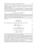
in the figure 1 we have a modular logic controller which consists of three modules and three
synchronized transitions. The initial place of each module has one token. The Petri net
model for a logic controller is a reduced size model, which represents the specifications of
the controller hierarchically. Therefore, the structure and initial marking of a modular logic
controller should be live, safe, and reversible (Murata, 1989).
We notice that the logical behavior of the controller can be ensured from the functional
correctness of its Petri net model. A common and convenient representation of a marked
Petri net is by its state equation.
The main terms involved in the state equation of a Petri net are the incidence matrix, C and
the initial marking M
0
, which can be represented for the modular logic controllers, as the
above given matrix, see relation (10).
Following the definition of an incidence matrix, for a Petri net with k modules and n
i

number of places in the i
th
module, the incidence matrix of each module, C
i
, where i = 1, …,
k, can be represented as a (n
i
x m) matrix, where m is the number of transitions in the
system. This matrix is constructed with the places of each module and the transitions of the
system: C
i
(t).

Fig. 1. An example of a modular logic controller
Module 1
Module 2
Module 3
p
4
p
7
t
2
t
1
p
6
p
3
p
1
p
2
p
5
t
3
Risk and Reliability Analysis of Flexible Construction Robotized Systems

145

7
6
5
4
3
2
1
p
p
p
p
p
p
p
C =
⎥
⎥
⎥
⎥
⎥
⎥
⎥
⎥
⎥
⎦
⎤
⎢
⎢
⎢
⎢

⎢
⎢
⎢
⎢
⎢
⎣
⎡
,
⎥
⎥
⎥
⎥
⎥
⎥
⎥
⎥
⎥
⎦
⎤
⎢
⎢
⎢
⎢
⎢
⎢
⎢
⎢
⎢
⎣
⎡

=
0
1
0
0
1
0
1
M
(10)
The incidence matrix of the system can be constructed using the following equation:
C =
⎥
⎥
⎥
⎥
⎥
⎥
⎥
⎥
⎥
⎥
⎦
⎤
⎢
⎢
⎢
⎢
⎢
⎢

⎢
⎢
⎢
⎢
⎣
⎡
−
−−−
−−−
−
−−−
−
−+
−+
−+
kk
22
11
CC
CC
CC
#
=
⎥
⎥
⎥
⎥
⎥
⎥
⎥

⎥
⎥
⎦
⎤
⎢
⎢
⎢
⎢
⎢
⎢
⎢
⎢
⎢
⎣
⎡
−
−
−
k
2
1
C
C
C
#
(11)
Where
+
i
C and

−
i
C are post and pre – incidence matrices of the i
th
module respectively and
the incidence matrix C is a n x m matrix and c
ij
∈ {0,-1,1}. The initial places of a modular
logic controller are assumed to be the first place of each module and can be represented by
an n-dimensional vector. The initial marking is represented by:

{
}
n
0
0,1 M ∈
(12)

Here 1 represents the initial places of the modules. This modular construction can be easily
modified and reconfigured (i.e. it is suitable for FCRS’s representation) by replacing incidence
matrix of modules. The dynamic evolution of a modular logic controller can be determined
by this incidence matrix and initial marking using the following relation (state equation):

C0
f C M M
⋅
+
=
(13)

Where, f
C
is the firing count vector of the firing sequence of transition f in the net. An
important parameter of the FCRS’s is the resources flow volume. This is determined by the
cycle time of a system in normal operation. Generally, performance analysis of event based
systems is done by adding time specifications to the Petri net model. The performance
analysis of timed Petri nets has been done for the evaluation of the cycle time. For strongly
connected timed marked graphs, a classic method for computing the minimum cycle time
C
T
is given by the following relation (Park 1999), (Tilburg & Khargonekar, 1999):


t
1
t
2
t
3
C
1

⎥
⎦
⎤
⎢
⎣
⎡
−
−

110
110

C
2

⎥
⎥
⎥
⎦
⎤
⎢
⎢
⎢
⎣
⎡
−
−
−
110
011
101

C
3

⎥
⎦
⎤
⎢

⎣
⎡
−
−
011
011

Robotics and Automation in Construction

146

N
(
)
()
⎭
⎬
⎫
⎩
⎨
⎧
=
Γ∈ν
γN
γD
maxC
T
(14)
Where,
Γ is the set of directed circuits of the pure Petri net; D(γ) =

∑
∈γp
i
i
τ
is the sum of times
of the places in the directed circuit
γ; N(γ) is the number of tokens in the places in directed
circuit
γ. As pointed out in (Zhou & Twiss, 1998), the cyclic behavior of timed Petri nets is
closely related to the number of tokens and to the number of states in the directed circuit
which decides the cycle time C
T
. As we know, model analysis and control algorithms
implemented with Petri nets are based on the model state-space, and hence they are
adversely affected by large state-space sizes. Thus, in the next section we’ll give a bottom-up
approach for the state-space size estimation of Petri nets.
5. Size estimation of modular controllers of FCRS’s
In order to estimate the state space of Petri nets, they are divided into typical subnets, i.e.,
subnets with basic interconnections, such as: series, parallel, blocking, resource sharing,
failure repair inter-connection, etc. Each subnet is associated with a state counting function
(Zaitoon, 1996) (SC-function) that describes the subnet’s state-space size when it contains r
“flow” tokens. We notice that “flow” tokens (those that enter and leave the subnet via its
entry and exit paths) are different from control tokens in a controlled Petri net. Petri nets
model the execution of sequential parallel and choice operations, which are abstracted to be
subnets (SN). Figure 2 illustrates two subnets in series, where tokens pass from SN
1
to SN
2
.

The interconnection’s SC-function is given by the following relation (Watson & Desrochers,
1994).

() ()
∑∑
=
−⋅=⋅=
r
0i
21
r
2211series
)ir(S)i(SrSrS (r)S
(15)


Fig. 2. Series interconnection of two Petri subnets
Analogous with the previous approaches, in the figure 3 we have the basic interconnections
for parallel subnets (Fig.3.a); choice among subnets (Fig.3.b); blocking (Fig.3.c), and resource
sharing (Fig.3.d).
The SC-functions (Zaitoon, 1996) for the nets in Fig.3.a, b, c, d are given by relations (16),
(17), (18), (19), respectively:

)r(S (r)S (r)S
21paralel
⋅=
(16)

() ( ) ( )
1irSirSiS (r)S

3
r
1i
21choice
−−⋅−⋅=
∑
=
(17)
SN
1
t
in
t
ou
t
t
SN
2
Risk and Reliability Analysis of Flexible Construction Robotized Systems

147

Fig. 3. Basic interconnections of Petri subnets
In relation (16) places P
in
and P
out
are considered as a group which forms the third subnet.

(

)
wr,
wr,
0
rS
(r)S
1
blocking
>
≤
⎩
⎨
⎧
=
(18)

(
)
(
)
wrr,
wrr,
0
rSrS
(r)S
21
21
2211
share
>+

≤+
⎩
⎨
⎧
⋅
=
(19)

For example, in the figure 4 we have a system composed of three interconnections: the
innermost is a choice between two subnets (each of the places); the middle interconnection is
a resource block with queue; the outermost interconnection is a resource block. The SC-
function for the inner choice is:

2r,
1r,
0r,
10
4
1
=
=
=
⎪
⎩
⎪
⎨
⎧
= S
in(r)
(20)

The SC-function of the middle resource block is:
SN
1

SN
2

t
in
t
out
(a)
SN
1
SN
2
(b)
P
in
P
ou
t
t
in
t
ou
t
t
1
t

2
t
4
t
3
t
in
P
w
t
out
SN
1
(c)

W

t
in2
t
out
t
out1
t
in1
(d)

SN
2
P

w
SN
1

Robotics and Automation in Construction

148

2r,
1r,
0r,
15
5
1
≥
=
=
⎪
⎩
⎪
⎨
⎧
= S
mid(r)
(21)
The SC-function of the outer resource block is:

4r,
4r2,
1r,

0r,
0
15
5
1
S
out(r)
>
≤≤
=
=
⎪
⎪
⎩
⎪
⎪
⎨
⎧
=
(22)


Fig. 4. Example of a multiple interconnection system
Following the above approach for calculating the size of the Petri net models of the modular
controllers, we can adjust or modify the models accordingly to a reasonable size or in order
to achieve the system requirements. We notice that state-space size estimation provides a
tool for the model developer and the resulting data can be used to evaluate detail trade-off.
As noted before, the longest directed circuits of the timed Petri net model determine the
cycle time. Since for a high volume transfer line, the cycle time is determined by a directed
circuit, we can use many of the known results to get more efficient algorithms for finding

the critical operations of a timed modular logic controller (Murata, 1989). For example,
because all transitions in the Petri net model of a modular controller are synchronized, we
can assume that the sequence of transitions for the cyclic behavior is obtained by firing all
transitions in the system only at once. Then the markings of the cyclic behavior of the
system can be generated by the state equation (4) from the initial marking M
0
.
6. The interaction Man-Machine in FCRS’s
A characteristic of high level security control systems, such as those used in FCRS’s is that
an answer to a flaw that makes the man-machine system go to a lower level of security is
considered a false answer, namely a dangerous failure, while an answer leading to a higher
level of security for the man-machine system is considered an erroneous answer, namely a
t
1
P
1
t
2
P
2
t
3
t
7
P
5
t
5
P
3

P
6
t
4
t
6
P
4
P
7
Risk and Reliability Analysis of Flexible Construction Robotized Systems

149
non-dangerous failure. That is the reason for the inclusion of some component parts with
maximum failure probability towards the erroneous answer and parts with minimum
failure probability towards the false answer. One must notice that the imperfect functioning
states of the components of the man-machine system imply the partially correct functioning
state of the FCRS. In the following lines the notion of imperfection will be named imperfect
coverage, and it will be defined as the probability “c” that the system executes the task
successfully when derangements of the system components arise. The imperfect reparation
of a component part implies that this part will never work at the same parameters as before
the derangement (Ciufudean et al., 2008). In other words, for us, the hypothesis that a
component part of the man-machine system is as good as new after the reparation will be
excluded. We will show the impact of the imperfect coverage on the performances of the
man-machine system in railway transport, namely we will demonstrate that the availability
of the system is seriously diminished even if the imperfect coverage’s are a small percent of
the many possible faults of the system. This aspect is generally ignored or even unknown in
current managerial practice. The availability of a system is the probability that the system is
operational when it is solicited. It is calculated as the sum of all the probabilities of the
operational states of the system. In order to calculate the availability of a system, one must

establish the acceptable functioning levels of the system states. The availability is considered
to be acceptable when the production capacity of the system is ensured. Taking into account
the large size of a FCRS, the interactions between the elements of the system and between
the system and the environment, one must simplify the graphic representation. For this
purpose the system is divided into two subsystems: the equipment subsystem and the
human subsystem. The equipment subsystem is divided into several cells. A Markov chain
is built for each cell i, where i=1,2,…n, in order to establish the probability that at least k
i

equipments are operational at the moment t, where k
i
is the least equipment in good
functioning state that can maintain the cell i in an operational state. Thus, the probability of
good functioning will be established by the probability that the human subsystem works
between k
i
operational machines in the cell i and k
i+1
operational machines in the cell (i+1) at
the moment t, where i=1,2,…n; n representing the number of cells in the equipment
subsystem (Thomson & Wittaker, 1996). Assuming that the levels of the subsystems are
statistically independent, the availability of the whole system is:

() ()
tA)t(AtA
h
n
1 = i
i
⋅

⎥
⎥
⎦
⎤
⎢
⎢
⎣
⎡
=
∏
(23)
Where: A (t) = the availability of the FCRS (e.g. the man-machine system); A
i
(t) = the
availability of the cell i of the equipment subsystem at the moment t; A
h
(t) = the availability
of the human subsystem at the moment t; n = the number of cells i in the equipment
subsystem.
6.1 The equipment subsystem
The requirement for a cell i of the equipment subsystem is that the cell including N
i
equipment of the type M
i
ensures the functioning of at least k
i
of the equipment, so that the
system is operational. In order to establish the availability of the system containing
imperfect coverage and deficient reparations, a state of derangement caused either by the
imperfect coverage or by a technical malfunction for each cell, has been introduced. In order

Robotics and Automation in Construction

150
to explain the effect of the imperfect coverage on the system, we consider that the operation
O
1
can be done by using one of the two equipments M
1
and M
2
, as shown in the figure 5.



Fig. 5. A subsystem consisting of one operation and two equipments
If the coverage of the subsystem in the figure 1 is perfect, that is c =1, then the operation O
1

is fulfilled as long as at least one of the equipments is functional. If the coverage is imperfect,
the operation O
1
falls with the probability 1-c if one of the equipments M
1
or M
2
goes out of
order. In other words, if the operation O
1
was programmed on the equipment M
1

which is
out of order, then the system in the figure 1 falls with the probability 1-c (Kask & Dechter,
1999). The Markov chain built for the cell i of the equipment subsystem is given in figure 6.

Fig. 6. The Markov model for the cell i of the equipment subsystem
The coverage factor is denoted as c
m
, the failure rate of the equipment is λ
m
(it is
exponential), the reparation rate is μ
m
(also exponential), and the successful reparation rate
is r
m
, where all the equipments in the cell are of the same type. In the state k
i
the cell i has
only k
i
operational equipments. In the state N
i
the cell works with all the N
i
equipments. The
O
1
M
1
M

2
N
i
FN
i
N
i
-1
FN
i
-1
K
i
+
1
Fk
i
+
1
K
i
Fk
i
N
i
λ
m
(1-c
m
)

r
m
μ
m
(N
i
-1)
λ
m
(1-c
m
)+
μ
m
(1-r
m
)
r
m
μ
m
(K
i
+1)λ
m
(1-c
m
)+μ
m

(1-r
m
)

r
m
μ
m

K
i
λ
m
+
μ
m
(1-r
m
)
r
m
μ
m

N
i
c
m
λ
m

(
N
i
-1
)
c
m
λ
m

(K
i
+2
)
c
m
λ
m

(K
i
+1
)
c
m
λ
m

r
m
μ
m
r
m
μ
m
Risk and Reliability Analysis of Flexible Construction Robotized Systems

151
state of the cell i changes from the work state K
i,
for K
i
≤ k
i
≤ N
i
, to the derangement state
Fk
i
, either because of the imperfect coverage (1-c
m
) or because of a deficient reparation (1-
r
m
). The solution of the Markov chain in the figure 6 is the probability that at least k
i

equipments work in the cell i at the moment t.
The formula of this probability is:

()
∑
=
i
i
i
N
k=k
k
)t(PtA
(24)
Where, A
i
(t)=the availability of the cell i at the moment t; P
ki
(t)=the probability that k
i
operational equipments are in the cell i at the moment t, i=1,2,…,n; N
i
= the total number of
the M
i
type equipments in the cell i; K
i
=the minimum number of operational equipments in
the cell i.

6.2 The human subsystem
The requirement for the human subsystem is the exploitation of the equipment subsystem in
terms of efficiency and security. In order to establish the availability of the operator for
doing his work at the moment t, we build the following Markov chain, which models the
behaviour of the subsystem (Ciufudean et al., 2006):


Fig. 7. The Markov chain corresponding to the human subsystem
Where, λ
h
= the rate of making an incorrect decision by the operator; μ
h
= the rate of making
a correct decision in case of derangement; c
h
= the rate of coverage for the problems caused
N FN
N-1
FN-1

K+
FK+
1
K
FK

N
λ
h
(

1-c
h
)

r
h
μ
h
(N-1)
λ
h
(1-c
h
)+
μ
h
(1-r
h
)

r
h
μ
h
(K+1)λ
h
(1-c
h
)+μ
h

(1-r
h
)

r
h
μ
h

K
λ
h
+
μ
h
(1-r
h
)

r
h
μ
h

N
c
h
λ
h



(
N-1
)
c
h
λ
h

(
K+2
)
c
h
λ
h

(
K+1
)
c
h
λ
h

r
h
μ
h

r
h
μ
h


Robotics and Automation in Construction

152
by incorrect decisions or by the occurrence of some unwanted events; r
h
= the rate of
successfully going back in case of an incorrect decision (Bucholz, 2002).
According to the figure 7, the human operator can be in one of the following states:
The state N = the normal state of work, in which all the N human factors in the system
participate in the decisional process;
The state K = the work state in which k persons participate in the decisional process;
The state F
(k+u)
= the work state that comes after taking an incorrect decision or after an
inappropriate repair that can lead to technological disorders with no severe impact on the
traffic safety, where u=0,…N-k;
The state F
k
=the state of work interdiction due to incorrect decisions with severe impact on
the traffic safety.
In the figure 7, the transition between the states of the subsystem is made by the successive
withdrawal of the decision right of the human factors who made the incorrect decisions.
The working availability of the human factor under normal circumstances is:

()
∑
=
m
j = x
xh
)t(PtA
(25)
Where, P
x
(t) = the probability that at the moment t the operator is in the working state X;
m=the total number of working states allowed in the system; j = the minimal admitted
number of working states.
Assigning new working states to the human factor increases the complexity of the calculus.
Besides, although the man-machine system continues to work, some technological standards
are exceeded, and that leads to a decrease in the reliability of the system.
The highlighting of new states of the human subsystem, that is the development of complex
models with higher and higher precision, renders more difficult because of the increasing
volume of calculus and the decreasing relevance of these models.
In order to lighten the application of complex models of Markov chains, a reduction of these
models is required, until the best ratio precision/relevance is reached.
We notice that it is relatively easy to calculate the probabilities of good functioning for the
machines (engines, electronic and mechanic equipments, building and transport control
circuits, dispatcher installations etc.), while the reliability indicators of the decisional action
of the human operator are difficult to estimate. The human operator is subjected to some
detection psychological tests in which he must perceive and act according to the apparition
of some random signals in the real system man-machine. However, these measurements for
stereotype functions have a low accuracy level.
The man-machine interface plays a great part in the throughput increase of the FCRS’s. The

incorrect conception of the interface for presenting the information and the inadequate
display of the commands may create malfunctions in the system.
7. An example of reliability analysis of construction robotized system
In order to illustrate the above-mentioned method, we shall consider a building site
equipped with electronic and mechanic equipments consisting of three robot arms for
load/unload operations and five conveyors. Two robots (e.g. robot arms) and three
conveyors are necessary for the daily traffic of building materials and for the shunting
Risk and Reliability Analysis of Flexible Construction Robotized Systems

153
activity. That means that the electronic and mechanic equipment for two robots and three
conveyors should be functional, so that the construction materials traffic is fluent.
The technician on duty has to make the technical revision for the five conveyors and for the
three robots, so that at least three conveyors and two robot arms of the building site work
permanently (Ciufudean et al., 2008).
On the other side, the construction engineer has to coordinate the traffic and the
manoeuvres in such a manner as to keep free at least three conveyors and two robot arms,
while the maintenance activities take place on the other two conveyors and one robot.
In this example the subsystem of the human factor consists of the decisional factors: the
designer (i.e. architect), the construction engineer and the equipments technician (electro-
mechanic). The subsystem of the equipments consists of the three robots and five conveyors
(including the necessary devices). This subsystem is divided into two cells, depending on
the necessary devices (e.g. electro-mechanisms and the electronic equipment for the
conveyors, and respectively the electronic and mechanic equipment for the robots).
All the necessary equipments for the conveyors section are grouped together in the cell A
1
,
are denoted by Ap
1…5
and serve for the operation O

1
(the transport of building materials).
The rest of the equipments denoted by E
1…3
are grouped together in the cell A
2
and serve for
the operation O
2
(the load/unload operations of building materials by conveyors),
according to the figure 8.


Fig. 8. The cells structure of the equipment subsystem
In the next table the rates of spoiling/repairing of the components are given.

The components of the system C μ λ r K
i
N
i

A
pi
0.8 1.0 0.03 0.8 3 5
E
i
0.8 0.5 0.025 0.8 2 3
The components of the human
subsystem
0.8 0.2 0.01 0.8 1 1,2,3

Table 1. The failing/repairing rates for the components of the system
A
p1
A
1
A
p2
A
p3
A
p4
A
p5
O
1
A
2
E
1
E
2
E
3
O
2
Robotics and Automation in Construction

154

Fig. 9. The matrix of the state probabilities for the cell A

1
from the equipment subsystem

Fig. 10. The matrix of the state probabilities for the cell A
2
from the equipment subsystem
For the equipment subsystem there are two Markov chains, one with six states (cell A
1
) and
one with four states (cell A
2
); the matrix in the figure 9 corresponds to the first one and the
matrix in the figure 10 corresponds to the second one. The following Markov chains
correspond to the human subsystem:
- with six states (the decisions are made by the three factors: the designer, the
construction engineer and the electro-mechanic);
- with four states (the decisions are made only by two of the above-mentioned factors);
- with two states (the decisions are made by only one human factor).
A matrix of the state probabilities corresponds to each Markov chain:



Fig. 11. The Markov chain corresponding to three of the decisional factors
5
4
3
F
F
F
5

4
3
⎥
⎥
⎥
⎥
⎥
⎥
⎥
⎥
⎥
⎦
⎤
⎢
⎢
⎢
⎢
⎢
⎢
⎢
⎢
⎢
⎣
⎡
λ−μ
λ−μ
λ−μ
λλ−λ
μ+λμμ+λ−λ
μ+λμμ+λ−

)8,0(008,000
0)8,0(008,00
00)8,0(008,0
00)5(40
02,08,008,0)4(
2,3
002,0308,03
FFF543
543

⎥
⎥
⎥
⎥
⎥
⎦
⎤
⎢
⎢
⎢
⎢
⎢
⎣
⎡
μ−μ
μ−μ
λ
λ
−λ
μ

+
λ
μμ+λ
−
)
8,0
(08
,
00
)8
,0
(0
8,
0
6
,
00)
3
(4
,
2
02
,
02
8,
0
)2
(
F
F

3
2
3
2
2 3 F
2
F
3
3
2
1
F
3

F
2

F
1

3
λ
h
(1-c
h
)

r
h
μ

h
2λ
h
(1-c
h
)+μ
h
(1-r
h
)
λ
h
+μ
h
(1-r
h
)
r
h
μ
h

r
h
μ
h

r
h
μ

h
r
h
μ
h
3c
h
λ
h
2c
h
λ
h

Risk and Reliability Analysis of Flexible Construction Robotized Systems

155

Fig. 12. The matrix of the state probabilities corresponding to the Markov chain in the Fig.11

Fig. 13. The Markov chain corresponding to two decisional factors
⎥
⎥
⎥
⎥
⎥
⎥
⎦
⎤
⎢

⎢
⎢
⎢
⎢
⎢
⎣
⎡
μ−μ
μ−μ
λλ−λ
μ+λμμ+λ−
)8,0(08,00
0)8,0(08,0
4,00)2(6,1
02,08,0)(
FF21
F
F
2
1
21
2
1

Fig. 14. The matrix of the state probabilities corresponding to the Markov chain in the Fig.13

Fig. 15. The Markov chain corresponding to one decisional factor

Fig. 16. The matrix of the state probabilities corresponding to the Markov chain in the Fig.15
The equations given by the matrix of the state probabilities are functions of time and by

solving them we obtain:
3
1
F
F
F
3
2
1
⎥
⎥
⎥
⎥
⎥
⎥
⎥
⎥
⎥
⎦
⎤
⎢
⎢
⎢
⎢
⎢
⎢
⎢
⎢
⎢
⎣

⎡
μ−
μ−μ
μ−μ
λλ−λ
μ+λμμ+λ−λ
μ+λμμ+λ−
)8,0(008,000
0)8,0(008,00
00)8,0(008,0
6,000)3(4,20
02,04,008,
0)2(6,1
00208,0)(
FFF321
321

2
F
2

1
F
1
2
λ
h
(1-c
h
)

2c
h
λ
h
r
h
μ
h
λ
h
+
μ
h
(1-c
h
)
r
h
μ
h
1
F
1
r
h
μ
h

λ
h

+
μ
h
(1-r
h
)
1
F
1
⎥
⎥
⎥
⎦
⎤
⎢
⎢
⎢
⎣
⎡
μ−μ
μ+λμ+λ−
)8,0(8,0
2,0)2,0(
F1
1

Robotics and Automation in Construction

156
- The expressions of the availabilities for the cell A

1
, and respectively A
2
from the
equipment subsystem calculated with the relation (18);
- The expression of the availability of the human subsystem calculated with the relation
(19);
- The expression of the availability of the whole system calculated with the relation (17).
The values of these availabilities depending on time are given in the table 2.

Time
[hours]
Cell
A
1

Cell
A
2

The human
subsystem
A
h

The availability of the
railway system
A
0 1.000000 1.000000 1.0000000 1.00000000
1 0.980013 0.985010 0.9548293 0.92171802

4 0.947011 0.951341 0.8645392 0.77888946
8 0.933510 0.933468 0.8061449 0.70247605
12 0.933010 0.927481 0.7809707 0.67581225
16 0.933129 0.926133 0.7701171 0.66553631
20 0.933060 0.925951 0.7654364 0.66131243
24 0.932891 0.925600 0.7647893 0.65970171
28 0,932762 0,925012 0,7635876 0.65876005
32 0.932132 0.924910 0.7631243 0.65781145
36 0.931902 0.924830 0.7625786 0.65716133
40 0.931819 0.924690 0.7621289 0.65640272
44 0.931791 0.924600 0.7619786 0.65640272
48 0.931499 0.924582 0.7619456 0.65618425
Table 2. The availability values for the elements of the exemplified system
8. Conclusion
An advantage of the above-mentioned calculus method is the easy calculation of the
availability of the whole system and of the elements of the system. The availabilities of the
exemplified system are drawn in figure 17, depending on time and on the number of
decision factors. In figure 17, the numbers x=1,2,3 show the availability of the systems
corresponding to the Markov chains in figure 11, figure 13, respectively figure 15. The figure
17 shows that the best functioning of the system can be obtained by using two decisional
factors: while the availability of the system in figure 15 is 65% after 12 hours of functioning,
the availability of the system in figure 13 is 82%. The availability of the system decreases
when the third decisional factor appears, because the diminution due to the risk of imperfect
coverage or due to an incorrect decision is greater than the increase due to the excess of
information.
In the figure 18 the availability of the system depending on the coverage factors (c
m
), and on
the successful repairing (r
m

) of deficient equipment is illustrated. One may notice that the
availability increases with 5 percents when the coverage is perfect (c
m
=1). Moreover, when
the repairing of a deficient equipment is perfect (r
m
=1), the availability increases with 10
percents (we mention that the increases refer to a concrete case where c
m
=0.8 and r
m
=0.8).
An important conclusion that we can draw is that the presumption of perfect coverage and
repairing affects the accuracy of the final result. This presumption is made in the literature
in the majority of the analysis models of the system availability (Hopkins, 2002).
Risk and Reliability Analysis of Flexible Construction Robotized Systems

157

Fig. 17. The availability of the railway system depending on the number of the decisional
factors

Fig. 18. The variation of the system availability depending on the factors c
m
and r
m

The analysis of the availabilities of the operation O
1
and O

2
done by the cell A
1
and
respectively by the cell A
2
from the equipment subsystem shows that an increase of the
number of the conveyors (from N
i
=5 and k
i
=3 to N
i
=5 and k
i
=4) in the cell A
1
would lead to
a decrease of the availability of the operator O
1
with 4% (as shown in the figure 19). In the
case of the cell A
2
, a decrease of the total number of robots (from N
i
=3, k
i
=2 to N
i
=2, k

i
=2)
would lead to a decrease of the availability of the operator O
2
with 20% (as shown in the
figure 20). The conclusion is that an extra robot is critical for the system, because it improves
considerably the availability of O
2
and hence, the availability of the system.


Fig. 19. The analysis of the availability of the cell A
1
The analysis of the availability allows us to establish the lapse of time when changes must
be made in the structure of the system (major overhaul, the rotation of the personnel in
shifts etc). For example, from the figure 17, if the availability is 70%, the human decisional
factor must be replaced every 12 hours (for the system in the figure 15 that is rotating the
personnel every 12 hours).
Robotics and Automation in Construction

158

Fig. 20. The analysis of the availability of the cell A
2

9. References
Aven, T. (2004). Risk Analysis and Science, International Journal of Reliability, Quality and
Safety Engineering, vol. 11, no. 1, pp. 1-15
Ferrarini, L. (1992). An incremental approach to logic controller design with Petri nets, IEEE
Trans. Syst. Man. Cybern., vol. 22, pp. 461-473

Ferrarini, (1994). L. A new approach to modular liveness analysis conceived for large logic
controllers design, IEEE Trans. Robot. Automat, vol. 10, pp.169-184
Zaitoon, J. (1996). Specification and design of logic controllers for automated
manufacturing systems, Robot. Comput-Integr. Man., vol. 12, no. 4, pp. 353-366
Murata, T. (1989). Petri nets: Properties, analysis and applications, Proc. IEEE, pp. 541-580,
Zhon, M. C. & DiCesare, F. (1992). Design and implementation of a Petri net based supervisor for
a flexible manufacturing system, IFAC J. Automatica, vol. 28, no. 6, pp. 1199-1208
Park, E.; Tilburg D.; Khargonekar, P. (1999). Modular logic controllers for machining
systems: formal representation and performance analysis using Petri nets, IEEE
Trans. Rob. and Autom., vol. 15, no. 6, pp. 1046-1060
Watson J. & Desrochers, A. (1994). State space size estimation of Petri nets: a bottom-up
perspective, IEEE Trans. Rob. and Autom., vol. 10, no. 4, pp. 555-561
Zhou M. & Twiss, E. (1998). Design of industrial automated systems via relay ladder logic
programming and Petri nets, IEEE Trans. Man. Cyber,vol.28,pp.137-150
a. Hopkins, M. (2002). Strategies for determining causes of events, Technical Report R-306,
UCLA Cognitive Systems Laboratory
b. Hopkins, M. (2002). A proof of the conjuctive cause conjecture in causes and explanations,
Technical Report R-306, UCLA Cognitive Systems Laboratory
Thomson, M. G. & Wittaker, J. A. (1996). Rare Failure State in a Markov Chain Model for
Software Reliability, IEEE Trans. Reliab. 48(2), pp. 107-115
Kask, K. & Dechter, R. (1999). Stochastic local search for Bayesian networks, In Workshop on
AI and Statistics 99, pp. 113-122
Russell, S. & Norvig, P. ( 2003). Artificial Intelligence: A Modern Approach, J. Willey and Sons, N.Y.
Bucholz, P. (2002). Complexity of memory-efficient Kroneker operations with applications
to the solutions of the Markov models, Informs J. Comp., no. 12(3), pp. 203-222
Ciufudean, C. & Graur, A. & Filote, C. (2006). Determining the Performances of Cellular
Manufacturing Systems, In Scientific and Technical Aerospace Reports, vol.14, Issue 6,
NASA, Langley Research Center, USA
Ciufudean, C. & Filote, C. & Amarandei, D. (2008). Scheduling Availability of Discrete Event
Systems, The 14th IEEE Mediterranean Electrotechnical Conference, MELECON’2008,

Palais des Congrès François Lanzi - Ajaccio – France.
10
Precast Storage and Transportation Planning
via Component Zoning Optimization
Kuo-Chuan Shih, Shu-Shun Liu and Chun-Nen Huang
National Yunlin University of Science and Technology
Kainan University
Taiwan (ROC)
1. Introduction
Industry management issues, such as enterprise resource planning (ERP) and supply chain
management (SCM), are discussed and implemented successfully in many manufacturing
industries but construction. No matter what the nature of construction is manufacturing
buildings, risks and uncertainties make its characteristic different to other manufacturing
industries. In order to reduce effects of these two scourges, precast is an evolutional method
what is adopted to remove construction work environment from outdoor to indoor and
make the procedure of component producing regular as an automatic factory. Thus, precast
method is a construction method with its industrial characteristics being closest to those of
manufacture industry. However, Practical plans and information identification in working
process must be further recognized and achieved. This study proposes an optimization
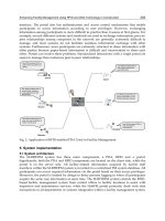
model which focuses on planning issues of precast manufacturing procedure.
The storage and transportation planning of a construction precast project is mainly
discussed herein. Generally, whole process of a precast project can be divided into 5 stages:
design, production, storage, transportation, and installation. Besides, at least 4 important
roles: client, architect, subcontractor, and precast factory, are involved in these 5 stages.
Relationships among these four roles depend on contracts of a project. From perspective of
the precast factory, two stages are out of their control: design stage and installation stage. In
design stage, the architect confirms details of all precast components, such as shape,
strength and material, with the client, and then makes components exact. The precast
factory receives these component details and then produces components according to
architect’s designs as orders. In installation stage, the subcontractor installs all completed

components at where the places according to architect’s design. The precast factory supplies
components on time in the installation stage of most cases. It is obvious that the design stage
and the installation stage involves two or more roles. Thus, production, storage, and
transportation stage are more controllable than these two stages from precast factory’s
viewpoint. Furthermore, production stage was the issues most frequently investigated and
analyzed in prior precast management related study. However, the planning of storage and
transportation are still very significant to a precast factory. To complete the management
mechanism of precast factory, these two stages need to be investigated.
Robotics and Automation in Construction

160
2. Reference
There are many production stage related studies of precast related studies can be referred
and enumerated. For example, Chan has studied a lot in precast production planning. In
order to suit different standardization degrees of components, Chan (2002) has proposed
two production planning models are comprehensive method, which the method utilizes
resources regularly in component producing, and specialized method, which the method
considers low standardization components, for factory business organization. Furthermore,
a coordinated production scheduling and rescheduling model has proposed by Chan (2003,
2005) to deal with risks of component demand. Chan (2005) has adopted simulation to build
scenarios of viaduct producing for analysis. Considering resource-constrained environment,
Leu (2002) has proposed a GA base scheduling model that discussed the importance of
manpower, cranes, steam curing capacity and reinforcement cage storage space. Besides,
Viaduct precast considers both supply-demand matching and high productivity.
Storage and transportation planning issues of precast project have been few studied in
construction field but manufacturing industry. Storage and transportation plan are two
sides of a coin that are presented in many studies in manufacturing industry field. A
common study type is the total cost optimization of transportation among factory,
warehouse and customer. Furthermore, outsourcing of inventory and transportation may be
related to time-base and quantity-base issues (Sıla, 2006). For precast project, how to store a

special object such as precast component which reduce secondary movement and
component finding is a key question. The Acheson & Glover Group (2006) tried to develop a
precast storage system. However, ways to store component are also related to safety of
labor. For construction process issues in job-site, Hu (2005) proposed a geometric reasoning
method that can help to determine the component sequence of demand. Nevertheless,
characteristics of construction precast component: huge; heavy; unique in design or
installation procedure cause these achievements cannot easily perform in precast factory.
One of problem of precast storage and transportation is huge component. However,
containerization is an issue that is valuable to be explored. Vis and Koster (2002) discussed
the process of transporting containers from ship to stack in terminal. Means are used to
move huge objects, including cranes, vehicles, straddle carrier… etc. Thus, a plan to simplify
the process and to use these means efficiently is necessary. Avriel (1998) proposed a
mathematic model that tried to deal with the storage planning problem and reduce the
shifts of container in a ship. However, the size of the precast component is not the only item
to be concerned of one should also be concerned about the different shapes of the
component. Sadiq (1996) proposed a cluster-analysis base model the classified all the objects
into several sets, then allocated all the sets to different storage zones. This model tried to
link the relationship between objects to reduce secondary-movement for objects. The cluster-
analysis can also work in precast project and a cluster-analysis named zoning strategy in
precast project will be discussed herein.
3. Precast component storage and transportation
Optimization is a usual tool for precast factory planning in previous production stage’s
researches. Thus, this research follows mathematical model discussion with more concern in
storage and transportation stages.
Precast Storage and Transportation Planning via Component Zoning Optimization

161
3.1 Storage stage
Generally speaking, storage stage had been considered in the component producing
planning but simplified as an inventory calculation. Daily inventory is a vehicle variable

between component producing and the demand. Produced components are stored in factory
as inventory and this inventory add up all produced components in factory in a period. In
order to match the demand, the component inventory must equal to or exceed the demand
of contract at the deadline of project. Thus, a component producing plan considers daily
inventory is able to create, and it is still practical for factory business mainly considering
production stage. Furthermore, the cost of inventory can be also calculated through the
quantity of stored components, and the inventory limits can be restrained if storage space is
further concerned as constraints. Nevertheless, traditional precast factory can perform this
kind of production planning formulation without considering how to store components.
Component storage must be planed from perspective of a precast factory business. No
matter how a precast factory closed to a manufacturing one, the nature of product of precast
factory, construction component, is very unique to other industries. In addition, there are
less consistent among components when component’s sharp, strength and position of a
building are in consideration. A component that is unique to any other one is commonly
concerned in most construction precast project. Thus, to identify each component is usually
important in storage stage. Furthermore, there are several circumstances must be regarded
in practical storage work: size of components; limitation in vertical loading of ground; safe
distance between components and ways to store components. Briefly, the problem of
component storage is a 2-dimensional or 3-dimensional spatial allocation with component
identification. These considerations cause component storage complex and identification of
component is necessary. It is hard to ignore the storage stage to a precast factory business.
A good storage plan is also benefit to help component delivering in right order and on time.
Two sequences are accompanied with component delivering are sequence from production
stage to storage stage and sequence from storage stage to installation stage. In the first case,
components and molds can be grouped that had mentioned by Chen 2005. In order to
produce components smoothly and continually, Components which can be grouped into a
same sharp, strength and material can be produced orderly by the same mold or grouped
molds which belong to the same category certainly. Under this circumstance, components
can be produced as soon as possible in production stage with minimal operation change of
mold. This sequence is named production sequence, PS, in this research that means

components are delivered according to their group. Besides, PS always causes grouped
components storage. The other sequence is named installation sequence or IS. Components
must be installed at the positions where they are appointed in architect’s design. Thus,
components which belong to the same scope of once installation work, for example a one-
floor installation, are needed in a short moment. Therefore, components are delivered
according to their demand timing from factory to installation worksite. By view of these two
sequences, it can be recognize that there is a conflict between PS and IS in precast factory
business. Therefore, the functionality of storage plan is not only a quantity calculation of
component inventory, but rearrangement of component sequence from PS to IS to resolve
this conflict before their installation.
Foreign site storage that component are stored in a space out of both factory and work site is
another issue in practical factory business. When the space of the precast factory is
insufficient to store all components, foreign site storage is a common alternative. Extra
movements of components are needed to deliver components between different sites.
Robotics and Automation in Construction

162
Foreign site storage refers that the precast factory has to look for other storage sites to store
the components that cannot be stored in the precast factory during project period. This
Foreign site storage issue combines component storage and transportation, and it is complex
in both storage and transportation planning. This alternative occurs in practice. Therefore,
further component planning and controlling mechanism in storage stage is needed to
analysis all above issues for a precast factory.
3.2 Transportation stage
Transportation stage is ignored in previous precast management researches. Components
always produced with few redundancies in a construction precast project, and all of them
must be transported for installation to meet project requirement. Therefore, the cost of
transportation can be treated as a fixed cost in most cases without detail delivery
consideration because component delivery is necessary in a project. Thus, component
transportation has been a parameter of fix cost which does not need to plan. However, the

component transportation still plays an important role in factory business.
There are two kinds of transportation must be recognized in factory business: component
movement within a site and component transportation between two sites for a long
distance. Component movement within a site means that components are moved within the
factory, a storage site, or the work site in short distance. Equipments such as cranes and
trams can be utilized for this case. These equipments are owned or rented for daily business
by precast factory. Hence, transportation cost in this case can be neglected from single
precast project or transformed onto the cost for factory or site setting cost. The other,
component transportation for a long distance is performed by trucks. In practice, trucks are
mostly rented case by case when components transport in sites or turn over from any site to
work site are sure. Two important factors: weight of components and transported distance
are commonly adopted for truck rental fee calculation. This long distance transportation is
variable case by case. For example, components are delivered from the factory to a foreign
site, the factory to the work site, and a foreign site to the work site.
4. Component zoning strategy
Taking to above issues as well as problems with component storage and transportation into
consideration, a mechanism for precast factory planning which employed the concept of
basic zoning with minimization of total cost is purposed. The related definitions and
assumptions are explained in the following sections:
4.1 Component Zoning
Components are grouped into zones herein. A zone is a space that components can be
stored following specific rules which assigned by planner. This component zoning is most
like the behavior of the goods package in manufacturing that goods can be encased into a
box by fallowing rules of what kind of box it is. By the way, a box is both storage and
transportation strategy basis. However, there is no real box for precast component, but it can
be instead by a specified storage space as a zone without encasement. A zone is also similar
to a container to collect components. Components can be moved in respectively. Therefore,
the behavior of a zone is flexible that dependent on rules what the planner made to form it
as a box or container. However, the rules of zones must be clearly declared before planning.
Precast Storage and Transportation Planning via Component Zoning Optimization

163
Zones are able to be alternated to release storage space too. This study mainly focus on how
zoning strategy working in storage and transportation stage to represent component zoning.
To recognize zoning rules is benefit for precast factory planning and management issue.
Zones try to retain the flexibility of storage that planner can declare their own rule. Whole
storage and transportation process can be formed by zones and their own rules. Zoning
rules of a zone basically contain what kind of component can be stored, how many
components can be stored, how much space are required and other specific rules what made
by planner. Zoning rules help planner to control storage and transportation process because
zones can force components well-regulated in preset rules. Thus, making zoning rules
appropriate is a further important issue to meet the request of factory business
management. The PS, to store grouped component, and IS, to store component by
installation scope, are mainly discussed in component zoning herein.
The component zoning according to grouped component occurs in PS that is the common
situation in practical storage business. To store components by group has several
advantages: Components can be easily found; the space utility is well in most of cases;
storage space demand can be easily calculated. This is why most factories which include all
kinds of industry store goods by group of goods type for warehousing, and most of precast
factories are working without exception. However, this kind of zoning strategy is not
always suit precast factory storage. Hundred or thousand of component groups always
occur because of architect’s design.


Fig. 1. Zones by following PS
Figure 1 shows a possible case of PS zoning rules and normal storage practice. Components
are grouped and stored into zones in storage stage. However component searching or
component rearrangement are needed before component installation because IS occurs after
transportation stage. Trucks must find out required components through overall zones for
component searching, or operations in work site must rearrange components before

installation. Additional time and cost are caused in practical. Nevertheless, it can be also a
choice in consideration.
Zoning with IS aim to overcome the conflict between PS and IS in factory. Component
movement within a site is easier and cheaper than long distance transportation of trucks
because cranes and trams can move and rearrange components conveniently. Thus, only
component rearrangement is needed in storage stage. Figure 2 shows this situation.
Robotics and Automation in Construction

164

Fig. 2. Zones by following IS
4.2 Zoning strategy
A zoning strategy is composed by zones what are chose for a storage and transportation
plan during a planned period. Thus, a zoning strategy can contain zones with same rules,
zones with different rules, mutualism zones, and mutually exclusive zones if they are
needed. All zones whether PS or IS are alternatives when planner do not really recognize
what kind of zone rules are suitable before practice. Planner can create kinds of zones and
manifold rules in zones if they are recognized before or during decision making procedure.
An optimization model for seek out the optimal zoning strategy with minimal operation
cost of precast factory in storage stage and transportation stage by zone selection and
allocation is proposed as below.
4.3 Zone selection and allocation
From perspective of component storage, zones are used as basis elements for checking the
component storage and utility of each storage site. In order to form an optimized zoning
strategy, procedure of picking up appropriate zones, in term of zone selection, is very
important. Figure 3 shows a possible situation of zone selection. First at all, components
must be collected into zones fallowing the rules of each zone is a basic assumption. This
assumption makes sure that whole process of component storage can be represented by
zones. Beside, whole inventory space is divided into sites. Two kinds of site that are site
inside factory and foreign site are involved according foreign site inventory behaviour, extra

site rental fee are considered if a foreign site is adopted during the period of a project. This
rental fee contains land usage fee and necessary facility fee to operate storage business.
Besides, truck rental fee can also be recognized by location of a foreign site and weight of
component which are planned to store in this site.
The zone selection can be explained as relationships among components and zones.
Components must be stored for sure, so that at least one zone must exist whenever any
components are stored in. In other word, this zone is adopted when any component is
planed to be stored in. For example, zone 1, 2, 3, and 5 in figure 3 are selected to store
components. On the contrary, zone 4 is not selected to store any component. Besides,
component can be stored into a zone when only they are permitted by rules of this zone.
Precast Storage and Transportation Planning via Component Zoning Optimization

165

Fig. 3. Illustration of the Relationship among Zones and Storage Sites
The zone allocation can also be present as relationship among zones and sites. As the same
circumstance, at least one site must be used or rented because there is at least one zone must
be adopted to store components. A zone can be allocated into a site, no matter site inside
factory or foreign site, when the storage space of this site is sufficient. The required storage
space of this zone is according as its zone rules. Site inside factory or foreign site is allowed
to allocate zones, but one zone can be only allocated once and into one site during a planed
period. Figure 3 shows that site 1 and site 2 inside factory are occupied by zone1, zone 2 and
zone5, and foreign site 1 is occupied by zone 3 respectively. It is allowed that two or more
zones allocated in a site. Besides, whenever a foreign site is selected, the rental fee that
contains land usage fee and the charge of necessary resource to operate storage business will
be added into project cost for entire project period.
4.4 Transportation between sites
The whole transportation problem can be divided into 3 layers component movement
according to zone allocation that mention above are: 1. Factory, in other word production
stage, to sites inside factory; 2. sites inside factory to foreign site; 3. sites to work site, in

other word installation stage. The route of component transportation diagram is shown in
figure 4 as follows:


Fig. 4. Component transportation layer
Robotics and Automation in Construction

166
Two types of transportation, within a site and long distance transportation, can be identified
into these 3 movements. The case of transportation within the same site occurs when
components are moved from factory to sites inside factory, layer 1, obviously. No extra
transportation cost will be charged because these movements are completed by equipments
belonging to factory. The other, long distance movement occurs in layer 2 and 3 and the
truck rental fee according to weight of components and distance between sites will be
charged.
5. Storage-transportation optimization model
5.1 Cost classification of model
Base on the proposed component zoning method, the whole procedure of component
storage and transportation can be integrated and transferred into a problem of zone
selection and allocation. A mathematic optimization model that belong to mix-integer
planning, MIP, has been developed. The objective function of this model is to minimize total
cost in whole storage and transportation stage of precast factory. Inventory cost has been
further divided into two parts, inside and outside factory, that presented as function (2) are
site fee of selected sites. In addition, the transportation cost has been divided into at least
three parts that presented as function (3) according to different truck rental fee calculation.
The structure and classification show as fig 5.


Fig. 5. Cost Classification Chart of the Model
Objective function Minimize

TCICCostTotal
+
=
_ (1)
Where IC is the sum cost in storage stage and TC is the sum cost in transportation stage.

∑∑
+=
np
i
ni
j
jjii
icsUIpcsUPIC ** (2)
Precast Storage and Transportation Planning via Component Zoning Optimization

167
Where i is the index of each site inside factory; np is the total number of sites inside factory;
i
UP are binary variables for judgment of usage for each site i by 0 or 1;
i
pcs are parameters
of site maintain or holding cost of each site when UP
i
are value 1; j is the index of each
foreign site; ni is the total number of foreign site; UI
j
are binary variables for judgment of
site usage for each site j by 0 or 1; ics
j

are parameters of site rental and holding cost of each
site when UI
j
are value 1.
pcs
i
and ics
j
are fixed in consideration of single precast project. Besides, foreign site must be
rented until project is completed.

∑∑∑∑ ∑∑∑∑
−++=
ns
k
ns
l
ct
m
p
n
ns
k
ns
l
ct
m
p
n
mnmlknmmmnmlk

tcTSQdtctcTSQTC 3*)()21(*
,,,,,,,
(3)

Where k and l are both the index of zone. These two parameters present the index of zone
that components are transported from and components are transported to respectively
when transportation between zones occurs. These situations occur in transportation
between sites from inside factory to foreign site; ns is the total number of zones; m is the
index of component type considering its sharp, weight and strength; ct is the total number
of component type; n is the index of project time by working days; p is total working days of
whole project period; TSQ
k,l,m,n
are positive variables to calculate the quantity of component
transportation between zones; tc1
m
are parameters of component transportation cost
between zones which are calculated by distance and weight of component; tc2
m
are the
parameters of component transportation cost from foreign site to worksite which are
calculated by distance and weight of component; d
m,n
are parameter of component demand
of worksite which present component type and working day as a two dimension matrix;
tc3
m
are the parameters of component transportation cost from sites inside factory to
worksite which calculation by distance and weight of component.
The demand of components is fixed after design stage of a project. In addition, there are 2
paths the components can be only transported by zones inside factory to worksite through

foreign site or zone inside factory to worksite directly. The component demand, parameter
d
m,n
, of worksite is equal to sum of the component number which transported through these
2 paths and also equal to total sum of produced component of a project in main
consideration. Beside, foreign site are rented till the end of project and cannot retain
component. Thus, the quantity of transported component from site inside factory to foreign
site is equal to the quantity of transported component from foreign site to worksite.
Constraints:
Function (4) - (8) present rules of zone selection and allocation in whole project period.
Judging of site usage

∑∑
≥∀
ns
k
p
n
niki
SLPUPMi
,,
*
(4)

∑∑
≥∀
ns
k
p
n

njkj
SLIUIMj
,,
* (5)