Supply Chain, The Way to Flat Organisation Part 4 pdf

Optimization Based e-Sourcing

81
- Supply Constraint: For every winning bid Jj
′
∈ , ],[
jjj
zaq
∈
, and for losing bids, .0=
j
q
-
Demand Constraint: The total quantity procured should satisfy the demand of the buyer:
.Bq
Jj
j
≥
∑
′
∈

The WDP is a nonconvex piecewise linear knapsack problem (Kameshwaran & Narahari,
2009a), which is
NP-hard. It is a minimization version of a nonlinear knapsack problem with
a demand of
B
units. Each bid corresponds to an item in the knapsack. Unlike traditional
knapsack problems, each item
j can be included in the knapsack in a pre-specified range
],[

jj
za and the cost
j
Q is a function of quantity included.
The cost function
j
Q of Figure 3 is nonlinear but due to the piecewise linear nature, the
WDP can be modelled as the following MILP.

()
∑∑
∈=
⎟
⎟
⎠
⎞
⎜
⎜
⎝
⎛
++
Jj
l
s
s
j
s
j
s
j

s
j
s
jjj
j
xdndn
1
00
min
δβ
(1)
subject to

01
jj
dd ≤ Jj ∈∀ (2)

s
j
s
j
dx ≤
j
lsJj
≤
≤
∈
∀
1 ; (3)

1+
≥
s
j
s
j
dx
j
lsJj
<
≤
∈
∀
1 ; (4)

Bxda
Jj
l
s
s
j
s
jjj
j
≥
⎟
⎟
⎠
⎞
⎜

⎜
⎝
⎛
+
∑∑
∈=1
0
δ
(5)

{
}
1,0∈
s
j
d

j
lsJj
≤
≤
∈
∀
0 ; (6)

[
]
1,0∈
s
j

x
j
lsJj
≤
≤
∈
∀
1 ; (7)
The decision variable
s
j
x denotes the fraction of goods chosen from the linear segment
s
of
bid
.j For this setup to make sense, whenever 0>
s
j
x then
,0
1
=
−s
j
x
for all
.s
To enable this,
binary decision variable
s

j
d
is used for each segment to denote the selection or rejection of
segment
s
of bid .j The winning quantity for bid j is
∑
=
+
j
l
s
s
j
s
jjj
xda
1
0
δ
with cost
()
∑
=
++
j
l
s
s
j

s
j
s
j
s
j
s
jjj
xdndn
1
00
δβ
. The binary decision variable
0
j
d is also used as an indicator
variable for selecting or rejecting bid
,j
as 0
0
=
j
d implies that no quantity is selected for
trading from bid
.j

3.4 Business constraints
The business rules and purchasing logic can be added as side constraints to the WDP. For
the above procurement scenario, the relevant business constraints are restricting the number
of winning suppliers in a given range [

LB, UB] and guaranteeing a minimum volume (or
monetary business worth)
MIN_QTY (MIN_VAL) for a set of incumbent suppliers JJ ⊂
'
.
Supply Chain, The Way to Flat Organisation

82
UBdLB
Jj
j
≤≤
∑
∈
0
(8)

QTYMINxda
Jj
l
s
s
j
s
jjj
j
_
'1
0
≥

⎟
⎟
⎠
⎞
⎜
⎜
⎝
⎛
+
∑∑
∈=
δ
(9)

()
VALMINxdndn
Jj
l
s
s
j
s
j
s
j
s
j
s
jjj
j

_
'1
00
≥
⎟
⎟
⎠
⎞
⎜
⎜
⎝
⎛
++
∑∑
∈=
δβ
(10)
The above constraints can be added as side constraints to the WDP. Usually one of the (9) or
(10) is used. Business rule that limits the winning quantity or business value for a winning
supplier can be implicitly included by suitably modifying the supply range ],[
jj
za .
3.5 Algorithms
Dynamic programmic based exact and approximation algorithms were proposed in
(Kameshwaran & Narahari, 2009a) and a Benders’ decomposition based exact algorithm was
proposed in (Kameshwaran & Narahari, 2009b) to solve the WDP formulated as (1)-(7).
Similar procurement scenarios have been considered in the literature with various
assumptions. Kothari et al. (2003) expressed the cost function using fixed unit prices over
intervals of quantities (piecewise linear but continuous with no jump costs) and
approximation algorithms based on dynamic programming were developed for solving the

WDP. Procurement with nonconvex piecewise linear cost functions was considered by
Kameshwaran & Narahari (2005) with the additional business constraint of restricting the
number of winning suppliers. A Lagrangian based heuristic was proposed to solve the
WDP. Eso et al. (2005) considered the quantity discount procurement of heterogeneous
goods and column-generation based heuristic was proposed to solve the WDP.
3.6 Other discount based sourcing techniques
In the above, we briefly discussed about volume discounts offered while procuring multiple
units of a single item. Eso et al. (2005) considered buying multiple items with volume
discounts for each item. There are two kinds of discounts for procuring multiple units of
multiple items:
Business volume discounts (Sadrain & Yoon ,1994) and total quantity discounts
(Goossens et al. 2007). In the business volume discounts, the discounts are based on the total
monetary worth of the purchase rather than on the quantity. This discount structure is
applicable in telecommunication sourcing. In total quantity discounts, discount is based on
the total quantity of all items purchased. This discount is used in chemical and also in
telecom capacity sourcing. Exact algorithms based on brand and bound were proposed in
(Goossens et al., 2007) to solve this problem. For a special case with single unit demand for
multiple items, a suite of branch-and-cut algorithms was proposed in (Kameshwaran et al.,
2007).
4. Combinatorial sourcing
Consider a sourcing scenario where the buyer wants to buy a set of heterogeneous items.
Two immediate approaches to procure them are in
sequence (sequential procurement with
one after another) and in
parallel (all items are procured simultaneously by conducting a
Optimization Based e-Sourcing

83
sourcing auction for each item separately). The third option is to conduct a combinatorial
auction

where the supplier can bid on a combination of items by providing a single bid price
(Cramton, 2006). Thus the bid price is conditional on winning the entire combination of
items. These auctions are ideal for scenarios in which synergies exist between the items.
Suppose a supplier obtains more profit by selling a set of items together, then he can submit
this
all-or-nothing combinatorial bid by providing a discounted price on that entire package.
The supplier can submit more than one bid and the items in different bids can be
overlapping.
Combinatorial auctions were initially used in selling scenarios like airport slot allocation
(Rassenti et al., 1982) and radio spectrum auctions (Rothkopf et al., 1998). The sourcing
applications mainly include procurement of transportation services (Caplice & Sheffi, 2006),
in addition to direct sourcing of industrial inputs (Hohner et al., 2003). In this following, we
present various combinatorial bids and the respective WDP formulations.
4.1 Static package bids
Let the items to be procured be indexed by i, each with demand d
i
. A bidder j bids on a
package or bundle of items, providing a single bid price for that bundle. Let the package be
indexed by
k. As mentioned above, the bidder can submit different packages as bids with
possibly overlapping items. The winner determination problem can be formulated as the
following 0-1 integer program.

min
kk
jj
jk
Cy
∑
∑

(11)
subject to

:
kk
ij j i
jkik
yd
δ
∈
=
∑
∑
i
∀
(12)

{
}
0,1
k
j
y ∈ kj,∀ (13)
where the notations are:
Indices
i
Item identification
j

Supplier identification

k
Package identification
Decision variables
k
j
y
= 1 if supplier
j is assigned package k = 0, otherwise
Data
k
j
C
Bid price for package k of supplier j
k
ij
δ

Volume of item
i as a part of package k for supplier j
The objective function (11) minimizes the total procurement cost. The constraint (12)
enforces the demand requirements of the buyer. The above formulation allows for each
supplier to win more than one package bids. This is
OR bidding language (implying logical
OR). Another popular bidding language used in practice is
XOR, which allows at most one
Supply Chain, The Way to Flat Organisation

84
winning package bid for each supplier. For a more detailed discussion about the bidding
languages, see Nisan (2000). The XOR constraint can be easily included as follows:

1
k
j
k
y
≤
∑
j
∀
(14)
The above formulation is more appropriate for unit demand
d
i
=1 for each item i (hence
1
k
ji
δ
= ). For multi-unit demands, flexible package bids are beneficial, as the buyer can
choose the winning quantity for each supplier.
4.2 Flexible package bids
With flexible package bids, supplier j can provide supply range [, ]
kk
j
iji
LB UB for item i as a
part of package
k. The formulation for the WDP is as follows:

min
kk
ij ij
jk i
Cx
∑
∑∑
(15)
subject to

:
k
ij i
jkik
x
d
∈
=
∑
∑
i
∀
(16)

kk k kk
j
i j ij ji j
LB y x UB y≤≤
jki ,,∀
(17)

{
}
0,1
k
j
y ∈
kj,
∀
(18)

0
k
ji
x ≥ jki ,,∀ (19)
where the additional decision variable and data are:
k
ij
x

Decision variable that denotes the winning quantity for item
i from package k of
supplier
j
k
ij
C
Unit bid price for item
i from package k of supplier j
4.3 Business constraints

Several business rules are used in combinatorial sourcing. We will need additional decision
variables and data to add the business rules as side constraints to the WDP.
Additional decision variables
i
j
w

= 1 if supplier
j supplies item i, = 0 otherwise
j
z

= 1 if supplier
j is a winning supplier, = 0 otherwise
Additional data
i
L

Item limit of suppliers who can supply item
i
]'','[ SS

Range of number of overall winning suppliers
Optimization Based e-Sourcing

85
[Min_Vol, Max_Vol] Minimum and maximum volume guarantee
[Min_Val, Max_Val] Minimum and maximum business guarantee
M
A large constant

j
F

Fixed cost of developing supplier j
i
j
F

Fixed cost of developing supplier j for item i
To limit the number of suppliers at the item level and at the whole sourcing level, following
side constraints can be added:

ki
ij j
x
Mw≤ jki ,,
∀
(20)

k
j
j
yMz≤
jk,
∀
(21)

i
j
i

j
wL
≤
∑
i
∀
(22)

'''
j
j
SzS≤≤
∑
(23)

{
}
0,1
i
j
w ∈
ij,∀
(24)

{
}
0,1
j
z ∈
j∀

(25)
Minimum and maximum volume (business) guarantees can be enforced with the following
constraints:

_
_
k
j
ij j
ki
M
in Vol z x Max Vol z≤≤
∑
∑
j∀ (26)

_
_
kk
j
ij ij j
ki
M
in Val z C x Max Val z≤≤
∑
∑
j
∀
(27)
Including new suppliers into the sourcing network may incur extra fixed costs. This cost is

associated with developing and maintaining a long-term relationship with a new supplier.
This is due to the joint technology transfer, engineering, and quality programs with the
supplier to enable him to meet the buyer’s business and product and requirements.
Sometimes the fixed cost could at product level. The fixed cost business constraints,
however, need to be added at the objective function.

min
kk i
ij ij ij j j j
jk ji j
Cx Fw Fz++
∑
∑∑∑∑
(28)
4.4 Algorithms
Winner determination problems for combinatorial bids are well studied among the current
bid structures. As noted in (Sandholm et al., 2005), three different approaches have been
Supply Chain, The Way to Flat Organisation

86
pursued in literature: (1) algorithms that find a provable optimal solution but the
computational time dependent on problem instances (Sandholm, 2006), (2) algorithms that
are fast with guaranteed computational time but can only find a feasible, not necessarily an
optimal solution (Lehmann et al., 2002), and (3) restricting the bundles on which bids can be
submitted so that the problem can be solved optimally and provably fast (Rothkopf et al.,
1998; Muller, 2006). Combinatorial sourcing are supported and conducted by many
commercial providers like CombineNet, Manhattan Associates, JDA, NetExchange, and
Trade Extensions.
5. Multi-attribute and multi-criteria sourcing
In industrial procurement, several aspects of the supplier performance, such as quality, lead

time, delivery probability, etc have to be addressed, in addition to the qualitative attributes
of the procured item. A multi-attribute bid has several dimensions and this also allows the
suppliers to differentiate themselves, instead of competing only on cost. Multi-attribute
auctions deal with trading of items which are defined by multiple attributes. They are
considered to play significant role in the commerce conducted over the WWW (Teich et al.,
1999; Bichler, 2001). A multi-attribute auction as a model for procurement within the supply
chain was studied in (Che, 1993). It is a one-shot auction in which the suppliers respond to
the scoring function provided by the buyer. Multi-attribute auction for procurement
proposed in (Branco, 1997) has two stages: A supplier is chosen in the first stage and the
buyer bargains with the chosen supplier in the second stage to adjust the level of quality.
The other approach in designing multi-attribute auctions is combining multi-criteria
decision analysis and single-sided auction mechanisms.
5.1 Scoring function
Evaluating the bids by taking into account different factors is a multi-criteria decision
making (MCDM) problem. MCDM has two parts: multi-attribute decision analysis and multiple
criteria optimization. Multi-attribute decision analysis techniques are often applicable to
problems with a small number of alternatives that are to be ordered according to different
attributes. Two commonly used multi-attribute decision techniques (Belton 1986) are multi-
attribute utility/value theory (MAUT) (Keeney & Raiffa, 1976) and the analytic hierarchy process
(AHP) (Saaty, 1980). They use different techniques to elicit the scores or weights, which
denote the relative importance among the attributes. MAUT allows one to directly state the
scores or estimate as a utility function identified through risk lotteries. AHP uses paired
comparisons of hierarchical attributes to derive weights as ratio-scale measures. An
insightful comparison of both techniques is presented in (Belton 1986). For a comprehensive
study of different multi-attribute decision analysis techniques the reader is referred to
(Olson 1996).
Multi-attribute decision analysis has been used in traditional supplier/vendor selection
problems (Ghodsypour & O’Brien, 1998; Benyoucef et al., 2003). Multi-attribute auction
based on MAUT for e-procurement was proposed in (Bichler et al., 1999). The bids
submitted by the suppliers are in the form of (attribute, value) pairs. Each attribute has a set

of possible values. Thus a bid is an ordered tuple of attribute values.
Indices
i
Attribute identification
Optimization Based e-Sourcing

87
K
i
Set of possible values for attribute i
j
Supplier identification
Multi-attribute bid from j
V
j
(v
1j
, …, v
ij
, …) where
iij
Kv
∈

The buyer assigns weights to the attributes indicating their relative importance and has a
scoring function for each attribute. The scoring functions essentially convert each attribute
value to a virtual currency, so that all attribute values can be combined into a single
numerical value that quantifies the bid. The combination rule generally used is the weighted
additive combination.
Scores and weights

S
i

Scores for values of attribute i:
R
∈
)(
iji
vS
w
i
Weight for attribute i
Additive scoring function for bid V
j
∑
i
ijii
vSw )(
The above weighted scoring function implicitly assumes preferential independence of all
attributes (Olson 1996). In other words, the preference for any value of an attribute is
independent of any value of any other attribute. However, in many real world applications,
interactions exist between attribute values. Such preferential dependencies require non-
linear scoring functions, which are seldom used in practice. For a more comprehensive
study on the design of multi-attribute auctions see (Bichler, 2001). IBM Research’s ABSolute
decision engine (Lee et al., 2001) provides buyers, in addition to standard scoring
mechanisms, an interactive visual analysis capability that enables buyers to view, explore,
search, compare, and classify submitted bids.
An iterative auction mechanism to support multi-attribute procurement was proposed in
(Beil & Wein, 2003). The buyer uses an additive scoring function for non-price attributes and
announces a scoring rule at the beginning of each round. Through inverse optimization

techniques, the buyer learns his optimal scoring rule from the bids of the suppliers. The
mechanism is designed to procure a single indivisible item. An English auction protocol for
multi-attribute items was proposed in (David et al., 2002), which again uses weighted
additive scoring function to rank the bids. All the above mechanisms solve the
incomparability between the bids, due to multiple attributes, by assigning a single
numerical value to each bid and then ranking the bids by these values. Multi-criteria auction
proposed in (Smet, 2003) is an iterative auction which allows incomparability between bids
and the sellers increment their bid value by bidding more in at least one attribute. Iterative
multi-attribute auctions for procurement were proposed in (Parkes & Kalagnanam, 2005) for
procuring a single item. The bid consists of a price for each attribute and the iterative format
provides feedback to the suppliers to update their bid prices.
5.2 Multi-criteria optimization for bid evaluation
In multiple criteria decision making situations with large or infinite number of decision
alternatives, where the practical possibility of obtaining a reliable representation of decision
maker’s utility function is very limited, multiple criteria optimization techniques are useful
approaches. Multiple attributes can be used both in bid definition and bid evaluation
(winner determination). In the following, we describe the use of multiple criteria in bid
evaluation using goal programming (adapted from Kameshwaran et al. (2007)). In (Beil &
Supply Chain, The Way to Flat Organisation

88
Weun, 2003), the attributes are distinguished as endogenous (bidder controllable) and
exogenous from the bidders’ perspective. Attributes in bid definition (or RFQ) provide a
means to specify a complex product or service, whereas in bid evaluation, the buyer can use
multiple attributes to select the winning bidders. Therefore in bid definition, all attributes
should be endogenous for the bidders, whereas in bid evaluation, the buyer can use some
exogenous attributes to select the winners. In the MCDM literature, the words criteria and
attribute are used interchangeably, and are defined as descriptors of objective reality which
represent values of the decision makers (Zeleny, 1982).
We associate the word attribute with the RFQ and bids i.e. the buyer declares in the RFQ

various attributes of the goods. We use the word criteria to indicate the objectives defined
by the buyer for evaluating the bids. For example, if the attributes defined in the RFQ are
cost, delivery lead time, and delivery probability, and then the criteria used by the buyer for
evaluating the bids can be total cost, delivery lead time, and supplier credibility. With the
above norm established, a criterion for evaluating the bids may consist of zero, one, or many
attributes defined in the RFQ. For example, the criterion that the winning supplier should
have high credibility, is not an attribute defined in the RFQ but private information known
to the buyer. On the other hand, minimizing cost of procurement is a function of many
attributes defined in the RFQ. Thus criterion is used here in the sense of an objective.
Multiple criteria optimization problems can be solved using various techniques like goal
programming, vector maximization, and compromise programming (Steuer, 1986; Romero,
1991). We describe here the use of (goal programming) GP to solve the bid evaluation
problem. Unlike many multiple criteria optimization techniques which require special
software tools, GP can be handled by commercial linear and nonlinear optimization
software packages with minimal modifications. In GP, the criteria are given as goals and the
technique attempts to simultaneously achieve all the goals as closely as possible. For
example, the cost minimization criterion can be converted to the goal: Cost ≤ $20, 000, where
$20, 000 is the target or aspiration level. When the target levels are set for all criteria, GP
finds a solution that simultaneously satisfies all the goals as closely as possible: It is more of
a satisficing technique than an optimizing technique. The goal g can be any of the following
types:
-
greater than or equal to (≥ t
g
)
-
less than or equal to (≤ t
g
)
-

equality (=t
g
)
-
range ( ],[
'''
gg
tt∈ )
The t
g
’s are the target or aspiration levels. Without loss of generality let us assume the
following goal structure for the procurement problem:

}{ goal
1
f=Xc
1
)(
11
tf ≥

}{ goal
22
f=Xc

)(
22
tf ≤

}{ goal
33
f
=
Xc )(
33
tf
=


#
(29)
}{ goal
GG
f
=
Xc
]),[(
'''
GGG
ttf ∈

subject to
F
∈
X
(30)
Optimization Based e-Sourcing

89

The X is the vector of decision variables belonging to the feasible set
F
. The constraint set
F∈X can be explicitly defined by linear inequalities. For brevity, we will use the above
implicit representation. To convert the above GP to a single objective mathematical
program, a deviational variable is defined for each goal. It essentially measures the
deviation of the respective goal from its target value. Following goal constraints are added
to the constraint set (30):

11
t≥+
+
γ
Xc
1


222
t≤−
−
γ
Xc


3333
t=−+
−+
γγ
Xc

#
(31)
'

GGG
t≥+
+
γ
Xc
''

GGG
t≤−
−
γ
Xc
all
0
≥
γ



The range goal gives rise to two constraints but the other goals lead to only one each. The
+
g
γ
measures the deviation away from the goal in the positive direction and
−

g
γ
is for the
negative direction. The above goal constraints do not restrict the original feasible region F.
In effect, they augment the feasible region by casting F into a higher dimensional space
(Steuer, 1986). The GP techniques vary by the way the deviational variables are used to find
the final solution. We present here the weighted GP technique for solving the bid evaluation
problem.
Weighted GP (WGP) or Archimedian GP uses weights, given by the buyer, to penalize the
undesirable deviational variables. The buyer specifies the weight
−+/
g
κ
for goal g. The
weights measure the relative importance of satisfying the goals. The GP (29) will then be the
following single objective programming problem:

−+−+
∑
//
min
g
g
g
γκ
(32)
subject to
(31) and
F
∈

X (33)
The goals are generally incommensurable (for example, cost minimization is measured in
currency whereas minimizing lead time is measured in days) and the above objective
function is meaningless as the weighted summation includes different units. The most
intuitive and simplest way would be to express g as percentage rather than as absolute value
(Romero, 1991). For e-sourcing, the buyer can specify maximum deviation allowed for a goal
and then use the percentage of deviation in the objective function.
The multi-attribute sourcing techniques described in this section are extremely useful for
sourcing complex goods and services, but they are not wide spread in practice as one would
expect. The main hurdle is the lack of exposition of the purchase managers and vendors to
these techniques. It is only a matter of time till they are convinced of the profitability of
these techniques at the cost of the high complexity, like in the case of combinatorial and
volume discount auctions.
Supply Chain, The Way to Flat Organisation

90
5.3 Configurable bids
Configurable bids are used for trading complex configurable products and services like
computer systems, automobiles, insurances, transportation, and construction (Bichler et al.,
2002). Configurable bids are an extension of multi-attribute bids. A multi-attribute bid is a
set of attribute-value pairs, where each pair denotes the value specified by the bidder for the
corresponding attribute. In a configurable bid, the bidder can specify multiple values for an
attribute. The buyer can configure the bid optimally by choosing an appropriate value for
each of the attributes.
Indices
i
Attribute identification
k

Value identification

j
Supplier identification
Configurable bid from j
ki
k
ij
c
,
}{ where
k
ij
c is the cost of value k for attribute i
Decision variables
k
ij
x
= 1 if value k is chosen for attribute i for supplier j
The above bid structure implicitly assumes that the total cost is the sum of the individual
costs incurred for each attribute. This may not be realistic but on the other hand, defining a
cost function over a space of attribute-value pair is pragmatically impossible for the buyer.
For example, a bid for 10 attributes with 5 values for each should consider a space of 9.7
million possible configurations. The additive cost structure generally works fine, except for
certain constraints. For example, while configuring a computer system, a particular
operating system may require a minimum amount of memory but not vice versa. Such
logical constraints are not uncommon. Also, such logical constraints can be used to model
non-additive cost structures like discounts and extra costs. The logical constraints can be
converted into linear inequalities (probably with additional binary variables) and hence can
be added to the winner determination problem. Buyer’s constraints like homogeneity of
values for a particular attribute in multi-sourcing can also be added as constraints to the
optimization problem.

The configurable bids and in general, multi-attribute sourcing is not widely used in practice
despite the theoretical popularity. Even the laboratory experiments showed encouraging
results. Multi-attribute auctions with three different settings were experimented in
laboratories: (1) with buyer’s scoring function fully revealed for two attributes (Bichler,
2000), (2) with buyer’s scoring function not revealed for three attributes (Strecker, 2003), and
(3) with partial revelation of the scoring function for three attributes (Chen-Ritzo et al.,
2005). All the three showed that multi-attribute auction formats outperform single attribute
auctions. Though rarely used in practice currently, one can expect to see its wide spread
usage in near future.
6. Global sourcing
Advent of global markets enhanced the emergence of global firms which have factories in
different countries. Manufacturers typically set up foreign factories to benefit from tariff and
trade concessions, low cost direct labor, capital subsidies, and reduced logistics costs in
foreign markets (Ferdows, 1997). Global sourcing is used as a competitive strategy by firms
to face the international competition, where suppliers located worldwide are selected to
Optimization Based e-Sourcing

91
meet the demands of the factories, which are also located internationally (Gutierrez &
Kouvelis, 1995; Velarde & Laguna, 2004). The main reasons are lower costs, improved
quality, operational flexibility, and access to new technology.
Global sourcing is also used synonymously with outsourcing by some authors. In this
chapter, global sourcing is used to denote international sourcing or international purchasing. In
particular, we define global sourcing as procuring from a set of suppliers located worldwide
to meet the demands of a set of factories, which are also located worldwide. Thus, there is
no single buyer, but a set of buyers (factories belonging to the same company). Consider a
company with many factories located domestically in a region. The purchasing department
usually aggregates the demands of all the factories (to gain volume discount) and conducts
e-sourcing auction for procurement. There is no distinction between the different factories
from the suppliers’ perspective, as usually they belong to the same region. Consider a

multinational company with a set of factories located worldwide. The classical way of
managing a multinational is to operate each firm as a domestic firm in its respective
country. In the last two decades, global firms started adopting integrated management
strategies, which blurs the national borders and treat the set of factories from different
countries as a part of the same supply chain network. Global sourcing is one such integrated
strategy, where suppliers located worldwide are selected to meet the demands of the
factories, which are also located internationally. In this section, we present the design of
global sourcing network, which is the equivalent to the winner determination problem in the
global sourcing scenario.
Global sourcing network (GSN) is a set of suppliers in various countries to support the
demands of the firm’s international factory network. There are two kinds of decisions that
are made in the design of GSN:
-
Supplier selection: The subset of suppliers to be included in the sourcing network. This is
a strategic investment decision that is made at the beginning of planning horizon,
which incurs the one-time supplier development costs to the firm.
-
Order allocation: The allocation of orders from the selected suppliers to the factories to
meet the demand at the factories. This is a tactical decision, influenced by the
procurement costs.
The first decision is implemented before the planning horizon and the second is
implemented during it. This is a single-period problem as there is only one order allocation.
The supplier selection decision is assumed fixed and irreversible during the planning
horizon i.e. no new suppliers can be added once the decision is made. Each supplier has a
fixed development cost, which is the cost of including the supplier in the network. The
objective is to minimize the total procurement cost that includes both the supplier
development costs and the order allocation costs. Hence, both the decisions are contingent
on each other and are made in tandem. In addition to the suppliers, we consider two other
sources of supply: Redundant inventory and spot purchase. Redundant inventory is a part of
strategic decision, which once invested incurs a fixed cost irrespective of whether it is used

or not. Thus it has a fixed cost and a maximum capacity associated with it. Spot purchase is
another option that has no strategic component. If all other sources are unavailable, the
organization can always go for this sure but costlier option. We assume that the capacity is
infinite. The cost incurred due to lost in sales or unmet demand can also be modelled using
this option. It essentially has the same characteristics: No fixed cost; no upper limit; sure but
costlier option. All the above can be summarized as follows.
Supply Chain, The Way to Flat Organisation

92
Parameters
-
International factory network: The number of factories and their locations are assumed to
be known and fixed. Index i is used as the factory identifier.
-
Potential suppliers: The potential global suppliers are assumed to be known and their
locations are fixed. Suppliers are identified by index j.
-
Demand: The demand for the item to be sourced at factory i is d
i
.
-
Supply: The available supply quantity from supplier j is given as range [a
j
, z
j
], which
denotes the minimum and maximum quantity that can be procured from the supplier.
-
Supplier development costs: The fixed cost of developing supplier j is Fc
j

if he is accepted
in the sourcing network.
-
Procurement costs: Unit cost of procurement from supplier j for factory i is c
ij
.
-
Redundant inventory: A possible investment in redundant inventory for each factory i
with capacity r
i
and total cost Ic
i
. It is more realistic to assume different levels of
investments with varying capacity and cost
(
)
{
}
l
i
l
i
Icr ,
. For the sake of brevity, we assume
only one level of investment for each factory. The proposed model can be easily
extended to include various levels.
-
Spot purchase: For each factory i, there is a sure source of supply with unit cost Sc
i
and

infinite capacity. Penalty incurred due to lost sales of unmet demand can also be
modelled similarly. We have just restricted to one option of this kind per factory for the
sake of brevity.
The design of GSN involves identifying an optimal set of suppliers, order allocation from
the winning suppliers, investments in the redundant inventories, and the quantity to be spot
purchased for the factory network, such that the total cost of procurement is minimized.
Decision variables
x
i

= 1 if supplier j is included in the network, = 0 otherwise
y
ij

Quantity supplied from supplier j to factory i
u
i

= 1 if investment is made for redundant inventory at factory i
w
i

Spot purchase quantity at factory i
MILP formulation

∑
∑
∑
∑
∑

+++
i
ii
i
ii
ij
ijij
j
jj
wScuIcycxFcmin
(34)
subject to

iiii
j
ij
durwy ≥++
∑
i
∀
(35)

jj
i
ijjj
xzyxa ≤≤
∑
j
∀
(36)

{
}
1,0∈
j
x j
∀
(37)
0
≥
ij
y
ji,∀
(38)

{
}
0 ,1,0 ≥∈
ii
wu
i
∀
(39)
The above problem is the same as the capacitated version of the well studied facility location
problem (Drezner & Hamacher, 2002) with the suppliers as the facilities and the factories as
Optimization Based e-Sourcing

93
the markets with demands. The developing cost of a supplier is the fixed cost associated
with opening of a new facility. Many of the algorithms for facility location problem can be

adapted for solving the design of GSN problem.
7. Robust e-sourcing
Current supply chains are characterized by leanness and JIT principles for maximum
efficiency, along with a global reach. This makes the supply chain highly vulnerable to
exogenous random events that create deviations, disruptions, and disasters.
-
A strike at two GM parts plants in 1998 led to the shutdowns of 26 assembly plants,
which ultimately resulted in a production loss of over 500,000 vehicles and an $809
million quarterly loss for the company.
-
An eight-minute fire at a Philips semiconductor plant in 2001 brought its customer
Ericsson to a virtual standstill.
-
Hurricanes Katrina and Rita in 2005 on the U.S. Gulf Coast forced the rerouting of
bananas and other fresh produce.
-
In December 2001, UPF-Thompson, the sole supplier of chassis frames for Land Rover’s
Discovery vehicles became bankrupt and suddenly stooped supplying the product.
Much writings in the recent past as white papers, thought leadership papers, and case
studies on supply chain risk management have emphasized that redundancy and flexibility
are pre-emptive strategies that can mitigate loses under random events. But this is against
the leanness principles and increases the cost. It is required to trade-off between the leanness
under normal environment and robustness under uncertain environments. It is in this
context; this section briefly introduces robustness, a characteristic of winner determination
that is almost neglected in current e-sourcing. Caplice & Sheffi (2006), who were directly
involved in managing more than hundred sourcing auctions for procuring transportation
services, emphasize on the significance of robustness in bid evaluation. The supplier
bankruptcy, transportation link failure, change in demand are common sources of
uncertainties that are need to be taken into account during bid evaluation.
7.1 Deviations and disruptions

The uncertainties in supply chains might manifest in the form of deviations, disruptions, or
disasters (Gaonkar & Viswanadham, 2004). The deviations refer to the change in the certain
parameters of the sourcing network like the demand, supply, procurement cost, and
transportation cost. The deviations may occur due to macroeconomic factors and the default
sourcing strategies may become inefficient and expensive under deviations. Disruptions
change the structure of the supply network due to the non-availability of certain production,
warehousing and distribution facilities or transportation options due to unexpected events
caused by human or natural factors. For example, Taiwan earthquake resulted in disruption
of IC chip production and the foot-and-mouth disease in England disrupted the meat
supply. Under such structural changes, the normal functioning of supply chain will be
momentarily disrupted and can result in huge losses. The third kind of risk is a disaster,
which is a temporary irrecoverable shut-down of the supply chain network due to
unforeseen catastrophic system-wide disruptions. The entire US economy was temporarily
shutdown due to the downturn in consumer spending, closure of international borders and
shut-down of production facilities in the aftermath of the 9/11 terrorist attacks. In general, it
is possible to design supply chains that are robust enough to profitably continue operations
Supply Chain, The Way to Flat Organisation

94
in the face of expected deviations and disruptions. However, it is impossible to design a
supply chain network that is robust enough to react to disasters. This arises from the
constraints of any system design, which is limited by its operational specification.
First, we characterize the deviations and disruptions that can happen in a sourcing network.
The three parameters that influence the sourcing decision are: Demand, supply, and
procurement cost. The demand is the buyer’s parameter, whereas the supply and the cost are
given in the bids by the suppliers. In terms of bid evaluation as a mathematical program, the
objective coefficients are the costs and the demand-supply parameters are the right hand
side constants of the constraints. The optimal solution to the above mathematical program
obviously depends on the three parameters. However, all the three are subject to deviations:
-

cost deviation due to macroeconomic change or exchange rate fluctuations
-
supply disruption due to supplier bankruptcy
-
transportation link failure due to natural calamity or port strike, leading to supply
disruption
-
supply deviation due to upstream supply default
-
demand deviation due to market fluctuation
The above deviations and disruptions are realized after the bid evaluation but before the
physical procurement. Thus, these deviations can render the optimal solution provided by
the bid evaluation costly and inefficient, and even sometimes infeasible and inoperable. To
handle unforeseen events in sourcing network or in general, supply chain network, there are
two obvious approaches: (1) to design networks with built in risk-tolerance and (2) to
contain the damage once the undesirable event has occurred. Both of these approaches
require a clear understanding of undesirable events that may take place in the network and
also the associated consequences and impacts from these events. We show here how we can
design a risk-tolerant sourcing network by taking into account the uncertainties in bid
evaluation.
7.2 Bid evaluation under uncertainty
Bid evaluation problem is an optimization problem and hence we can draw upon the
optimization techniques that can handle randomness in data. The decision-making
environments can be divided into three categories (Rosenhead et al., 1972): certainty, risk,
and uncertainty. In certainty situations, all parameters are deterministic and known, whereas
risk and uncertainty situations involve randomness. In risk environments, there are random
parameters whose values are governed by probability distributions that are known to the
decision maker. In uncertainty environments, there are random parameters but their
probability distributions are unknown to the decision maker.
The random parameters can be either continuous or discrete scenarios. Optimization

problems for risk environments are usually handled using stochastic optimization and that
for uncertain environments are solved using robust optimization. The goal of both the
stochastic optimization and robust optimization is to find a solution that has acceptable level
of performance under any possible realization of the random parameters. The acceptable
level is dependent on the application and the performance measure, which is part of the
modelling process.
Stochastic optimization problems (Birge & Louveaux, 1997; Kall & Wallace, 1994) generally
optimize the expectation of the objective function like minimizing cost or maximizing profit.
As probability distributions are known and expectation is used as the performance measure,
Optimization Based e-Sourcing

95
the solution provided is ex-ante and the decision maker is risk neutral. Robust optimization
(Kouvelis & Yu, 1994) is used for environments in which the probability information about
the random events is unknown. The performance measure is hence not expectation and
various robustness measures have been proposed. The two commonly used measures are
minimax cost and minimax regret. The minimax cost solution is the solution that minimizes
the maximum cost across all scenarios, where a scenario is a particular realization of the
random parameters. The minimax regret solution minimizes the maximum regret across all
scenarios. The regret of a solution is the difference (absolute or percentage) between the cost
of that solution in a given scenario and the cost of the optimal solution for that scenario.
Both the approaches have been used to solve the sourcing problem with randomness.
A robust optimization based approach for uncapacitated version of the sourcing problem
with exchange rate uncertainty (cost deviation) was considered in (Gutierrez & Kouvelis,
1995; Kouvelis & Yu, 1997). The uncertainties were modelled using discrete scenarios and
minimax regret criterion was used to determine the robust solution. In (Velarde & Laguna,
2004), the deviations in both demand and exchange rates were considered. The randomness
was modelled using discrete scenarios with probabilities. The objective function had two
components: expected cost and variability (that measures the risk). In the following we
outline a robust optimization based approach to solve the bid evaluation problem.

7.3 Robustness approach to bid evaluation
The objective here is to propose a robust optimization methodology to design a sourcing
network that is risk-tolerant. The choice of robust optimization is due to the fact that
managers are more concerned about the outcome of a random event than its probability of
occurrence (March & Shapira, 1987). Hence, the optimization of expected cost approach,
which implicitly assumes the decision maker to be risk neutral, is not directly applicable. It
was also noted by Gutierrez & Kouvelis (1995) that decisions of the managers are not
evaluated by their long term expected outcome but by their annual or half-yearly
performance. Hence, robust optimization that directly works with the outcome of the
random events, rather than probability and long-run expected outcomes, is more
appropriate for e-sourcing.
In the proposed methodology, the randomness is modelled via discrete scenarios. The
advantage with discrete scenarios is that one need not concern about the source of the
scenario, but rather work with the scenario directly. For example, a supplier might get
disrupted due to several reasons: Bankruptcy, transportation link failure, upstream supply
failure, etc. The buyer needs to only concern about the scenario of a particular supplier
failing rather than the sources that would cause it. Working at the level of scenarios is
complicated for probability models, as one has to derive the probability of a scenario from
the probabilities of the random events that are responsible for that scenario. With no
probability information required for robust information, discrete scenario modelling is more
appropriate for sourcing. In the following, we abstract the bid evaluation problem to be an
optimization problem without specifying the bid structure and the business constraints.
Indices
s
Scenario identifier
Data
s
D

Demand vector in scenario s

s
A
Supply vector in scenario s
Supply Chain, The Way to Flat Organisation

96
s
C
Cost vector in scenario s
Notation
X

A solution vector to the bid evaluation problem
s
X

Optimal solution vector to bid evaluation in scenario s
R
X

Robust solution vector
)(
⋅
s
Z
Cost of solution
)(
⋅

A scenario s is characterized by a 3-tuple of vectors: },,{

sss
CAD . Thus, any change in
demand or supply or cost or their combinations represents a scenario. By definition, any two
scenarios will differ in at least one of the D, A, C vectors. Let s=0 denote the default or
unperturbed scenario. The lowest cost
s
L for scenario s is its optimal cost:
)(XZ
ss
=
s
L (40)
From the optimality of
s
X , it follows that for any solution X, )(XZL
ss
≤ . The relative regret
of solution X for scenario s is:

s
s
s
L
L
Xr
- (X)Z
)(
s
= (41)
Let

s
U denote the maximum cost that will be incurred for scenario s. If
ss
LU − is negligible,
then the scenario is not sensitive to the solution. On the other hand if
ss
LU >> , the scenario s
has to be judiciously handled, even if it is a low probable event, as it might end up with
huge increase in the cost. The objective function is robust optimization is a robustness
measure. The two commonly used measures are minimax cost and minimax regret. The
minimax cost solution is the solution that minimizes the maximum cost across all scenarios,
where a scenario is a particular realization of the random parameters. The minimax regret
solution minimizes the maximum regret across all scenarios. The minimax regret objective is
given by:

)(maxmin Xr
s
s
X
(42)
In general, the minimax versions are overly conservative as the emphasis is on the worst
possible scenario, which may occur very rarely in practice. Hence, a solution that is good
with respect to the worst-case scenario may perform poorly on the other commonly
realizable scenarios. Another measure of robustness is to constrain the regret within pre-
specified value
sss
pXrp ≤)(: (Snyder & Daskin, 2006). Small values of p
s
make the solution
X to perform close to that of the optimal solution X

s
for scenario s. Thus, by judiciously
selecting p
s
, the buyer can characterize the importance of scenario s. To implement the
above, the following constraints are included in the formulation for robust design.

sss
LpXZ )1()( +≤ s
∀
(43)
Note that L
s
is the optimal cost for scenario s, and hence for robust design, one needs to
solve the bid evaluation problem for each of the scenarios. For any solution X,
sss
UXZL ≤≤ )( . Combining with constraint (43), one can derive the maximum value for
s
p :
Optimization Based e-Sourcing

97
1−≤
s
s
s
L
U
p
s

∀
(44)
The }{
s
p are the input parameters to be provided by the buyer to define the acceptable levels
of operation for different scenarios. Determining
s
U will aide the buyer in choosing an
appropriate value for
s
p
. Let
R
X
be a robust solution that satisfies the constraints (xx).
Then,

sRs
pXr ≤)( s
∀
(45)
Given a set of robust solutions }{
R
X , the buyer can choose the best one based on different
business criteria. The robust solution ensures that the sourcing network operates at the
predetermined operating levels under a wide range of pre-identified scenarios. Thus, the
usefulness of the approach clearly depends on the number and the nature of the
representative scenarios identified. However, constraint set (43) requires that the winner
determination problem needs to be solved for every scenario. As noted in the previous
sections, winner determination problems are computationally challenging for complex bid

structures and in the presence of business constraints. Thus, the need for solving it for each
of the scenarios limits the number of scenarios that can be considered in the robust design.
8. Final notes
This chapter was devoted to optimization based e-sourcing models. It reviewed three
popular e-sourcing techniques with their underlying mathematical programming models
that are used to solve the winner determination problems. The volume discount and
combinatorial sourcing are actively used in business-to-business commerce saving billions
of dollars annually. The multi-attribute sourcing technique is yet to catch up, but one can
expect increased use in near future given its popularity in literature and encouraging results
in laboratory experiments.
All the three techniques reviewed in the chapter are provided commercially as e-sourcing
tools by many vendors. We also presented in this chapter two future directions, which are
inevitable in the evolution of e-sourcing techniques and tools. One is global sourcing, which
connects multiple suppliers with multiple factories, all located internationally. The second is
the robust sourcing that takes into account deviations and disruptions, which can render the
solution provide by traditional e-sourcing tools inefficient and costly. We presented both the
above in the framework of optimization based e-sourcing and hence the currently available
methodologies and tools can be adapted to include them.
9. References
Ariba. (2007). Ariba Corporate fact sheet 2007.
Ausubel & Milgrom. (2006). The lovely but lonely Vicrey auction. In: Combinatorial Auctions,
Cramton, P., Shoham, Y., & Steinberg, R. (Eds.), pp. 17-40, MIT Press, Cambridge.
Beil, D. R. & Wein, L. M. (2003). An inverse-optimization-based auction mechanism to
support a multiattribute RFQ process. Management Science, Vol. 49, No. 11, pp.
1529–1545.
Supply Chain, The Way to Flat Organisation

98
Belton, V. (1986). A comparison of the analytic hierarchy process and a simple multi-
attribute value function. European Journal of Operational Research, Vol. 26, pp. 7–21.

Benyoucef, L., Ding, H. & Xie, X. (2003). Supplier selection problem: selection criteria and
methods. Rapport de recherche 4726, INRIA, Lorraine, France.
Bichler, M., Kaukal, M. & Segev, A. (1999). Multi-attribute auctions for electronic
procurement. Proceedings of the First IBM IAC Workshop on Internet Based Negotiation
Technologies, pp. 18–19, Yorktown Heights, NY.
Bichler, M. (2000). An experimental analysis of multi-attribute auctions. Decision Support
Systems, Vol. 29, pp. 249–268.
Bichler, M. (2001). The Future of e-Markets: Multidimensional Market Mechanisms. Press
Syndicate of the University of Cambridge, Cambridge, United Kingdom.
Bichler, M., Kalagnanam, J. & Lee, H. S. (2002). RECO: Representation and evaluation of
configurable offers. In: Computational Modeling and Problem Solving in the Networked
World: Interfaces in Computing and Optimization, Bhargava, H. K. & Ye, N. (Eds.),
Kluwer Academic Publishers.
Bichler, M. & Kalagnanam, J (2005). Configurable offers and winner determination in multi-
attribute auctions. European Journal of Operational Research, Vol. 160, No. 2, pp. 380–
394.
Bikhchandani, S. & Ostroy, J. (2006). Ascending price Vickrey auctions. Games and Economic
Behavior, Vol. 55, Iss. 2, Pp. 215-241.
Birge, J. R. & Louveaux, F. V. (1997). Introduction to Stochastic Programming. Springer-Verlag,
New York.
Branco, F. (1997). The design of multidimensional auctions. Rand Journal of Economics, Vol.
28, No. 1, pp. 63–81.
Caplice, C. & Sheffi, Y. (2006). Combinatorial auctions for truckload transportation. In:
Combinatorial Auctions, Cramton, P., Shoham, Y., & Steinberg, R. (Eds.), pp. 539-571,
MIT Press, Cambridge.
Che, Y. K. (1993). Design competition through multidimensional auctions. RAND Jounal of
Economics, Vol. 24, pp. 668–680.
Chen-Ritzo, C., Harrison, T. P., Kwasnica, A. M., & Thomas, D. J. (2005). Better, Faster,
Cheaper: An Experimental Analysis of a Multiattribute Reverse Auction
Mechanism with Restricted Information Feedback. Management Science, Vol. 51, No.

12, pp. 1753–1762.
Cramton, P. (1998). Ascending auctions. European Economic Review, Vol 42, pp. 745–756.
Cramton, P., Shoham, Y. & Steinberg, R. (2006). Combinatorial Auctions. MIT Press, ISBN.
0262033429, Cambridge.
Crowther, J. F. (1964). Rationale for quantity discounts. Harvard Business Review, March-
April, pp. 121-127.
Davenport, A.J. & Kalagnanam, J.R. (2002). Price negotiations for procurement of direct
inputs. In: Mathematics of the Internet: E-auction and Markets, Dietrich, B. & Vohra,
R.V. (Eds.), pp. 27–43, Springer, New York.
David, E., Azoulay-Schwartz, R., & Kraus, S. (2002). An English auction protocol for multi-
attribute items. In: Agent-Mediated Electronic Commerce, Padget, J. A. & Shehory, O.
(Eds.), Vol. 2531, Lecture Notes in Computer Science, pp. 52–68, Springer.
Optimization Based e-Sourcing

99
Dolan, R. J. (1987). Quantity discounts: Managerial issues and research opportunities.
Marketing Science, Vol. 6, No. 1, pp. 1-23.
Drezner, Z. & Hamacher, H. W. (2002). Facility location: Applications and theory. Springer-
Verlag, Berlin.
Emiliani, M. and Stec, D. (2004), Aerospace parts suppliers’ reaction to online reverse
auctions. Supply Chain Management: An International Journal, Vol. 9, No. 2, pp. 139-
153.
Emiliani, M. & Stec, D. (2005). Wood pallet suppliers’ reaction to online reverse auctions.
Supply Chain Management: An International Journal, Vol. 10, No. 4, pp. 278–288.
Epstein, R., Henrıquez, L., Catalan, J., Weintraub, G. Y., & Cristian Martınez. (2002). A
combinational auction improves school meals in Chile. Interfaces, Vol. 32, No. 6, pp.
1–14.
Eso, M., Ghosh, S., Kalagnanam, J. & Ladanyi, L. (2005). Bid evaluation in procurement
auctions with piecewise linear supply curves. Journal of Heuristics, Vol. 11, No. 2,
pp. 147-173.

Ferdows, K. (1997). Making the most of foreign factories. Harvard Business Review, Vol. 75,
pp. 73–88.
Gainen, L., Honig, D. & Stanley, E. D. (1954). Linear programming in bid evaluation. Naval
Research Logistics Quarterly, Vol. 1, pp. 48–52.
Gaonkar, R. & Viswanadham, N. (2004). A conceptual and analytical framework for the
management of risk in supply chains. Proceedings of IEEE International Conference on
Robotics and Automation, Vol. 3, No. 26, pp. 2699 - 2704, IEEE ICRA’04, New
Orleans, April 26 - May 1, 2004.
Ghodsypour, S. H. & O’Brien, C. (1998). A decision support system for supplier selection
using an integrated analytic hierarchy process and linear programming.
International Journal of Production Economics, Vol. 56–57, pp. 199–212.
Goossens, D. R., Maas, A.J.T., Spieksma, F.C.R. & van de Klundert, J.J. (2007). Exact
algorithms for procurement problems under a total quantity discount structure.
European Journal of Operational Research, Vol. 178, No. 2, pp. 603-626.
Gutierrez, G. J. & Kouvelis, P. (1995). A robustness approach to international sourcing.
Annals of Operations Research, Vol. 59, pp. 165–193.
Hohner, G., Rich, J., Ng, E., Reid, G., Davenport, A. J., Kalagnanam, J. R., Lee, H. S. & An, C.,
(2003). Combinatorial and quantity-discount procurement auctions benefit Mars,
incorporated and its suppliers. Interfaces, Vol. 33, No. 1, pp. 23–35.
Jap, S. D. (2002). Online, reverse auctions: Issues, themes, and prospects for the future.
Journal of the Academy of Marketing Science, Vol. 30, No. 4, pp. 506–525.
Jucker, J. V. & Rosenblatt, M. J. (1985). Single-period inventory models with demand
uncertainty and quantity discounts: Behavioral implications and a new solution
procedure. Naval Research Logistics Quarterly, Vol. 32, pp. 537-550.
Kall, P. & Wallace, S. W. (1994). Stochastic Programming. Wiley, Chichester.
Kameshwaran, S., Benyoucef, L. & Xie, X. (2005). Design of progressive auctions for
procurement based on Lagrangian relaxation. Proceedings of IEEE International
Conference on E-Commerce Technology (CEC 2005), IEEE Computer Society, pp. 9-16.
Supply Chain, The Way to Flat Organisation

100
Kameshwaran, S., Narahari, Y., Rosa, C. H., Kulkarani, D. M. & Tew, J. D. (2007). Multi-
attribute e-Procurement using Goal Programming. European Journal of Operational
Research, Vol. 179, Iss. 2, pp. 518–536.
Kameshwaran, S., Benyoucef, L. & Xie, X. (2007). Branch-and-cut algorithms for winner
determination in discount auctions. Algorithmic Operations Research, Vol. 2, pp. 112–
128.
Kameshwaran, S. & Narahari, Y. (2009a). Nonconvex piecewise linear knapsack problems.
European Journal of Operational Research, Vol. 192, Iss. 1, pp. 56–68.
Kameshwaran, S. & Narahari, Y. (2009b). Benders-based winner determination algorithm for
volume discount procurement auctions. International Journal of Logistics Systems and
Management, forthcoming.
Kim, K. H. & Hwang, H. (1988). An incremental discount pricing schedule with multiple
customers and single price break. European Journal of Operational Research, Vol. 35,
pp. 71-79.
Kothari, A., Parkes, D. & Suri, S. (2003). Approximately-strategyproof and tractable multi-
unit auctions. Proceedings 4th ACM Conference on Electronic Commerce (EC-2003), pp.
166–175, San Diego, June 2003, ACM.
Kouvelis, P. & Yu, G. (1997). Robust Discrete Optimization and its Applications. Kluwer, Boston,
MA.
Kouvelis, P., Chambers, C. & Wang, H. (2006). Supply chain management research and
Production and Operations Management: Review, trends, and opportunities.
Production and Operations Management, Vol. 15, No. 4, pp. 449–469.
Lee, H. L. & Rosenblatt, M. J. (1986). A generalized quantity discount pricing model to
increase supplier's profits. Management Science, Vol. 32, pp. 1177-1185.
Lee, J., Bichler, M., Verma, M., & Lee, H. S. (2001). Design and implementation of an
interactive visual analysis system for e-sourcing. Research report, IBM Research,
Yorktown Heights, NJ, USA.
Lehmann, D., O’Callaghan, L. I., & Shoham, Y. (2002). Truth revelation in rapid,
approximately efficient combinatorial auctions. Journal of ACM, Vol. 49, No. 5, pp.

577–602.
Lippman, S. A. (1969). Optimal inventory policy with multiple set-up costs. Management
Science, Vol. 16, pp. 118-138.
March, J. G. & Shapira, Z. (1987). Managerial perspectives on risk and risk taking.
Mangement Science, Vol. 33, No. 11, pp. 1404-1418.
Mas-Colell, A., Whinston, M. & Green, J. (1995). Microeconomic Theory. Oxford University
Press, New York.
McAfee, R. P. & McMillan, J. (1987). Auctions and bidding. Journal of Economic Literature,
Vol. 25, No. 2, pp. 699–738.
Metty, T., Harlan, R., Samelson, Q., Moore, T., Morris, T., Sorensen, R., Schneur, A., Raskina,
O., Schneur R., Kanner, J., Potts, K., & Robbins, J. (2005). Reinventing the Supplier
Negotiation Process at Motorola. Interfaces, Vol. 35, No. 1, pp. 7-23.
Minahan, T. (2001). Strategic e-Sourcing: A Framework for Negotiating Competitive Advantage,
Aberdeen Group.
Monahan, J. P. (1984). A quantity discount pricing model to increase vendor profits.
Management Science, Vol. 30, pp. 720-726.
Optimization Based e-Sourcing

101
Muller, R. (2006). Tractable Cases of the Winner Determination Problem. In: Combinatorial
Auctions, Cramton, P., Shoham, Y., & Steinberg, R. (Eds.), pp. 319-336, MIT Press,
Cambridge.
Munson, C. L. & Rosenblatt, M. J., (1998). Theories and realities of quantity discounts: An
explanatory study. Production and Operations Management, Vol. 7, No. 4, pp. 352–
369.
Nisan, N. (2000). Bidding and allocation in combinatorial auctions. Proceedings of the ACM
Conference on Electronic Commerce, pp. 1–12, ACM.
Olson, D. L. (1996). Decision aids for selection problems. Springer, New York.
Parkes, D. & Kalagnanam, J. (2005). Models for iterative multi-attribute procurement
auctions. Management Science, Vol. 51, No. 3, pp. 435–451.

Pirkul, H. & Aras, O.A. (1985). Capacitated multiple item ordering problem with quantity
discounts. IIE Transactions, Vol. 17, pp. 206-211.
Raiffa, H. & Keeney, R. (1976). Decisions with Multiple Objectives. Wiley, New York.
Rassenti, S. J., Smith, V. L. & Bulfin, R. L. (1982). A combinatorial auction mechanism for
airport time slot allocation. Bell Journal of Economics, Vol. 13, pp. 402–417.
Romero, C. (1991). Handbook of Critical Issues in Goal Programming. Pergamon Press, Oxford.
Rosenhead, J., Elton, M., & Gupta, S. K. (1972). Robustness and optimality as criteria for
strategic decisions. Operational Research Quarterly, Vol. 23, No. 4, pp. 413–431.
Rothkopf, M. H., Pekec, A., & Harstad, R. (1998). Computationally manageable
combinatorial auctions. Management Science, Vol. 44, No. 8, pp. 1131–1147.
Rothkopf, M. H. & Whinston, A. B. (2007). On E-Auctions for Procurement Operations.
Production and Operations Management, Vol. 1, No. 4, pp. 404–408.
Sadrian, A. A. & Yoon, Y. S. (1994). A procurement decision support system in business
volume discount environments. Operations Research, Vol. 42, No. 1, pp. 14-23.
Saaty, T. L. (1980). The analytic hierarchy process. McGraw-Hill, New York.
Sandholm, T., Suri, S., Gilpin, A., & Levine, D. (2005). CABOB: A Fast Optimal Algorithm
for Winner Determination in Combinatorial Auctions, Management Science, Vol. 51,
No. 3, pp. 374-390.
Sandholm, T. (2006). Optimal Winner Determination Algorithms. In: Combinatorial Auctions,
Cramton, P., Shoham, Y., & Steinberg, R. (Eds.), pp. 337-368, MIT Press, Cambridge.
Sheffi, Y. (2004). Combinatorial Auctions in the Procurement of Transportation Services.
Interfaces, Vol. 34, No. 4, pp. 245-252.
Smet, de Y. (2003). Multicriteria auctions: An introduction. Proceedings of the 14th Mini-EURO
Conference, HCP 2003.
Snyder, L. V. & Daskin, M. S. (2006). Stochastic p-robust location problems. IIE Transactions,
Vol. 38, pp. 971–985.
Strecker, S. 2003. Preference revelation in multi-attribute reverse English auctions: A
laboratory study. Proceedings of International Conference on Information Systems (ICIS)
,
pp. 271–282, Association for Information Systems, Seattle, WA.

Steuer, R. E. (1986). Multiple criteria optimization: Theory, computation and application. John
Wiley and Sons, New York.
Teich, J., Wallenius, H. & Wallenius, J. (1999). Multiple issue auction and market algorithms
for the World Wide Web. Decision Support Systems, Vol. 26, pp. 49–66.
Supply Chain, The Way to Flat Organisation

102
Varian, H. R. (1995). Economic mechanism design for computerized agents. Proceedings of the
1st Conference on USENIX Workshop on Electronic Commerce - Volume 1, pp. 2-2, New
York, July 11 - 12, 1995, USENIX Association, Berkeley, CA.
Velarde, J. L. & Laguna, M. (2004). A benders-based heuristic for the robust capacitated
international sourcing problem. IIE Transactions, Vol. 36, No. 11, pp. 1125–1133.
Weber, C. A., Current, J. R. & Benton, W. C. (1991). Supplier selection criteria and methods.
European Journal of Operational Research, Vol. 50, pp. 2-18.
6
A Domain Engineering Process for RFID
Systems Development in Supply Chain
Leonardo Barreto Campos
1
, Eduardo Santana de Almeida
2
,
Sérgio Donizetti Zorzo
3
and Silvio Romero de Lemos Meira
4
1
Federal University of Vale do São Francisco (UNIVASF)
2
Recife Center for Advanced Studies and Systems (CESAR)

3
Federal University of São Carlos (UFSCar)
4
Federal University of Pernambuco (UFPE)
Brazil
1. Introduction
According to the Supply-Chain Council (1997), the supply chain encompasses every effort
involved in producing and delivering a final product or service, from the supplier's supplier
to the customer's customer. Supply Chain Management (SCM) includes managing supply
and demand, sourcing raw materials and parts, manufacturing and assembly, warehousing
and inventory tracking, order entry and order management, distribution across all channels,
and delivery to the customer. In this context of several sources of information exchanging
data dynamically in supply chain, the Radio Frequency Identification (RFID) appears as a
technology able to identify objects such as manufactured goods, animals, and people. Thus,
the goal of the RFID technology in supply chain management is to guarantee
interoperability providing, for example, accurate and real-time information on inventory of
the organizations, product recalls and communications among supply chain participants.
On the other hand, the RFID-based systems used in supply chain management were not
considered by a specific software development process. In this scenario, a process is
important and necessary to define how an organization performs its activities, and how
people work and interact in order to achieve their goals. In particular, processes must be
defined in order to ensure efficiency, reproducibility and homogeneity (Almeida, 2007).
There are several definitions on software process (Osterweil, 1987), (Pressman, 2005), and
(Sommerville, 2006). According to Ezran et al. (2002) software processes refer to all the tasks
necessary to produce and manage software, whereas reuse processes are the subset of tasks
necessary to develop and reuse assets (Ezran et al., 2002). The adoption of either a new,
well-defined, managed software process or a customized one is a possible facilitator for
success in reuse programs (Morisio et al., 2002). In supply chain domain, many scenarios
and processes are repeatable among supply chain participants (sub-domains), for example,
inventory management, shipment and delivery of the goods, and localization of a product.

In this sense, software reuse – the process of creating software systems from existing
software rather than building them from scratch – is a key aspect for improving quality and
productivity in the software development.
Supply Chain, The Way to Flat Organisation

104
In the context of software reuse, important research including company reports (Bauer, 1993),
(Endres, 1993), (Griss, 1994), (Joos, 1994), (Griss, 1995), informal research (Frakes & Isoda,
1995), (Frakes & Kang, 2005) and empirical studies (Rine, 1997), (Morisio et al., 2002),
(Rothenberger et al., 2003) have highlighted the relevance of a reuse process, since the most
common way of software reuse involves developing applications reusing pre-defined assets.
The software reuse processes literature focuses on two directions: Domain Engineering and,
currently, Software Product Lines (in section 3 a more detailed discussion about it is
presented). Thus, motivated by increasing utilization of the RFID technology in supply
chain and the lack of specific development processes for the RFID-based systems
development in supply chain, this chapter aims at defining a systematic process to perform
domain engineering which includes the steps of domain analysis, domain design, and
domain implementation.
In the next section we present the parts of the EPCglobal Network. Eight software reuse
processes distributed in domain engineering and software product lines are discussed in the
followed section. This is followed by an overview of the proposed domain engineering
process. The Sections 5, 6 and 7 describe the domain analysis, domain design, and domain
implementation steps respectively. Finally, the conclusion summarizes the contributions this
work and directions for future works.
2. The EPCglobal network
One critical issue of the new technologies is their standardization. In case of the RFID
systems, both EPCglobal and International Standards Organization (ISO) have adopted
RFID in their standards. According (Sabbaghi & Valdyanathan, 2008) the most prominent
industry standards for RFID are the EPCglobal specifications and standards for supply
chain. The EPCglobal Inc is a nonprofit organization that was initiated in 2003 by MIT Auto-

ID Center in cooperation with other research universities to establish and support the EPC
Network as the global standard for the automatic and accurate identification of any item in
supply chain. The EPCglobal is establishing the standards on how information is passed
from RFID readers to various applications, as well as from application to application, in the
supply chain. These standards are specified in EPCglobal Architecture Framework, or
simply EPCglobal Network. Its is a collection of interrelated hardware, software, and data
standards, together with core services that are operated by EPCglobal and is delegates, all in
service of a common goal of enhancing business flows and computer applications through
the use of Electronic Product Codes (Armenio, 2007). It is composed of five components: (i)
Electronic Product Code, (ii) Identification System, (iii) EPC Middleware, (iv) Discovery
Services, and (v) EPC Information Service.
Firstly, the Electronic Product Code (EPC) is defined as “a naming and identification scheme
designed to enable the unique identification of all physical and virtual objects, assemblies
and grouping of objects, and non-objects such as service” (Engels, 2003). It is incorporated
into a RFID chip and attached to a physical object. An Electronic Product Code is comprised
of header and more three distinct numbers: domain manager number, object class number,
and serial number. In this way is possible to provide information about product or object
such as your category, data and time of manufacture, final destination, etc. The
Identification System consists of RFID tags and RFID readers. RFID Tag is an electronic
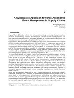
A Domain Engineering Process for RFID Systems Development in Supply Chain

105
device composed of microchip and an antenna attached to a substrate, as shown in Figure 1.
On the other hand, the RFID readers create a radio frequency field that detects radio waves.
When a tag passes through a radio frequency field generated by a compatible reader, the tag
reflects back to the reader the identifying information about the object to which it is
attached, thus identifying that object.


Fig. 1. Electronic Product Code and RFID Tag

Next, the EPC Middleware manages real-time read events and information, provides alerts,
and manages the basic read information for communication to EPC Information Services
and a company’s other existing information systems. The Discovery Services returm
locations that have some data related to an EPC (EPCglobal, 2005). In general, a Discovery
Services may contain pointers to entities other than the entity that originally assigned the
EPC code. Hence, Discovery Services are not universally authoritative for any data they may
have about an EPC. The important service in Discovery Services is the Object Name Service
(ONS) that, given an EPC, can return a list of network accessible service endpoints that
pertain to the EPC in question. Finally, the EPC Information Service (EPCIS) provides an
uniform programmatic interface to allow various clients to capture, secure, and access EPC-
related data and the business transactions which that data is associated (Harrison, 2003).
Companies that assign EPC numbers can maintain EPC Information Service servers with
item information. Using EPC numbers does not require organizations to share EPC data or
use other components of the system.
The EPCglobal Network presented previously contains several aspects that can be
considered by Software Reuse. According to (Harrison, 2003), the hardware, software, and
Interfaces defined in EPCglobal Network are management by applications with networked
databases. In this sense, software reuse can be used in development of applications, reusing
assets available in domains of the Supply Chain. For example, the localization of a product
in supply chain is divided into six steps: (i) the RFID reader capture the EPC stored on the
tag, (ii) EPC Middleware verify and validate the EPC, (iii) EPC Information Service search
data related to EPC in local ONS and return the result, (iv) next, the supply chain participant
authenticate it in the EPCglobal Network, (v) ONS search data related to EPC in external
databases using EPCglobal Network infrastructure, and (vi) return the search results to
application as shown in Figure 2.
This scenario and others situation are commons for some supply chain domains. Therefore,
the goal of domain engineering process described in this chapter is to identify common and
specific features, scenarios, domain-specific software architecture, and so on, for analysts
and designers in a domain, as well as simplifying the identification and implementation of
the software components.

The next section presents an analysis involving eleven software reuse processes discussing
their, fundamentals, concepts, pros and cons that consists a base for the process defined in
this chapter.