Systems, Structure and Control 2012 Part 4 docx

Asymptotic Stability Analysis of Linear Time-Delay Systems: Delay Dependent Approach

53
m
λ∈Σ (if it exists) as a solution of the system of equations (73), we arrive at maximal
solvent
m
R
.
Necessary condition. If system (67) is asymptotically stable, then
i
∀λ ∈Σ ,
i
1λ<
. Since
()
m
λ⊂Σ

R ,it follows that
()
m
1
ρ
<

R , therefore the positive definite solution of
Lyapunov matrix equation (67) exists.

Corollary 3.2.1 Suppose that for the given  , 1 N≤≤ , there exists matrix


R being
solution of SMPE (73). If system (67) is asymptotically stable, then matrix

R
is discrete
stable (
()
1
ρ
<

R ).
Proof. If system (67) is asymptotically stable, then zz1∀∈∑ < . Since
()
λ⊂∑

R , it
follows that
()
,1∀λ∈λ λ <

R , i.e. matrix

R is discrete stable.
Conclusion 3.2.1 It follows from the aforementioned, that it makes no difference which of
the matrices
m
R
, 1 N≤≤ we are using for examining the asymptotic stability of system
(67). The only condition is that there exists at least one matrix for at least one

 . Otherwise,
it is impossible to apply
Theorem 3.2.2.
Conclusion 3.2.2 The dimension of system (67) amounts to
(
)
j
N
jm
j1
e
Nnh1
=
=+
∑
.
Conversely, if there exists a maximal solvent, the dimension of
m
R is multiple times
smaller and amounts to
n

. That is why our method is superior over a traditional
procedure of examining the stability by eigenvalues of matrix
A .
The disadvantage of this method reflects in the probability that the obtained solution need
not be a maximal solvent and it can not be known ahead if maximal solvent exists at all.
Hence the proposed methods are at present of greater theoretical than of practical
significance.
3.2.4 Numerical example

Example 3.2.1
Consider a large-scale linear discrete time-delay systems, consisting of three
subsystems described by Lee, Radovic (1987)
( ) () () ( )
11 11 11 122 12
: x k 1 A x k B u k A x k h+= + + −S ,
( ) () () ( )
()
,
2 2 2 2 2 2 21 1 21 23 3 23
: xk1 Axk Buk Axkh Axkh+= + + − + −S
() () ()
()
33 33 33 311 31
: xk1 Axk Buk Axkh+= + + −S
,
,,,
12 112 2
0.7 0 0.5 0 0.1
0.8 0.6 0.1 0.1 0 0.1
A A 0.1 6 0.1 B A , B 0.1 0.2
0.4 0.9 0.1 0.1 0 0.1
0.6 1 0.8 0 0.1
−−
⎡
⎤⎡⎤
⎡⎤ ⎡⎤⎡ ⎤
⎢
⎥⎢⎥
==−−== =

⎢⎥ ⎢⎥⎢ ⎥
⎢
⎥⎢⎥
⎣⎦ ⎣⎦⎣ ⎦
⎢
⎥⎢⎥
−
⎣
⎦⎣⎦
,
,,,
21 23 3 3 31
0.1 0.2 0.1 0
1 0.1 0.1 0 0.1 0.2
A 0.3 0.1 A 0.2 0.2 , A B A
0.1 0.8 0 0.1 0.1 0.2
0.1 0.2 0.1 0
−− −
⎡⎤⎡⎤
⎡⎤⎡⎤⎡⎤
⎢⎥⎢⎥
==−===
⎢⎥⎢⎥⎢⎥
⎢⎥⎢⎥
−
⎣⎦⎣⎦⎣⎦
⎢⎥⎢⎥
⎣⎦⎣⎦
,
Systems, Structure and Control

54
The overall system is stabilized by employing a local memory-less state feedback control for
each subsystem
() ()
iii
uk Kxk= ,
[]
,,
12 3
74510 51
K67K K
444 14
−− −−
⎡
⎤⎡ ⎤
=− − = =
⎢
⎥⎢ ⎥
−− −
⎣
⎦⎣ ⎦

Substituting the inputs into this system, we obtain the equivalent closed loop system
representations
() ()
()
3
ii ii ijj ij
j1

ˆ
:x k 1 A x k Ax k h , 1 i 3
=
+= + − ≤≤
∑
S ,
iiii
ˆ
AABK=+
For time delay in the system, let us adopt:
12
h5= ,
21
h2= ,
23
h4= and
31
h5= . Applying
Theorem 3.2.1 to a given closed loop system, we obtain the following SMPE for 1=

65 3
1111221331
ˆ
ASASA0
−− −=RR R ,

65
12 122 12
ˆ
SSAA0

−−=RR ,

54
13 133 223
ˆ
SSASA0
−−=RR .
Solving this SMPE by minimization methods, we obtain
,
12 3
0.6001 0.3381 0.0922 1.3475 0.5264 0.6722 -0.3969
,S S
0.6106 0.3276 0.0032 1.3475 0.4374 1.3716 -1.0963
⎡⎤⎡ ⎤⎡ ⎤
== =
⎢⎥⎢ ⎥⎢ ⎥
⎣⎦⎣ ⎦⎣ ⎦
R .
Eigenvalue with maximal module of matrix
1
R equals 0.9382. Since eigenvalue
m
λ of
40 40×
∈A also has the same value, we conclude that solvent
1
R is maximal solvent
(
1m 1
=RR). Applying Theorem 3.2.2, we arrive at condition

()
1m
0.9382<1ρ=R
wherefrom we conclude that the observed closed loop large-scale time-delay system is
asymptotically stable.
The difference in dimensions of matrices

22
1
×
∈R and
40 40×
∈A is rather high, even
with relatively small time delays (the greatest time delay in our example is 5). So, in the case
of great time delays in the system and a great number of subsystems N , by applying the
derived results, a smaller number of computations are to be expected compared with a
traditional procedure of examining the stability by eigenvalues of matrix
A
.
An accurate number of computations for each of the mentioned method require additional
analysis, which is not the subject-matter of our considerations herein.
4. Conclusion
In this chapter, we have presented new, necessary and sufficient, conditions for the
asymptotic stability of a particular class of linear continuous and discrete time delay
systems. Moreover, these results have been extended to the large scale systems covering the
cases of two and multiple existing subsystems.
Asymptotic Stability Analysis of Linear Time-Delay Systems: Delay Dependent Approach

55
The time-dependent criteria were derived by Lyapunov’s direct method and are exclusively

based on the maximal and dominant solvents of particular matrix polynomial equation. It
can be shown that these solvents exist only under some conditions, which, in a sense, limits
the applicability of the method proposed. The solvents can be calculated using generalized
Traub’s or Bernoulli’s algorithms. Both of them possess significantly smaller number of
computation than the standard algorithm.
Improving the converging properties of used algorithms for these purposes, may be a
particular research topic in the future.
5. References
Boutayeb M., M. Darouach (2001) Observers for discrete-time systems with multiple delays,
IEEE Transactions on Automatic Control
, Vol. 46, No. 5, 746-750.
Boyd S., El Ghaoui L., Feron E., and Balakrishnan V. (1994)
Linear matrix inequalities in system
and control theory,
SIAM Studies in Applied Mathematics, 15. (Philadelphia, USA).
Chen J., and Latchman H.A. (1994) Asymptotic stability independent of delays: simple
necessary and sufficient conditions,
Proceedings of American Control Conference,
Baltimore, USA, 1027-1031.
Chen J., Gu G., and Nett C.N. (1994) A new method for computing delay margins for

stability of linear delay systems, Proceedings of 33rd IEEE Conference on Decision and
Control, Lake Buena Vista, Florida, USA, 433-437.
Chen J. (1995) On computing the maximal delay intervals for stability of linear delay
systems,
IEEE Transactions on Automatic Control, Vol. 40, 1087-1093.
Chiasson J. (1988) A method for computing the interval of delay values for which a
differential-delay system is stable,
IEEE Transactions on Automatic Control, 33, 1176-
1178.

Debeljkovic D.Lj., S.A. Milinkovic, S.B. Stojanovic (2005)
Stability of Time Delay Systems on
Finite and Infinite Time Interval, Cigoja press, Belgrade.
Debeljkovic Lj. D., S. A. Milinkovic (1999)
Finite Time Stability of Time Delay Systems, GIP
Kultura, Belgrade.
Dennis J. E., J. F. Traub, R. P. Weber (1976) The algebraic theory of matrix polynomials,
SIAM J. Numer. Anal., Vol. 13 (6), 831-845.
Dennis J. E., J. F. Traub, R. P. Weber (1978) Algorithms for solvents of matrix polynomials,
SIAM J. Numer. Anal., Vol. 15 (3), 523-533
Fridman E. (2001) New Lyapunov–Krasovskii functionals for stability of linear retarded and
neutral type systems,
Systems and Control Letters, Vol. 43, 309–319.
Fridman E. (2002) Stability of linear descriptor systems with delay: a Lyapunov-based
approach,
Journal of Mathematical Analysis and Applications, 273, 24–44.
Fridman E., and Shaked U. (2002a) A descriptor system approach to H∞ control of linear
time-delay systems,
IEEE Transactions on Automatic Control, Vol. 47, 253–270.
Fridman E., and Shaked U. (2002b) An improved stabilization method for linear time-delay
systems,
IEEE Transactions on Automatic Control, Vol. 47, 1931–1937.
Fridman E., and Shaked U. (2003) Delay-dependent stability and H∞ control: Constant and
time-varying delays,
International Journal of Control, Vol. 76, 48–60.
Fridman E., and Shaked U. (2005) Delay-Dependent H∞ Control of Uncertain Discrete Delay
Systems,
European Journal of Control , Vol. 11, 29–37.
Systems, Structure and Control

56
Fu M., Li H., and Niculescu S I. (1997) Robust stability and stabilization of time-delay system via
integral quadratic constraint approach
. In L. Dugard and E. I. Verriest (Eds.), Stability
and Control of Time-Delay Systems, LNCIS, 228, (London: Springer-Verlag), 101-
116.
Gantmacher F. (1960)
The theory of matrices, Chelsea, New York.
Gao H., Lam J., Wang C. and Wang Y. (2004) Delay dependent output-feedback stabilization
of discrete time systems with time-varying state delay,
IEE Proc Control Theory A,
Vol. 151, No. 6, 691-698.
Golub G.H., and C.F. Van Loan, (1996)
Matrix computations, Jons Hopkins University Press,
Baltimore.
Gorecki H., S. Fuksa, P. Grabovski and A. Korytowski (1989)
Analysis and synthesis of time
delay systems
, John Wiley & Sons, Warszawa.
Goubet-Bartholomeus A., Dambrine M., and Richard J P. (1997) Stability of perturbed
systems with time-varying delays,
Systems and Control Letters, Vol. 31, 155- 163.
Gu K. (1997) Discretized LMI set in the stability problem of linear uncertain time-delay
systems,
International Journal of Control, Vol. 68, 923-934.
Hale J.K. (1977)
Theory of functional differential equations (Springer- Verlag, New York,
Hale J.K., Infante E.F., and Tsen F.S.P. (1985) Stability in linear delay equations,
Journal on
Mathematical Analysis and Applications

, Vol. 105, 533-555.
Hale J.K., and Lunel S.M. (1993)
Introduction to Functional Differential Equations, Applied
Mathematics Sciences Series
, 99, (New York: Springer-Verlag).
Han Q L. (2005a) On stability of linear neutral systems with mixed time-delays: A
discretized Lyapunov functional approach,
Automatica Vol. 41, 1209–1218.
Han Q L. (2005b) A new delay-dependent stability criterion for linear neutral systems with
norm-bounded uncertainties in all system matrices,
Internat. J. Systems Sci., Vol. 36,
469–475.
Hertz D., Jury E. I., and Zeheb E. (1984) Stability independent and dependent of delay for
delay differential systems.
Journal of Franklin Institute, 318, 143-150.
Hu Z. (1994) Decentralized stabilization of large scale interconnected systems with delays,

IEEE Transactions on Automatic Control, Vol. 39, 180-182.
Huang S., H. Shao, Z. Zhang (1995) Stability analysis of large-scale system with delays,
Systems & Control Letters, Vol. 25, 75-78.
Kamen E.W. (1982) Linear systems with commensurate time delays: Stability and
stabilization independent of delay.
IEEE Transactions on Automatic Control, Vol. 27,
367-375; corrections in
IEEE Transactions on Automatic Control, Vol. 28, 248-249,
1983.
Kapila V., Haddad W. (1998) Memoryless H∞ controllers for discrete-time systems with
time delay,
Automatica, Vol. 34, 1141-1144.
Kharitonov V. (1998) Robust stability analysis of time delay systems: A survey,

Proceedings of
4th IFAC System Structure and Control Conference, Nantes, France, July.
Kim H. (2000) Numerical methods for solving a quadratic matrix equation,
Ph.D. dissertation,
University of Manchester, Faculty of Science and Engineering.
Kim H. (2001) Delay and its time-derivative dependent robust stability of time delayed
linear systems with uncertainty,
IEEE Transactions on Automatic Control 46 789–792.
Asymptotic Stability Analysis of Linear Time-Delay Systems: Delay Dependent Approach

57
Kolla S. R., J. B. Farison (1991) Analysis and design of controllers for robust stability of
interconnected continuous systems,
Proceedings Amer. Contr. Conf., Boston, MA,
881-885.
Kolmanovskii V. B., and Nosov V. R. (1986) Stability
of Functional Differential Equations (New
York: Academic Press)
Kolmanovskii V., and Richard J. P. (1999) Stability of some linear systems with delays.
IEEE
Transactions on Automatic Control
, 44, 984–989.
Kolmanovskii V., Niculescu S I., and Richard J. P., (1999) On the Lyapunov–Krasovskii
functionals for stability analysis of linear delay systems.
International Journal of
Control
, Vol. 72, 374–384.
Lakshmikantam V., and Leela S. (1969)
Differential and integral inequalities (New York:
Academic Press).

Lancaster P., M. Tismenetsky (1985)
The theory of matrices, 2nd Edition, Academic press, New
York.
Lee C., and Hsien T. (1997) Delay-independent Stability Criteria for Discrete uncertain
Large-scale Systems with Time Delays,
J. Franklin Inst., Vol. 33 4B, No. 1, 155-166.
Lee T.N., and Radovic U. (1987) General decentralized stabilization of large-scale linear
continuous and discrete time-delay systems,
Int. J. Control, Vol. 46, No. 6, 2127-2140.
Lee T.N., and Radovic U. (1988) Decentralized Stabilization of Linear Continuous and
Discrete-Time Systems with Delays in Interconnections,
IEEE Transactions on
Automatic Control
, Vol. 33, 757–761.
Lee T.N., and S. Diant (1981) Stability of time-delay systems,
IEEE Transactions on Automatic
Control, Vol. 26, No. 4, 951-953.
Lee Y.S., and Kwon W.H. (2002) Delay-dependent robust stabilization of uncertain discrete-
time state-delayed systems.
Preprints of the 15
th
IFAC World Congress, Barcelona,
Spain,
Li X., and de Souza, C. (1995) LMI approach to delay dependent robust stability and
stabilization of uncertain linear delay systems.
Proceedings of 34th IEEE Conference
on Decision and Control, New Orleans, Louisiana, USA, 3614-3619.
Li X., and de Souza, C. (1997) Criteria for robust stability and stabilization of uncertain linear
systems with state delay,
Automatica, Vol. 33, 1657–1662.

Lien C H., Yu K W., and Hsieh J G., (2000) Stability conditions for a class of neutral
systems with multiple time delays.
Journal of Mathematical Analysis and Applications,
245, 20–27.
Mahmoud M, Hassen M, and Darwish M. (1985)
Large-scale control system: theories and
techniques
. New York: Marcel-Dekker.
Mahmoud M. (2000) Robust H∞ control of discrete systems with uncertain parameters and
unknown delays,
Automatica Vol. 36, 627-635.
Malek-Zavarei M., and Jamshidi M. (1987)
Time-Delay Systems, Analysis, Optimization and
Applications, Systems and Control Series, Vol. 9 (North-Holland).
Moon Y.S., Park P.G., Kwon W.H., and Lee Y.S. (2001). Delay-dependent robust stabilization
of uncertain state-delayed systems,
International Journal of Control, Vol. 74(14), 1447–
1455.
Niculescu S I., de Souza C. E., Dion J M., and Dugard L., (1994), Robust stability and
stabilization for uncertain linear systems with state delay: Single delay case (I).
Proceedings of IFAC Workshop on Robust Control Design, Rio de Janeiro, Brazil, 469-474.
Systems, Structure and Control

58
Niculescu S I., de Souza C. E., Dugard L., and Dion J M. (1995a), Robust exponential
stability of uncertain linear systems with time-varying delays.
Proceedings of 3rd
European Control Conference
, Rome, Italy, 1802-1807.
Niculescu S I., Trofino-Neto A., Dion J M., and Dugard L. (1995b), Delay-dependent

stability of linear systems with delayed state: An L.M.I. approach.
Proceedings of
34th IEEE Conference on Decision and Control
, New Orleans, Louisiana, USA, 1495-
1497.
Niculescu S I., Dion J M., Dugard L., and Li H. (1997a) Stability of linear systems with
delayed state: An L.M.I. approach. JESA,
special issue on “Analysis and control of time-
delay systems”
, 31, 955-970.
Niculescu S.I., Verriest E. I., Dugard L., and Dion J. M. (1997b)
Stability and robust stability of
time-delay systems: A guided tour. Lecture notes in control and information sciences
, Vol.
228 ( 1–71). London: Springer.
Niculescu S I., (2001), On delay-dependent stability under model transformations of some
neutral linear systems,
International Journal of Control, Vol. 74, 609–617.
Niculescu S.I., and Richard J.P. (2002) Analysis and design of delay and propagation systems,
IMA Journal of Mathematical Control and Information, 19(1–2), 1–227 (special issue).
Oucheriah S. (1995) Measure of robustness for uncertain time-delay linear system,
ASME
Journal of Dynamic Systems, Measurement, and Control 117 633–635.
Park J.H. (2002) Robust Decentralized Stabilization of Uncertain Large-Scale Discrete-Time
Systems with Delays,
Journal of Optimization Theory and Applications, Vol. 113, No. 1,
105–119.
Park J.H. (2004) Robust non-fragile control for uncertain discrete-delay large-scale systems
with a class of controller gain variations,
Applied Mathematics and Computation, Vol.

149, 147–164.
Park J.H., Jung Ho Y., Park J.I., Lee S.G. (2004) Decentralized dynamic output feedback
controller design for guaranteed cost stabilization of large-scale discrete-delay
systems,
Applied Mathematics and Computation, Vol. 156, No 2, 307-320.
Park P., Moon Y S., & Kwon W H. (1998) A delay-dependent robust stability criterion for
uncertain time-delay systems,
In Proceedings of the American control conference, 1963–
1964.
Park P. (1999) A delay-dependent stability criterion for systems with uncertain time-
invariant delays.
IEEE Transactions on Automatic Control, Vol. 44, 876–877.
Pereira E. (2003) On solvents of matrix polynomials,
Applied numerical mathematics, Vol. 47,
197-208.
Richard J P., Goubet- Bartholomeus A., Tchangani, Ph. A., and Dambrine M. (1997)
Nonlinear delay systems: Tools for quantitative approach to stabilization. L. Dugard and E.
I. Verriest, (Eds.), Stability and Control of Time-Delay Systems
, LNCIS, 228, (London:
Springer-Verlag), 218-240.
Richard J P. (1998) Some trends and tools for the study of time delay systems.
Proceedings of
CESA98 IMACS/IEEE Multi conference, Hammamet, Tunisia, 27-43.
Richard J.P. (2003) Time-delay systems: an overview of some recent advances and open
problems,
Automatica Vol. 39, 1667–1694.
Shi P., Agarwal R.K., Boukas E K., Shue S P. (2000) Robust H∞ state feedback control of
discrete timedelaylinear systems with norm-bounded uncertainty,
Internat. J.
Systems Sci., Vol. 31 409- 415.

Asymptotic Stability Analysis of Linear Time-Delay Systems: Delay Dependent Approach

59
Siljak D. (1978) Large-scale dynamic systems: stability and structure, Amsterdam: North
Holland.
Song S., Kim J., Yim C., Kim H. (1999) H∞ control of discrete-time linear systems with time-
varying delays in state,
Automatica Vol. 35, 1587-1591.
Stojanovic S.B., Debeljkovic D.Lj. (2005) Necessary and Sufficient Conditions for Delay-
Dependent Asymptotic Stability of Linear Continuous Large Scale Time Delay
Autonomous Systems,
Asian Journal of Control, Vol. 7, No. 4, 414 - 418.
Stojanovic S.B., Debeljkovic D.Lj. (2006) Comments on Stability of Time-Delay Systems,

IEEE Transactions on Automatic Control
(submitted).
Stojanovic S.B., Debeljkovic D.Lj. (2008.a) Delay–Dependent Stability of Linear Discrete
Large Scale Time Delay Systems: Necessary and Sufficient Conditions,
International
Journal of Information & System Science
, Vol. 4, No. 2, 241 – 250.
Stojanovic S.B., Debeljkovic D.Lj. (2008.b) Necessary and Sufficient Conditions for Delay-
Dependent Asymptotic Stability of Linear Discrete Time Delay Autonomous
Systems,
Proceedings of 17th IFAC World Congress, Seoul, Korea, July 06–10.
Su J.H. (1994) Further results on the robust stability of linear systems with a single delay,
Systems and Control Letters, Vol. 23, 375-379.
Su J.H. (1995) The asymptotic stability of linear autonomous systems with commensurate
delays.
IEEE Transactions on Automatic Control, Vol. 40, 1114-1118.

Suh H., Z. Bein (1982) On stabilization by local state feedback for continuous-time large-
scale systems with delays in interconnections,
IEEE Transactions on Automatic
Control, Vol. AC-27, 964-966.
Trinh H., and Aldeen M. (1995a) A Comment on Decentralized Stabilization of Large-Scale
Interconnected Systems with Delays,
IEEE Transactions on Automatic Control, Vol.
40, 914–916.
Trinh H., M. Aldeen (1995b) A comment on Decentralized stabilization of large scale
interconnected systems with delays,
IEEE Transactions on Automatic Control, Vol. 40,
914-916.
Trinh H., M. Aldeen (1997) On Robustness and Stabilization of Linear Systems with Delayed
Nonlinear Perturbations,
IEEE Transactions on Automatic Control, Vol. 42, 1005-1007.
Verriest E., Ivanov A. (1995) Robust stability of delay difference equations,
Proceedings
IEEEE Conf. on Dec. and Control, New Orleans, LA 386-391.
Verriest E., and Niculescu S I. (1998)
Delay-independent stability of linear neutral systems: a
Riccati equation approach. In L. Dugard and E. Verriest (eds) Stability and Control of
Time-Delay Systems
, Vol. 227 (London: Springer-Verlag), 92–100.
Wang W. J., R. J. Wang, and C. S. Chen (1995) Stabilization, estimation and robustness for
continuous large scale systems with delays,
Contr. Theory Advan. Technol., Vol. 10,
No. 4, 1717-1736.
Wang W. and, L. Mau (1997) Stabilization and estimation for perturbed discrete time-delay
large-scale systems,
IEEE Transactions on Automatic Control, Vol. 42, No. 9, 1277-

1282.
Wu H. and K. Muzukami (1995) Robust stability criteria for dynamical systems in delayed
perturbations,
IEEE Transactions on Automatic Control, Vol. 40, 487–490.
Wu H. (1999) Decentralized Stabilizing State Feedback Controllers for a Class of Large-Scale
Systems Including State Delays in the Interconnections,
Journal of optimization theory
and applications, Vol. 100. No. 1, 59-87.
Systems, Structure and Control

60
Xu B. (1995) On delay-Independent and stability of large-scale systems with time delays,
IEEE Transactions on Automatic Control
, Vol. 40, 930-933.
Xu B., (1994) Comments on robust stability of delay dependence for linear uncertain
systems,
IEEE Transactions on Automatic Control, Vol. 39 2365.
Xu S., Lam J., and Yang C. (2001) H∞ and positive real control for linear neutral delay
systems,
IEEE Transactions on Automatic Control, Vol. 46, 1321–1326
Yan J.J. (2001) Robust stability analysis of uncertain time delay systems with delay-
dependence,
Electronics Letters Vol. 37, 135–137.

3
Differential Neural Networks Observers:
development, stability analysis and
implementation
Alejandro García
1

, Alexander Poznyak
1
, Isaac Chairez
2

and Tatyana Poznyak
2

1
Department of Automatic Control, CINVESTAV-IPN,
2
Superior School of Chemical Engineering National Polytechnic Institute (ESIQIE-IPN)
México
1. Introduction
The control and possible optimization of a dynamic process usually requires the complete
on-line availability of its state-vector and parameters. However, in the most of practical
situations only the input and the output of a controlled system are accessible: all other
variables cannot be obtained on-line due to technical difficulties, the absence of specific
required sensors or cost (Radke & Gao, 2006). This situation restricts possibilities to design
an effective automatic control strategy. To this matter many approaches have been proposed
to obtain some numerical approximation of the entire set of variables, taking into account
the current available information. Some of these algorithms assume a complete or partial
knowledge of the system structure (mathematical model). It is worth mentioning that the
influence of possible disturbances, uncertainties and nonlinearities are not always
considered.
The aforementioned researching topic is called state estimation, state observation or, more
recently, software sensors design. There are some classical approaches dealing with same
problem. Among others there are a few based on the Lie-algebraic method (Knobloch et. al.,
1993), Lyapunov-like observers (Zak & Walcott, 1990), the high-gain observation (Tornambe
1989), optimization-based observer (Krener & Isidori 1983), the reduced-order nonlinear

observers (Nicosia et. al.,1988), recent structures based on sliding mode technique (Wang &
Gao, 2003), numerical approaches as the set-membership observers (Alamo et. al., 2005) and
etc. If the description of a process is incomplete or partially known, one can take the
advantage of the function approximation capacity of the Artificial Neural Networks (ANN)
(Haykin, 1994) involving it in the observer structure designing (Abdollahi et. al., 2006),
(Haddad, et. al. 2007), (Pilutla & Keyhani, 1999).
There are known two types of ANN: static one, (Haykin, 1994) and dynamic neural networks
(DNN). The first one deals with the class of global optimization problems trying to adjust
the weights of such ANN to minimize an identification error. The second approach,
exploiting the feedback properties of the applied Dynamic ANN, permits to avoid many
problems related to global extremum searching. Last method transforms the learning
process to an adequate feedback design (Poznyak et. al., 2001). Dynamic ANN’s provide an
Systems, Structure and Control

62
effective instrument to attack a wide spectrum of problems, such as parameter
identification, state estimation, trajectories tracking, and etc. Moreover, DNN demonstrates
remarkable identification properties in the presence of uncertainties and external
disturbances or, in other words, provides the robustness property.
In this chapter, we discuss the application of a special type of observers (based on the DNN)
for the state estimation of a class of uncertain nonlinear system, which output and state are
affected by bounded external perturbations. The chapter comprises four sections. In the first
section the fundamentals concerning state estimation are included. The second section
introduces the structure of the considered class of Differential Neural Network Observers
(DNNO) and their main properties. In the third section the main result concerning the
stability of estimation error, with its analysis based on the Lyapunov-Like method and
Linear Matrix Inequalities (LMI) technique is presented. Moreover, the DNN dynamic
weights boundedness is stated and treated as a second level of the learning process (the first
one is the learning laws themselves). In the last section the implementation of the suggested
technique to the chemical soil treatment by ozone is considered in details.

2. Fundamentals
2.1 Estimation problem
Consider the nonlinear continuous-time model given by the following ODE:

()()
η(t)Cx(t)y(t)
) x(ξ(t),tux(t),fx(t)
dt
d
+=
+= fixed is0
(1)
where
n
x(t) ℜ∈

- state-vector at time 0t ≥ ,
m
y(t) ℜ∈

- corresponding measurable
output,
nm
C
×
ℜ∈

- the known matrix defining the
state-output transformation,
()

r
tu ℜ∈

- the bounded control action
()
nr ≤
belonging to the
following admissible set
() ()
{}
∞<ϒ≤=
u
tu:tu:U
adm
,
ξ(t) and η(t)
- noises in the state dynamics and
in the output, respectively,
nrn
:f
ℜ→
×
ℜ .
The software sensor design, also called state estimation (observation) problem, consists in
designing a vector-function
n
(t)x
ˆ
ℜ∈ , called “estimation vector”, based only the available
data information (measurable)

()
{}
[]
t,τ
u(t),ty
0∈
in such a way that it would be "closed" to
its real (but non-measurable) state-vector x(t). The measure of that "closeness" depends on
the accepted assumptions on the state dynamics as well as the noise effects. The most of
observers usually have ODE-structure:
Differential Neural Networks Observers: development, stability analysis and implementation

63

()
[]
vectorfixed a is ,
0
ˆ
0
ˆˆ
x t,
t,τ
y,tu(t),xF(t)x
dt
d
⎟
⎠
⎞
⎜

⎝
⎛
∈
=
(2)
Here the mapping
nm
L
rn
:F
ℜ→
+
ℜ××ℜ×ℜ defines the structure of the observer to be
implemented.
2.2 Physical Constraints of the state vector
To realize the state observation objective, many authors have taken advantages of the
physical state constraints. Some examples of these techniques employing “
a priori”
information on states are: interval observers (Dochain, 2003) and moving horizon state
estimation (Valdes-González et. al., 2003). In the present study, some physical restrictions
are considered and using previous results given in (García, et. al. 2007). The main property
of an observer, which are looked for, is to keep the generated state estimates
(t)x
ˆ
within the
given compact set
X
(even in the presence of noise), that is:

X(t)x ∈

ˆ
(3)
In different problems the
compact set
X
has a concrete physical sense. For example, the
dynamic behaviors of some reagents, participating in chemical reactions, always keep their
nonnegative current values. Similar remark seems to be true for other physical variables
such as temperature, pressure, light intensity and etc. To complete (3) the next
projectional
observer
is proposed:

()
()
[]
)h( t,dττ,
τ,s
y,τu,)(x
ˆ
F
t
thtτ
h(t))(tx
ˆ
X
π(t)x
ˆ
0
0

>
⎪
⎭
⎪
⎬
⎫
⎪
⎩
⎪
⎨
⎧
⎟
⎠
⎞
⎜
⎝
⎛
∈
∫
−=
+−=
τ
(4)
Here
()
1
Cth ∈ fulfills
()
0≤th


. The operator
{}
⋅
X
π is the projector to the given convex
compact set
X
possessing the property

{}
zxzx
X
π −≤− (5)
for any
n
x ℜ∈ and any Xz∈ . The operator
{}
⋅
X
π may be defined by different ways.
Two examples of
{}
⋅
X
π
are given below.
Example 1 (Saturation function):

{}
(

)
Τ
⎥
⎦
⎤
⎢
⎣
⎡
⎟
⎠
⎞
⎜
⎝
⎛
=
n
xsatxsatx
X
π …
1
(6)
where for any i=1 n

⎪
⎪
⎩
⎪
⎪
⎨
⎧

+
≥
+
+
<<
−
−
≤
−
=
)
i
(x
i
x)
i
(x
)
i
(x
i
x)
i
(x
i
x
)
i
(x
i

x)
i
(x
):
i
sat(x
(7)
Systems, Structure and Control

64
with
+
<
−
)
i
(x)
i
(x
as an extreme point a priori known.
Example 2 (Simplex): If X is the n-simplex, i.e.,

()
⎭
⎬
⎫
⎩
⎨
⎧
∑≥

==∈=
=
11
1
0
i
n
i
i
n
zn, ,iRzX , z: (8)
then
{}
x
X
π can be found numerically by at least within n-steps. The case 3n = is
illustrated by Figure 1.

Figure 1. Projectional operator over a simplex (n=3)
An important point is that with the projectional operator implementations the trajectories
(){}
tx
ˆ
, generated by (4), are not differentiable for any 0>≥ h(t)t .
3 Structures of DNN Observers
3.1 State estimation under complete information
If the right-hand side
()
x(t)f of the dynamics (1) is known then the structure
F

of the
observer (4) is usually selected in the, so-called, Luenberger-type form:

() ()
()()
()
()
(t)x
ˆ
Cy(t)tKu(t)(t),x
ˆ
ft,ty,tu(t),x
ˆ
F −+= (9)
So, it repeats the dynamics of the plant and, additionally, contains the correction term,
proportional to the output error (see, for example Yaz & Azemi, 1994; Poznyak, 2004). The
adequate selection of the matrix-gain
()
tK provides a good-enough state estimation.
3.2 Differential Neural Network Observer, the "grey-box" case
In the case when the right-hand side
()
ux,f
of the dynamics (1) is unknown, there is
suggested to apply some guessing of it, say,
()
W(t)|u(t)x(t),f
where
n
f ℜ∈

defines the
approximating map depending on the time-varying parameters
W(t) , which should be
adjusted by a "
adaptation law" suggested by a designer or derived, using some stability
Differential Neural Networks Observers: development, stability analysis and implementation

65
analysis method. According to the DNN-approach (Poznyak et. al., 2001) we may
decompose
()
W(t)|u(t)x(t),f in two parts: first one, approximates the linear dynamics part
by a
Hurwitz fixed matrix
nn
A
×
ℜ∈
(selected by the designer) and the second one, uses
the ANN reconstruction property for the nonlinear part by means of variable time
parameters
(t)
,
W
21
with a set of basis functions, that is,

() ()
()
()

rq
,
qn
(t)W
p
σ,
pn
(t) W,
nn
A
u(t)x(t)(t)Wx(t)(t)σWAx(t):(t)
,
W|u(t)x(t),f
×
ℜ∈⋅
×
ℜ∈
×
ℜ∈⋅
×
ℜ∈
×
ℜ∈
++=
⎟
⎠
⎞
⎜
⎝
⎛

ϕ
ϕ
2
1
1
2121
(10)
The activation vector (the basis) function
()
⋅σ and matrix-function
()
⋅
ϕ
are usually
selected as functions with
sigmoid-type components, i.e.:

()
n, j,(t)
j
x
j
c
n
j
exp
j
b
j
a:x(t)

j
σ 1
1
1
1 =
−
⎟
⎟
⎟
⎠
⎞
⎜
⎜
⎜
⎝
⎛
⎟
⎟
⎟
⎠
⎞
⎜
⎜
⎜
⎝
⎛
∑
=
−+=
(11)

and

()
r,j;q, i,(t)
s
x
si,
c
n
s
exp
ji,
b
ji,
a:x(t)
ji,
11
1
1
1 ==
−
⎟
⎟
⎠
⎞
⎜
⎜
⎝
⎛
⎟

⎟
⎠
⎞
⎜
⎜
⎝
⎛
∑
=
−+=
ϕ
(12)
It is easy to see that the activation functions satisfy the following sector conditions

()
()
22
σ
Λ
(t)xx(t)
σ
L
σ
Λ
(t)xσx(t)σ
′
−≤
′
−
(13)

()
()
22
ϕ
ϕ
ϕ
ϕϕ
Λ
(t)xx(t)L
Λ
(t)xx(t)
′
−≤
′
−
(14)
and stay bounded on
n
ℜ
. In (10), the constant parameter A , as well as the time-varying
parameters
(t)
,
W
21
, should be properly adjusted to guarantee a good state approximation.
Notice that for any fixed matrices
2121 ,
W

ˆ
(t)
,
W =
the dynamics (1) always could be
represented as

() ()
()
⎟
⎠
⎞
⎜
⎝
⎛
−=
++++=
21
21
,
W
ˆ
|x(t)fx(t)f:(t)f
~
ξ(t)(t)f
~
u(t)x(t)W
ˆ
x(t)σW
ˆ

Ax(t)x(t)
dt
d
ϕ
(15)
Systems, Structure and Control

66
where
()
tf
~
is referred to as a modeling error vector-field called the "unmodelled dynamics".
In view of the corresponding boundedness property, the following inequality for the
unmodelled dynamics

()
tf
~
takes place:

T
f
~
Λ
f
~
Λ,
T
f

Λ
f
Λ,
f
~
Λ,
f
Λ;f
~
,f
~
f
~
Λ
x(t)f
~
f
~
f
Λ
(t)f
~
⎟
⎠
⎞
⎜
⎝
⎛
==>>
+≤

11
0
1
0
10
2
1
10
2
(16)
3.3 Structure DNN observers considering state physical constraints
Introduce the following projectional DNNO:

()
() ()
[]
)t(x
ˆ
C)t(y:)t(e
d)(Ke)(u)(x)((W)(x
ˆ
)(W)(x
ˆ
A
t
tht
))t(ht(x
ˆ
X
)t(x

ˆ
−=
⎪
⎭
⎪
⎬
⎫
⎪
⎩
⎪
⎨
⎧
+++
∫
−=
−
ττττϕττσττ
τ
π
21
+=
(17)
Here the weights matrices
()
tW
1
and
()
tW
2

supply the adaptive behavior to this class of
observers if they are adjusted by an adequate manner. We derived (see Appendix) the
following nonlinear weight
updating laws based on the Lyapunov-like stability analysis:

() () ()
()
⎪
⎪
⎪
⎭
⎪
⎪
⎪
⎬
⎫
⎟
⎠
⎞
⎜
⎝
⎛
+
⎟
⎠
⎞
⎜
⎝
⎛
Λ+Λ=Π

−=−+Π=Ω
−Ω
−
−=
IPNC
T
CN
;W
ˆ
)t(W:)t(W
~
; ))t(ht(e
T
CN)t(x
ˆ
)t(W
~
:)t(
tW
~
dt
)t(dk
)t(x
ˆ
T
)t(P
)t(k
tW
dt
d

ϖ
ϖ
ϖ
ϖ
σ
σ
23
111
2
1
1
2
1
1
1
(18)

() ()() ()
()
⎪
⎪
⎪
⎭
⎪
⎪
⎪
⎬
⎫
⎟
⎠

⎞
⎜
⎝
⎛
+
⎟
⎠
⎞
⎜
⎝
⎛
Λ+Λ=Ξ
−=−+Ξ=Φ
−Φ
−
−=
IPNC
T
CN
;W
ˆ
)t(W:)t(W
~
; ))t(ht(e
T
CN)(u)(x
ˆ
)((W
~
:)t(

tW
~
dt
)t(dk
x
ˆ
T
)(
T
u)t(P
)t(k
tW
dt
d
ϖ
ϖ
ϖ
ϖ
ττϕτ
τϕτ
67
222
2
2
2
2
2
1
2
2

(19)
where:
0
1
>
−
⎟
⎠
⎞
⎜
⎝
⎛
+=
ϖϖ
ϖ
,IC
T
CN
To improve the behavior of this adaptive laws, the matrix
21,
W
ˆ
can be "provided" by one
of the, so-called, training algorithms (see, for example, Chairez et. al., 2006; Stepanyan &
Hovakimyan, 2007). Both present least square solutions considering some identification
structure for possible set of fictitious values or even an available set of directly measured
data of the process.
Differential Neural Networks Observers: development, stability analysis and implementation

67

4. DNN Observers Stability
4.1 Behavior of weights dynamics
Here we wish to show that under the adapting weights laws (18) and (19) the weights
()
tW
1
and
()
tW
2
are bounded.
Theorem 1 (bounded adaptive weights): If (t)
i
k
()
21,i = in (18) and (19) satisfy

()
()
() ( )
{
}
() ()
{}
() ()
[]
()
() ()()
{}
() ()

{}
⎟
⎠
⎞
⎜
⎝
⎛
−+
Φ
−≤
−+
Ω
−≤
min,
k)t(k)t(cktW
~
T
tW
~
tr
tx
ˆ
T
)t(
T
u)t(PtW
~
tr)t(k
)t(k
dt

d
min
ktktcktW
~
t
T
W
~
tr
)t(x
ˆ
T
)t(Pt
T
W
~
trtk
)t(k
dt
d
22
222
2
2
2
2
2
11111
1
2

1
2
1
ϕ
σ
(20)
then
() ()
{
}
tW
~
t
T
W
~
tr
11
is monotonically non-increasing function.
Proof: Considering the dynamics for the weight matrix
()
tW
~
1
and the following candidate
Lyapunov function
()
.t
w
V

() () ()
{}
()
[]
2
11
4
11
2
1
+
−+=
min
ktk
c
tW
~
t
T
W
~
tr:t
w
V
(21)
where

()
[]

() ()
()
⎩
⎨
⎧
<
≥
=
+
00
0
tz
tztz
:tz
(22)
Then, one has

() () ()
()
()
[]
2
11
1
1
11
2
+
−
−+

⎪
⎭
⎪
⎬
⎫
⎪
⎩
⎪
⎨
⎧
⎟
⎟
⎟
⎠
⎞
⎜
⎜
⎜
⎝
⎛
=
min
T
w
ktk
dt
)tk(d
ctW
dt
d

tW
~
tr:tV
dt
d
(23)
By (18) it follows

() ()
()
() ()
()
[]
()
() ( )
{}
() () ()
{}
()
[]
⎟
⎠
⎞
⎜
⎝
⎛
+
−
−
+

−−
+Ω
−
≤
+
−
−
+
⎪
⎭
⎪
⎬
⎫
⎪
⎩
⎪
⎨
⎧
⎟
⎟
⎟
⎠
⎞
⎜
⎜
⎜
⎝
⎛
⎥
⎦

⎤
⎢
⎣
⎡
−Ω
−
−=
min
ktkctW
~
t
T
W
~
trtk
d
t
))t(k(d
)t(x
ˆ
T
)t(Pt
T
W
~
tr
tk
min
ktk
dt

))t(k(d
c
tW
~
dt
))t(k(d
)t(x
ˆ
T
)t(P
tk
t
T
W
~
trt
w
V
dt
d
11
1
2
11
1
1
1
1
2
1

2
1
11
1
1
2
1
1
2
1
1
1
σ
σ
(24)
The property
()
0t
w
V
dt
d
≤
results from (20).
Some examples of
)t(
i
k
()
21,i = are given below

Systems, Structure and Control

68
a. Introduce the following auxiliary function
() ()()
() () ( )
{}
()
+
⎥
⎦
⎤
⎢
⎣
⎡
−
Ω
−
=
⎟
⎠
⎞
⎜
⎝
⎛
−
min,
ktkc
)t(x
ˆ

T
)t(Pt
T
W
~
trtk
:thte,t
T
W
~
s
11
1
1
1
1
σ

And select
()
()
()
⎟
⎠
⎞
⎜
⎝
⎛
−−<
⎟

⎠
⎞
⎜
⎝
⎛
⎟
⎠
⎞
⎜
⎝
⎛
−+
⎟
⎠
⎞
⎜
⎝
⎛
−
−=
>+
⎟
⎠
⎞
⎜
⎝
⎛
−+
=
))t(ht(e),t(

T
W
~
s
t
j
bexp))t(ht(e),t(
T
W
~
a
btexp
j
b))t(ht(e),t(
T
W
~
a
)(k:
dt
))t(
k(d
jmin,
k ,
jmin,
k
btexp))t(ht(e),t(
T
W
~

a
)(k
:tk
1
1
1
1
0
1
1
0
1
1
0
1

Leading to
()
⎟
⎠
⎞
⎜
⎝
⎛
−>
⎟
⎠
⎞
⎜
⎝

⎛
⎟
⎠
⎞
⎜
⎝
⎛
−−
⎟
⎠
⎞
⎜
⎝
⎛
−
))t(ht(e),t(
T
W
~
s
))t(ht(e),t(
T
W
~
sb)(kbtexp))t(ht(e),t(
T
W
~
a
1

1
0
1

The last inequality is fulfilled if the weight dependent parameter
⎟
⎠
⎞
⎜
⎝
⎛
e(t))(t),
T
W
~
a
1
is selected
as
()
⎟
⎠
⎞
⎜
⎝
⎛
−−=Ψ
−
Ψ−
⎟

⎠
⎞
⎜
⎝
⎛
−>
⎟
⎠
⎞
⎜
⎝
⎛
−
))t(ht(e),t(
T
W
~
sb)(k:
btexp))t(ht(e),t(
T
W
~
s))t(ht(e),t(
T
W
~
a
1
0
1

11

b. Analogously, for
()
t
T
W
~
2
:
() ()()
() () ( )()
{}
()
+
⎥
⎦
⎤
⎢
⎣
⎡
−
Φ
−
=
⎟
⎠
⎞
⎜
⎝

⎛
−
min,
ktkc
x
ˆ
T
)(
T
u)t(Pt
T
W
~
trtk
:thte,t
T
W
~
s
22
2
1
2
2
τϕτ

()
()
()
⎟

⎠
⎞
⎜
⎝
⎛
−−<
⎟
⎠
⎞
⎜
⎝
⎛
⎟
⎠
⎞
⎜
⎝
⎛
−+
⎟
⎠
⎞
⎜
⎝
⎛
−
−=
>+
⎟
⎠

⎞
⎜
⎝
⎛
−+
=
))t(ht(e),t(
T
W
~
s
t
j
bexp))t(ht(e),t(
T
W
~
a
btexp
j
b))t(ht(e),t(
T
W
~
a
)(k:)t(k
dt
d
jmin,
k ,

jmin,
k
btexp))t(ht(e),t(
T
W
~
a
)(k
:tk
2
2
1
2
0
22
0
2
1
0
2

Differential Neural Networks Observers: development, stability analysis and implementation

69
It is worth to notice that the learning law (18) and (19) must be realized on-line in parallel
with the gain-parameter adaptation procedure (20). By this reason, this structure can be
considered as a second adaptation level.
4.2 Main theorem on an upper bound for the observation error
For the stability analysis of the proposed DNNO, the next assumptions are accepted:
A1) the function

nn
:f
ℜ→ℜ is Lipschitz continuous in Xx ∈ , that is, for all Xxx, ∈
′

there exist constants
21,
L
such that

()()
()
∞<≤ℜ∈ℜ∈≤
−+−≤−
21
0
1
2
00
21
L,L;
m
v,u;
n
y,x ;Ct,,f
vuLyxLt,v,yft,u,xf
(25)
A2) The pair
()
CA, is observable, that is, there exists a gain matrix

mn
K
×
ℜ∈
such that
matrix

()
KCA:KA
~
−= (26)
is stable (Hurwitz).
A3) The noises
ξ(t) and η(t) in the system (1) are uniformly (on
t
) bounded such that

η
η
Λ
η(t) ,
ξ
ξ
Λ
ξ(t) ϒ≤ϒ≤
2
2
(27)
where
ξ

Λ
and
η
Λ
are known "normalizing" non-negative definite matrices, which
permit to operate with vectors having components of different physical nature (for
example, meters, voltage and etc.).
Theorem
(Upper error for DNNO). Under assumptions A1-A3 and if there exist matrices
0>=
T
i
Λ
i
Λ ,
nn
i
Λ
×
ℜ∈ ,
,i 101…=
,
nn
Q
×
ℜ∈
0

mn
K

×
ℜ∈ and positive parameters
,
ϖ

2
μ,
1
μ and
3
μ such that the following LMI

()
()
()
()
0
32
23
000
0
21
12
00
00
1
1
0
000
21

>
⎥
⎥
⎥
⎥
⎥
⎥
⎥
⎥
⎥
⎥
⎥
⎥
⎦
⎤
⎢
⎢
⎢
⎢
⎢
⎢
⎢
⎢
⎢
⎢
⎢
⎢
⎣
⎡
Θ

Θ
Θ
Γ−
PW
ˆ
P
PK
T
W
ˆ
P W
ˆ
P
PK
T
W
ˆ

P KA
~
P
PK
T
A
~

RP
P),,,K(
μ
μ

μ
μμϖ
(28)
with
{
}
,
i
Θtr 1<
321 ,,i =
and
Systems, Structure and Control

70
() ()
()
() ( )
()
0
1
7
1
3
2
321
2
85321
2
1
821

1
51
1
10
1
9
1
1
1
32121
QΛΛ
IL
u
μ
σ
Lμμ
u
LΛ
σ
LΛμ,μ,μδ,Q
T
W
ˆ
ΛW
ˆ
T
W
ˆ
ΛW
ˆ

ΛΛΛR
μ,μ,μδ,QKA
~
PPK
T
A
~
)μ,μδ,Γ(K,
+
⎟
⎠
⎞
⎜
⎝
⎛
−
+
−
+
⎥
⎦
⎤
⎢
⎣
⎡
ϒ+++ϒ+=
−
+
−
+

−
+
−
+
−
=
−
⎥
⎦
⎤
⎢
⎣
⎡
++=
ϖ
ϕϕ

has positive definite solution P, then the projectional DNNO, with the weight's learning
laws, given by (18), (19), (20) and with
h(t)
satisfying

10 <<<→
∞→
εε,h(t)lim
t
(29)
Provides the following upper bound for the "averaged estimation" error

()

ηξξ
ηη
ξξηη
τττδττδ
τ
ϒ+ϒ
−
Λ+
⎥
⎦
⎤
⎢
⎣
⎡
Λ+
−
Λ+
ϒ
−
Λ+
⎥
⎥
⎥
⎦
⎤
⎢
⎢
⎢
⎣
⎡

Λ
+
−
ΛΛ+
⎟
⎟
⎠
⎞
⎜
⎜
⎝
⎛
⎟
⎟
⎠
⎞
⎜
⎜
⎝
⎛
ϒ
−
Λ+ϒ
−
ΛΛ
≤
⎟
⎠
⎞
⎜

⎝
⎛
−−
=
∫
∞→
2
121
10
1
21
1
22
1
10
1
10
2
21
1
21
1
9
0
0
1
P
)x(
f
~

f
~
f
~
f
~
P
/
PK
f
~
txf
~
f
~
f
~
//
K
d)(h(Q))(h(
T
T
T
T
lim
Diam
(30)
where zx
Xzx,
supDiam(x) −

∈
= , and
() () ()
txtx
ˆ
:tδ −= is the state estimation error. The
proof of this theorem is presented in the appendix A.
Remark 1: It is easy to see that in the absence of noises ( 0ξ(t)η(t) == ) and unmodelled
dynamics (
0=f
~
), we can prove that:

0
0
0
1
→
⎟
⎠
⎞
⎜
⎝
⎛
−−
∫
=
∞→
τττδττδ
τ

d)(h(Q))(h(
T
T
T
T
lim (31)
5. Numerical Example Implementation
5.1 Algorithm of Implementation
As it follows from the presentation above, to realized the suggested approach one needs to
fulfill the following steps:
• Define the projector.
• Select Matrices A and W
ˆ
(some hints are given in Chairez, et. al. 2006; Stepanyan &
Hovakimyan, 2007).
• Select
K
such that KCA − is stable, with C defined by the output of the system.
Differential Neural Networks Observers: development, stability analysis and implementation

71
• Find P as the solution of the LMI problem (28).
• Introduce P into the adapting weight law (18), (19) and (20) and realized them on-
line.
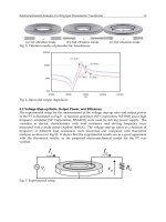
5.2 DNNO implementation (Contaminated Soil Treatment by Ozonation)
High oxidation process employing ozone is one of the most recent approaches in the
treatment of the contaminated soil with chemical compounds such as polyaromatic
hydrocarbons. The next simplified model (32) describes the ozonization of one contaminant
in the solid and gas phases in a semi-continuous reactor (Poznyak T., et. al. 2007).

(t)(t)xxGk(t)x
dt
d
(t)(t)xxk
t,
x
dt
d
(t)x
free_abs
max
Q
abs
t
Kx
dt
d

(t)x
free_abs
max
Q
abs
t
K(t)x
t,
xk(t)x
gas
W
in

C
gas
W
gas
V(t)x
dt
d
34
1
14
3413
22
23411
1
1
−
−=
=
⎟
⎠
⎞
⎜
⎝
⎛
−=
⎢
⎣
⎡
⎥
⎦

⎤
⎟
⎠
⎞
⎜
⎝
⎛
−
−−−
−
=
(32)
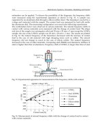
Here in (32)
η(t)(t)xy(t) +=
1
(see Figures 2 and 3 ) is the ozone concentration (mole/L) at
the output of the reactor assumed to be on-line measurable,
(t)x
2
(mole) is the ozone
amount absorbed by the soil, which is not reacting with the contaminant,
(t)x
3
(mole) is
the ozone amount absorbed by the soil and reacting with the contaminant, and
(t)x
4

(mole/g) is the current contaminant concentration,
in

C
is the ozone concentration at the
reactor input (mole/L),
free_abs
max
Q
is the maximum amount of ozone, which can be
absorbed by the soil,
Wgas is the gas flow (L/s) (established as a constant value), Vgas is
the volume of the gas phase.
(L).
Figure 2. Contaminated soil ozonation procedure in a semi-continuous batch reactor
Systems, Structure and Control

72
It is worth notice that the model is employed only as a data source; any structural
information (mathematical model) has been used in the projectional DNNO design.
The convex compact set
X
according to the physical system constrictions is given as:

⎪
⎪
⎪
⎭
⎪
⎪
⎪
⎬
⎫

⎪
⎪
⎪
⎩
⎪
⎪
⎪
⎨
⎧
≤≤
≤≤
≤≤
≤≤
(t)x(t)x
in
C
gas
V(t)x
free_abs
max
Q(t)x
(t)x(t)x
X:=
44
0
3
0
2
0
11

0
(33)
Projectional operator is defined as in (6), and the corresponding observer parameters are
defined by:

⎥
⎥
⎥
⎥
⎥
⎦
⎤
⎢
⎢
⎢
⎢
⎢
⎣
⎡
−
−
=
⎥
⎥
⎥
⎥
⎥
⎦
⎤
⎢

⎢
⎢
⎢
⎢
⎣
⎡
−
−
−
−
=
0.1
0.0001
0.01
0.01
K,
0.46000
02.2400
001.60
0002.6
A
(34)
Figures 4-7 represent the results of
3
x and
4
x estimation from the measurable output.
We have compared the projectional DNNO against a DNNO without projection operator, it
means, with and without considering physical restrictions in the DNNO structure.
Simulation have been realized in the presence of "quasi-white noise"

)t(
η

(amplitude ).
5
1060
−
×= and with the same initial conditions in both cases.



0 5 10 15 20 25
-0.5
0
0.5
1
1.5
2
2.5
3
x 10
-3
Ti me [ s]
mol e/ L
y Measurabl e Output

Figure 3. Measurable output (available information)