Systems, Structure and Control 2012 Part 6 doc

Integral Sliding Modes with Block Control of Multimachine Electric Power Systems

93
Thus, the trajectories of the last variables vector
r
z are asymptotically stable.
Step r-1. Proceeding in similar way as in previous step, the Lyapunov function
111
T
rrr−−−
=Vss
is proposed, then

() ()
11 11 1 1
() ,
T
rr rr r r
sigm t
ρ
−− −− − −
= ⎡−+⎤
⎣
⎦
Vs x s g x

. (41)
In the region
11rr
ε
−−

>s the equation (41) becomes

() ()
()
11 11 1 1
111 1
() ,
() ,
T
rr rr r r
rrr r
sign t
t
ρ
ρ
−− −− − −
−−− −
= ⎡−+⎤
⎣
⎦
⎡⎤
≤− +
⎣⎦
Vs x s g x
sxgx

. (42)
Moreover, under the condition
()
11 1

(, )
rr r
t
ρ
−− −
>xgz,
1r −
s will be decreasing until it
reaches the set
{
}
11rr
ε
−−
≤s in a finite time and it remains inside. The upper bound of this
reaching time can be calculated by using the comparison lemma (Khalil, 1996) as follows:
()
11 1
0
rr r
t
ε
−− −
≤−s .
Furthermore the equivalent control
1,1req−
x fulfills

11,1 1 11
(, )

rreqr rr
t
ε
−− − −−
=+ =sx gz γ

(43)
where
11rr
ε
−−
γ
is the error introduced by using the control law (29). To analyze the stability
of the r-1 block of the system (38), the Lyapunov function
111
1
2
T
rrr
−−−
=Vzz
is considered
and its time derivative is given by
()
()
1
11 11 1 11 1
1
2
1

11 1 11 1
1
() ,
() ,.
T
r
rr rr rrrr r
r
r
rr r r rr r
r
ksigmt
ksigmt
ρ
ε
ρ
ε
−
−− −− − −− −
−
−
−− − −− −
−
⎡
⎤
⎛⎞
=− + − +
⎜⎟
⎢
⎥

⎝⎠
⎣
⎦
⎡
⎤
⎛⎞
≤− + − +
⎜⎟
⎢
⎥
⎝⎠
⎣
⎦
s
Vz zEz x g z
s
zzz x gz


In the region
11rr
ε
−−
>s
, the derivative
1r −
V

becomes
()

2
1
111 1 1 1
1
2
11 1 1
,
r
rrr rrr r
r
rr r r r
ksignt
k
ρ
ε
−
−−− − − −
−
−− − −
⎡
⎤
⎛⎞
≤− + − +
⎜⎟
⎢
⎥
⎝⎠
⎣
⎦
⎡⎤

≤− + +
⎣⎦
s
Vzzz gz
zzzs



and considering (43), it can be rewritten as

2
111 1 11rrr rrrr
k
ε
−−− − −−
⎡
⎤≤− + +
⎣
⎦
Vzzzγ

. (44)
Suppose that
11rr
ε
−−
γ satisfies the following bound:
11 1 1 1 1 1
,,
rr r r r r r

R
εα βαβ
−− − − − − −
≤+ ∈γ z .
Then it is possible to present the equation (44) of the form
Systems, Structure and Control

94
()
2
111 1 111
1111 1
rrr rrrrr
rrrr rr
k
k
αβ
αβ
−−− − −−−
−−−− −
⎡
⎤
≤− + + +
⎣
⎦
⎡⎤
≤− − − −
⎣⎦
Vzzzz
zzz



which is negative in the region

11 1rrrr
δλ
−− −
>+zz
(45)
where
1
11
1
r
rr
k
δ
α
−
−−
=
−
and
1
1
11
r
r
rr
k

β
λ
α
−
−
−−
=
−
. Moreover
1r
δ
−
and
1r
λ
−
are positive for
11rr
k
α
−−
> . Thus the trajectories of the vector state enter ultimately in the region defined by
11 1rrrr
δλ
−− −
≤+zz.
Step i. The step r-1 can be generalized for the block i, with i=r-1, r-2, …, 1.
In the region
ii
ε

>s the derivative of the Lyapunov function
T
iii
=Vss, is calculated as

() ()
()
() ,
() , .
T
ii ii i i
iii i
sign t
t
ρ
ρ
= ⎡−+⎤
⎣
⎦
⎡⎤
≤− +
⎣⎦
Vs x s g x
sxgx

(46)
Again, under the condition
()
() ,
ii i

t
ρ
>x
g
z ,
i
s enter in the region
{
}
ii
ε
≤s in a finite time
given by
()
0
ii i
t
ε
≤−s .
The equivalent control
,1ieq
x satisfies

,1
(, )
iieqi ii
t
ε
=+ =sx gz γ


. (47)
Considering the function
1
2
T
iii
=Vzz inside the subspace
ii
ε
>s , it follows
()
2
1
2
1
() ,
i
iiiiiii i
i
ii i i i
ksignt
k
ρ
ε
+
+
⎡
⎤
⎛⎞
≤− + − +

⎜⎟
⎢
⎥
⎝⎠
⎣
⎦
⎡⎤
≤− + +
⎣⎦
s
Vzzz x gz
zzzs



and with (47),
i
V

becomes
2
1iii ii ii
k
ε
+
⎡
⎤≤− + +
⎣
⎦
Vzzzγ



Supposing that
ii
ε
γ fulfills
,,
ii i i i i i
R
εα βαβ
≤+ ∈γ z
then
()
1iiiiiii
k
αβ
+
⎡
⎤≤− − − −
⎣
⎦
Vz zz


which is negative in the region
Integral Sliding Modes with Block Control of Multimachine Electric Power Systems

95
1iii i
δλ

+
>+zz

where
1
i
ii
k
δ
α
=
−
and
i
i
ii
k
β
λ
α
=
−
, which are positive for
ii
k
α
> . Therefore a solution for
i
z
is ultimately bounded by

1iii i
δλ
+
≤+zz .
Then with the bound
,1,2, ,1
ii i i i
ir
εα β
≤+= −γ z
the convergence region is defined by:
11 11
22122
11211
:
:
:.
rrrrr
rrrrr
h
h
h
δλ
δλ
δλ
−− −−
−−−−−
>+=
>+=
>+=

zz
zz
zz


4. PES control design
Since the subsystem (10) has the NBC form, the ISM technique will be applied to design a
robust controller for EPS. First, the rotor speed stability will be achieved. Secondly, the
terminal voltage generator controller is outlined. Then, a switching logic is proposed to
coordinate the operation of both controllers. Finally, an EPS observer is introduced.
4.1 Integral Sliding Mode Speed Stabilizer (ISMSS)
To achieve the first control objective, that is, the rotor speed stability enhancement, define
the control error as (Huerta-Avila et al., 2007a, Huerta-Avila et al., 2007b)

22iib
zx
ω
=−. (48)
Taking the time derivative of (48) along the trajectories of (10) yields

232
(, ) (, ) (, , )
i iii iii i iiimi
zf q xg T
ω
=− +xv xv xv

(49)
where
()

12
T
iii
=xxx, () 0, 0
i
qt t>∀>.
Redefine the virtual control,
3i
x
in (49) as

33,03,1ii i
x
xx=+. (50)
The desired dynamics for
2i
z is chosen of the form

223 3,12
(, ) (, , ), 0
i ii i iii i iiimi i
zkzzq xg Tk=− + + + >xv xv

(51)
These dynamics can be obtained by choosing
3,0i
x
as
Systems, Structure and Control

96

() ()
1
3,0 2 3
,,
iiiiiiiiii
x
qfkzz
ω
−
=−⎡⎤⎡ +−⎤
⎣
⎦⎣ ⎦
xv xv
(52)
where
3i
z is a new variable. To design the second part of (50),
3,1i
x
, define a pseudo-sliding
variable
2i
s
as
22 2ii i
sz
σ
=+

with the integral variable
2i
σ
. Using (49)-(51), it follows

,
2023 3,12 2
(, ) (,)
iiiiiiiiiiimii
qxskzz g T
σ
++=− + +xv vx

(53)
Choosing
2223 2 2
,(0)(0)
iiii i i
kz z z
σσ
=− =−


the equation (53) becomes
,
22 3,1
(, )(,)
iiiimiiiii
qxsg T+= vxvx


.
Select
3,1i
x
of the form

3,1 2 2 2
(/), 0
ii iii
xsigms
ρ
ε
ρ
=− > . (54)
Then, the sliding variable
3ii
s
z
ω
= is defined from (50), (52) and (54) of the form

()
302 2 2
(, ) (,) /
iiiiiiiiiii ii
sf q xkz sigms
ωω
ρ
ε
=+ ++xv xv

. (55)
Thus, straightforward algebra reveals

(, ) (, )
i siii siiifi
s
fbv
ω
=+xv xv

(56)
where
()
si
f
⋅ is a continuous function and
4
() ()
s
iii
bqb⋅= ⋅ .
Considering (56), under the condition
1
(, ) (, )
g
isiiisiii
kb f
−
> xv xv
the proposed discontinuous control law

(), 0
fi gi i gi
vksigns k
ω
=− > (57)
ensures the convergence of the state to the manifold
3
0
ii
sz
ω
== (55) in a finite time (Utkin
et al., 1999). The sliding mode motion on this manifold is governed by the reduced order
system

12
,
2022 2 2
,
22 2 2
,
(/)
(/)
(,)
(,)
ii
iiii iiiiimi
ii iiiiimi
xz

zkz sigms
sigm s
g
T
sgT
ρε
ρε
=
=− − +
−+
=
v
v
x
x



(58)
Integral Sliding Modes with Block Control of Multimachine Electric Power Systems

97

()
2222
,
iiiiii
=+xAxfxv



(59)
Now, choosing
i
ε
be sufficiently small and under the condition
()
22
,,
iiiimi
gT
ρ
> xv

a quasi sliding mode motion is enforced in a small
i
ε
-vicinity of
2
0
i
s =
. Thus, if
0
i
ε
→

then the perturbation term
()
2

,,
ii imi
g
Txv in (59) is rejected, and the linearized mechanical
dynamics can be represented as

12
202
ii
iii
xz
zkz
=
=−


(60)
with the desired eigenvalue
0i
k− .
The equation (59) represents the rotor flux internal dynamics. The matrix
2i
A is Hurwitz
and the nonvanishing perturbation
()
2
,
iii
fxV


is a continuous function. Therefore there
exists an admissible region where a solution
2
()
i
tx of (60) is ultimately bounded (Khalil,
1996). Moreover, the control error
2i
z (48) tends exponentially to zero, and the angle
1i
x

tends to a constant steady state,
s
si
δ
.
Remark: Since the initial conditions of the EPS are availabe, it is possible to apply the integral
sliding modes technique.
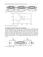
4.2 Sliding Mode Voltage Regulator

In this subsection, the voltage regulation problem is studied. The terminal voltage,
g
i
v , is
defined as

222
g
idiqi

vvv=+
. (61)
Using (8),
di
v
and
qi
v are calculated of the form

1
[()]
di
iiziizii
qi
v
v
−
⎡⎤
==− +
⎢⎥
⎣⎦
vHAifx
. (62)
Then, the dynamics for terminal voltage,
g
i
v can be obtained from (61), (62), (6), and (7) as
(Loukianov, et al., 2006)

(,) (,, )

g
iviii vifiviiimi
vf bvg T=++xi xi

(63)
where
(,)
vi i i
f xi is the nominal part of the voltage dynamics and the perturbation term
(,, )
vi i i mi
g
Txi
contains parameter variations and external disturbances,
24vi i i
bhb= ,
(), 0
vi
bt t∀≥ . For the details see Appendix.
Defining the voltage control error
Systems, Structure and Control

98
vi gi refi
evv=−
and the control input
f
i
v

,0 ,1
f
ifi fi
vv v=+
(64)
we have

,0 ,1
(,) (,, )
v i vi i i vi fi vi fi vi i i mi
e f bv bv g T=+++xi xi

(65)
where
refi
v is the constant reference voltage. To design a robust controller we use the
integral sliding mode approach (Utkin et al., 1999). In order to reject the perturbation term
(,, )
vi i i mi
g
Txi
in (65) a sliding variable
vi
s
R∈ is formulated as

vi vi vi
se
σ
=+ (66)

with the integral variable
vi
R
σ
∈ . Then from (65) and (66) it follows

,0 ,1
(,) (,, )
v i vi i i vi fi vi fi vi i i mi vi
sf bv bv g T
σ
=+++ +xi xi

(67)
Choosing
,0
(,) , (0) (0)
vi vi i i vi fi vi vi
fbv e
σσ
=− − =−xi


results in

,1
(,, )
v i vi fi vi i i mi
s
bv g T=+xi


(68)
Select
,1
f
i
v in (68) as

,1 2 2
(), 0
fi i vi i
vsigns
ρρ
=− > . (69)
From (68), under the condition
1
2
(,, )
iviviiimi
bg T
ρ
−
> xi a sliding mode is enforced on the
manifold 0
vi
s = (66) from the initial time instant 0t = . The equivalent control
1
,1
(,, )
f

ieq vi vi i i mi
vbgT
−
=− xi
calculated as a solution of
0
vi
s =

(67), compensates exactly the perturbation term
(,, )
vi i i mi
g
Txi in (63) (Utkin et al., 1999), and the sliding mode motion is described by the
unperturbed system

,0
(,)
vi vi i i vi fi
ef bv=+xi

. (70)
Now, it is necessary to achieve the terminal voltage regulation, i. e. the control input
,0
f
i
v in
(70) is selected of the form

()

,0
f
igvi
vksigne=−
(71)
From (70) and (71), we have
Integral Sliding Modes with Block Control of Multimachine Electric Power Systems

99

()
(,)
vi vi i i g vi vi
ef kbsigne=−xi

. (72)
Then, under the condition

1
(,)
g
vi vi i i
kbf
−
> xi (73)
the terminal voltage control error
vi
e tends to zero in a finite time (Utkin et al., 1999).
4.3 Control logic

There are two control objectives: the rotor speed stabilization and the terminal voltage
regulation for each generator in the EPS. However, only one control input is available, the
excitation voltage
f
i
v . Then, the following control logic is proposed:

()
13
223
(),
,
(),
gi i i i
ivii
fi i
g
vi i vi i i i vi i
k sign s if s
if
v
ksigne signs if s if
ωω
ω
β
βββ
β
ρββββ
⎧
−>

⎧
>
⎪⎪
==
⎨⎨
−− ≤ ≤
⎪
⎪
⎩
⎩
(74)
with
21ii
ββ
<
. Basically, a hierarchical control action through the proposed logic (74) is
presented. First, the mechanical dynamics is stabilized by means of the ISMSS, yielding the
stabilization of the speed switching manifold
i
s
ω
. When
i
s
ω
reaches to a region defined by
1i
β
, the control resources are dedicated to stabilize the terminal voltage error
vi

β
. After the
convergence of
vi
β
such that
3vi i
ββ
≤ , the control logic reduces the
i
s
ω
boundary layer
width from
1i
β
to
2i
β
. Thus, the controller maintains the value of
i
s
ω
within desired
accuracy
2ii
s
ω
β
≤ and

3vi i
e
β
≤ . Figure 1 shows the schematic diagram of the proposed
controller.


Figure 1. Proposed controller schematic diagram
Systems, Structure and Control

100
4.4 EPS observer
Since the control scheme (74) needs the values of the rotor fluxes, it is neccesary to design a
observer for the EPS. Assume that the power angle,
1i
x
, rotor speed,
2i
x
and stator currents
di
i and
qi
i can be measured.
The rotor fluxes
,,
345iii
x
xx and
6i

x
can be estimated by means of the following observer:

3
13 25 3
4
14 26 3
4
13 25 3
5
14 26 3
6
ˆ
ˆˆ
ˆˆ
ˆ
0
ˆˆ
0
ˆ
ˆˆ
0
ˆ
i
ii i i idi
i
ii i i iqi
i
f
i

ii i i idi
i
ii i i iqi
i
x
bx bx bi
b
cx c x ci
x
v
dx d x di
x
rx rx ri
x
⎡⎤
++
⎡⎤
⎡
⎤
⎢⎥
⎢⎥
⎢
⎥
++
⎢⎥
⎢⎥
⎢
⎥
=+
⎢⎥

⎢⎥
⎢
⎥
++
⎢⎥
⎢⎥
⎢
⎥
⎢⎥
++
⎢
⎥
⎢⎥
⎣
⎦
⎣⎦
⎢⎥
⎣⎦




(75)
where
[]
3456
ˆˆˆˆˆ
,,,
T
iiiii

xxxx=x are the estimate of the rotor fluxes. The convergence of the
observer (75) can be analyzed by the error dynamics obtained from (75) and (6), given by the
linear system:

0ii
=eA

(76)
with
[
]
36
,,
ii i
e e=e … , , 3, ,6
ˆ
ji ji ji
jexx ==− ,
12
12
0
12
42
00
00
00
00
ii
ii
i

ii
ii
bb
cc
dd
rr
⎡
⎤
⎢
⎥
⎢
⎥
=
⎢
⎥
⎢
⎥
⎢
⎥
⎣
⎦
A
.
The eigenvalues of the matrix
0i
A
calculated as
()
()
22

1,2 1 2 1 2 1 2 2 1
22
3,4 1 2 1 2 1 2 2 1
11
24,
22
11
24
22
iii iiiiii
iii iiiiii
pcr crcrcr
pbd bdbdbd
=+± +− +
=+± +− +

are real and negative. Therefore, the solution of the subsystem (76) is exponentially stable.
The resulting estimates rotor fluxes are employed in the control logic (74) instead of the real
variables.
5. Simulations results
The proposed control algorithm was tested on the equivalent model of the WSCC, (Western
System Coordinating Council, Nine buses, three generators, three loads), fig. 2, (Anderson &
Fouad, 1994). The parameters of the generators and network used in the simulation were
taken from (Anderson & Fouad, 1994) (see Appendix).
Figures 3-8 depict results under four different events:
a. at t = 1 s, experienced a pulse 0.5 p.u. for 1 s in the generator 2,
b. at t = 4 s until t = 4.15 s, a three-phase short circuit is simulated in the terminals of
generator 1,
c. at t = 10 s, a three-phase short circuit during 150 ms is applied in the line 5-7 (see fig. 2);
the fault is cleared by opening the line, and

Integral Sliding Modes with Block Control of Multimachine Electric Power Systems

101
d. at t=15 s, it was introduced a parametric variations, by incrementing up to 25% the
parameters
mi
L in the generators.
Figures 3 and 5 show the relative angles and speed response of the close-loop system,
respectively with a type I excitation system with PSS (Anderson & Fouad, 1994, EPRI, 1977).
Figure 8 show the proposed observer converge in spite of perturbations.
Figures 4-7 reveal some important aspects:
1. The state variables fastly reach a steady state condition after small and large
disturbances, showing the robust stability of the closed-loop system.
2. The controller is able to improve both, the power system stabilization and the post-fault
terminal voltage regulation.
Comparing the transient speed response of the generators in case of ISMSS /SMVR and
AVR/ PSS controllers shown in Figures 6 and 5 respectively, we have some important
observations:
1. The traditional AVR/PSS stabilizes the system. However, the transient response of the
classical controller is more oscillatory than the response given by the proposed
nonlinear ISMSS /SMVR one since the latter adds significantly better damping in the
power oscillations. It is possible to observe that the overshoot and settling time are
reduced as well.
2. The performance of the ISMSS /SMVR is robust under different operating conditions.
Figures 4 and 6 show clearly that the robustness of the controller under generators
parameters variations and changes on the network configuration, such as disconnection
of lines and incrementing and /or decrementing of loads. Thus the performance of the
proposed ISMSS /SMVR controller tends to be unaffected.
3. Since the ISMSS /SMVR adds additional damping, the transient response controller is
better compared to other ones (see for instance (Ahmed at al., 1996)). With the ISMSS

/SMVR, the settling time is lesser and the overshot is shorter than the shown by the
suboptimal robust controller presented in (Ahmed at al., 1996).



Figure 2. WSCC diagram
Systems, Structure and Control

102

Figure 3. Relative angles response with classical control


Figure 4. Relative angles response with the proposed controller


Figure 5. Speed of the three generators response with classical control
Integral Sliding Modes with Block Control of Multimachine Electric Power Systems

103

Figure 6. Speed of the three generators response with the proposed controller

Figure 7. Terminal voltage of the three generators response with the proposed controller

Figure 8. Field flux of the three generators response

Systems, Structure and Control

104

6. Conclusions
The ISM with block control technique as a novel nonlinear control technique for the class of
nonlinear systems presented in the NBC form was presented. The control methodology was
explained step-by-step, and the stability conditions were found for each step. The ISM
technique is robust under unknown but bounded matched and/or unmatched
perturbations.
Then, in order to test the effectiveness of the ISM technique, a controller for EPS was
designed. A plant model used for control is fully detailed nonlinear, and this model takes
into account all interactions in power system between the electrical and mechanical
dynamics and load constraints. With the proposed control scheme, the only local
information is required. The stability analysis of the closed-loop EPS controller, including an
observer was carried out. The designed ISMSS/SMVR was tested through simulation under
the most important perturbations in the EPS:
1. Variation of the mechanical torque.
2. Large fault (a 150 ms short circuit).
3. Loads variations.
4. Generator parameter variations.
The simulation results show that the sliding mode controller with the proposed logic is able
to achieve the mechanical dynamics and the generator terminal voltages robust stability
under small and large disturbances.
The proposed performance of the nonlinear ISMSS/ SMVR control system (74) is
independent from the operating point of the system. It is important to note that the
proposed nonlinear control scheme ensures cancellation of the interactions between the
subsystems provided an additional damping with respect to classical controllers.
7. References
Abidi, K. & Šabanovic, A., (2007). Sliding-mode control for high-precision motion of a
piezostage, IEEE Trans. on Industrial Electronics, vol. 54, no. 1, pp. 629-637, 2007.
Adhami-Mirhosseini, A. & Yazdanpanah, M. J., (2005). Robust Tracking of perturbed
systems by nested sliding mode control. Proc. of ICCA2005, Budapest, Hungary,
June 2005.

Aggoune, M. E., Boudjeman, F., Bensenouci, A., Hellal, A., Elmesai, M.R., & Vadari, S.V.,
(1994). Design of Variable Structure Voltage Regulator Using Pole Assignment
Technique, IEEE Transaction on Automatic Control, Vol. 39, No. 10, October 1994.
Ahmed, S. S., Chen, L. and Petroianu, A., (1996), Design of Suboptimal H∞ Excitation
Controller, IEEE Trans. on Power Systems, Vol. 11, No. 1, February, 1996.
Akhkrif, O., Okou, F., Dessaint, L., & Champagne, R., (1999). Application of Multivariable
Feedback Linearization Scheme for Rotor Angle Stability and Voltage Regulation of
Power System, IEEE Trans. Power Syst., Vol.14, No.2, pp.620-628, 1999.
Anderson, P. M., & Fouad, A., (1994). Power System Control and Stability, IEEE Press New
York, 1994.
Bandal, V., Bandyopadhyay, B., & Kulkarni, A. M., (2005). Decentralized Sliding Mode
Control Technique Based Power System Stabilizer (PSS) for Multimachine Power
System, Proc. Conference on Control Applications, Toronto, Canada, August, 2005.
Integral Sliding Modes with Block Control of Multimachine Electric Power Systems

105
Dash, P., Sahoo, N., Elangovan, S., & Liew, A., (1996). Sliding Mode Control of a Static
Controller for Synchronous Generator Stabilization, Electrical Power & Energy
Systems, Vol. 18, pp. 55-64, 1996.
DeMello, F. P. & Concordia, C., (1969). Concepts of Synchronous Machine Stability as
Affected by Excitation Control, IEEE Trans., PAS-88, Apr. 1969, 316-329.
Djukanovic, M., Khammash, M. and Vittal, V. (1998a), Application of the structured value
theory for robust stability and control analysis in multimachine power systems, Part I:
Framework development, IEEE, Trans. on Power Systems, Vol. 13, No. 4, November
1998.
Djukanovic, M., Khammash, M. and Vittal, V. (1998b), Application of the structured value
theory for robust stability and control analysis in multimachine power systems, Part II:
Numerical simulations and results, IEEE, Trans. on Power Systems, Vol. 13, No. 4,
November 1998.
EPRI report, (1977). Power System Dynamic Analysis Phase I, EPRI EL-484, Project 670-1, July

1977
Huerta-Avila, H. (2005). Control no lineal robusto de sistemas eléctricos de gran escala por modos
deslizante, M. Sc. Thesis, Scientific advisors: A. G. Loukianov and J. M. Cañedo,
CINVESTAV, Unidad Guadalajara, México, September 2005.
Huerta-Avila, H., Loukianov, A. G., & Cañedo, J. M. (2007a). Nested Integral Sliding Mode
Control of Multimachine Power Systems, Proc. of SSSC07, Iguazu, Brazil, October
2007.
Huerta-Avila, H., Loukianov, A. G., & Cañedo, J. M. (2007b). Nested Integral Sliding Mode
Control of Large-Scale Power Systems, Proc. of CDC07, New Orleans, EUA,
December 2007.
Jung, K., Kim, K., Yoon, T. & Jang, G. (2005). Decentralized Control for Multimachine Power
Systems with Nonlinear Interconnections and Disturbances, International Journal of
Control, Automation, and Systems, Vol 3, No. 2 (especial edition), pp. 270-277, June
2005.
Khalil, H. K., (1996). Nonlinear systems, Prentice Hall, Inc. Simon and Schuster, New Jersey,
1996.
King, C. A., Chapman, J. W. & Ilic, M. D., (1994). Feedback linearizing excitation control on a full
scale power system model, IEEE Trans. Power Systems, 9, 1102-1109, 1994.
Kshatriya, N., Annakkage, U. D., Gole, A. M. & Fernando, I. T., (2005). Improving the
Accuracy of Normal Forma Analysis, IEEE Trans. on Power Systems, Vol. 20, No. 1,
February 2005.
Liu, S., Messina, A. R., & Vittal, V., (2006). A Normal Form Analysis Approach to Siting
Power System Stabilizers (PSSs) and Assesing Power System Nonlinear Behavior,
IEEE Trans. on Power Systems, Vol. 21, No. 4, November 2006.
Loukianov, A.G., (1998), Nonlinear Block Control with Sliding Mode, Automation and Remote
Control, Vol.59, No.7, pp. 916-933, 1998.
Loukianov, A. G., Cañedo, J. M., Utkin, V. I. & Cabrera-Vázquez, J., (2004). Discontinuos
Controller for Power Systems: Sliding-Mode Block Control Approach, Trans. on
Industrial Electronics, Vol., No. 51, No. 2, April 2004, pp. 340-353.
Loukianov, A, G., Cañedo, J. M., & Huerta, H., (2006) Decentralized Sliding Mode Block Control

of Power Systems, Proc. of PES General meeting 2006, Montreal, Quebec, Canada,
June, 2006.
Systems, Structure and Control

106
Machowsky, J., Robak, S., Bialek, J. W., Bumby, J. R., & Abi-Samra, N., (2000). Decentralized
Stability-Enhancing Control of Synchronous Generator, IEEE Transactions on Power
Systems, Vol. 15, No. 4, November 2000.
Mohagheghi, S., Valle, Y., Venayagamoorthy, G. K., & Harley, R. G., (2007). A proportional-
integrator type adaptive critic design-based neurocontroller for a static compensator in a
multimachine power system, IEEE, Trans. On Industrial Electronics, Vol. 54, No. 1,
February, 2007.
Topalov, A.V., Cascella, G.L., Giordano, V., Cupertino, F., & Kaynak, O., (2007). Sliding
mode neuro-adaptive control of electric drives, IEEE Trans. on Industrial Electronics,
vol. 54, no. 1, pp. 671-679, 2007.
Utkin, V. I., Guldner, J., & Shi, J., (1999). Sliding Mode Control in Electromechanical
Systems, Taylor & Francis, London, 1999.
Venayagamoorthy, G. K., Harley, R. G., & Wunsch, D. C., (2003). Dual Heuristic
Programming Excitation Neruocontrol for Generators in a Multimachine Power
System, IEEE Trans on Industry Applications, Vol. 39, No. 2, March/April 2003.
Wang, Y., Hill, D. J., & Guo, G., (1998). Robust Decentralized Control for Multimachine
Power Systems, IEEE Trans on Circuits and Systems-I:Fundamental Theory and
Applications, Vol. 45, No. 3, March 1998, pp 271-279
Wu, B. & Malik, P., (2006). Multivariable Adaptive Control of Synchronous Machines in a
Multimachine Power System, IEEE Trans on Power Systems, Vol. 21, No. 4,
November 2006.
Xie, W., (2007). Sliding-mode-observer-based adaptive control for servo actuator with
friction, IEEE Trans. on Industrial Electronics, vol. 54, no. 3, pp. 1517-1527, 2007.
Yildiz, Y., Šabanovic, A., & Abidi, K., (2007). Sliding mode neuro-controller for uncertain
systems, IEEE Trans. on Industrial Electronics, vol. 54, no. 3, pp. 1676-1685, 2007

Yousef, A. M. & Mohamed, M. A., (2004). Multimachine Power System Stabilizer Based on
Efficient Two-Layered Fuzzy Logic Controller, Transactions on Engineering and
Technology V3, December 2004, pp.137-140.
8. Appendix
8.1 Matrices used in generator model (1)
()
11 12
66
21 22
, ,
00
() ,
0
f g kd kq s s
diag R R R R R R R
I
ω
ω
×
⎡⎤
⎢⎥
⎢⎥
⎢⎥
⎣⎦
⎡⎤
⎡⎤
=
⎢⎥
⎣⎦
⎣⎦

=−− =∈
LL
L
LL
RW

()
11 12
21 22
00
0
0
00
0
00
0
00
00 0
00 0
0
,
0
fmd
md
mq
gmq
md
md kd
mq
mq kq

md md d
mq mq q
LL
L
L
LL
L
LL
L
LL
LL L
LL L
I
ω
ω
ω
⎡
⎤
−
⎛⎞
⎛⎞
⎢
⎥
⎜⎟
⎜⎟
−
⎢
⎥
⎜⎟
⎜⎟

⎢
⎥
⎜⎟
⎜⎟
−
⎡⎤
⎡⎤
⎢
⎥
⎜⎟
⎜⎟
=
⎢⎥
⎢⎥
⎜⎟
⎜⎟
⎢
⎥
−
⎝⎠
⎣⎦
⎣⎦
⎝⎠
⎢
⎥
⎢
⎥
−
⎛⎞⎛⎞
⎢

⎥
⎜⎟⎜⎟
⎜⎟⎜⎟
−
⎢
⎥
⎝⎠⎝⎠
⎣
⎦
−
=
LL
LL
.
Integral Sliding Modes with Block Control of Multimachine Electric Power Systems

107
d
L
and
q
L
are the direct-axis and quadrature-axis self-inductances,
f
L
is the field self-
inductance,
g
L
,

kd
L
and
kq
L
are the damper windings self-inductances,
md
L
and
mq
L
are the
direct-axis and quadrature-axis magnetizing inductances
4
21 22
0
⎡⎤
=
⎢⎥
⎣⎦
I
T
TT
,
11111
21 2 222111 12 222111
1111
22 2 22 21 11 12 22
[],
[],

−−−−−
−−−−
=− −
=− −
T I LLL L LLL
TILLLLL
,
2
I and
4
I are identity matrices of
dimension 2 and 4, respectively.
8.2 Generators parameters
12 3 4 5
123
000
'' ''
'' ''
, , , , '' '' ,
1'' '' ''
1, , ,
''(')''
qi ai qi ai
di ai di ai
ii i i iqidi
fi gi kdi kqi
di ai mdi di ai mdi di ai
imdii i
d i kdi fi d i di ai kdi d i di ai
Ll Ll

Ll Ll
aa a a aLL
lll l
Ll L Ll LLl
bLb b b
ll L l l L l
τττ
−−
−−
==−= =−=−
⎛⎞
−− −
=− + = =−
⎜⎟
⎜⎟
−−
⎝⎠
()
4
1231
0g 0 0 0
23 1 2
000g
,
'' '' ''
1'
1, , ,,
''''''
'
'

1' 1
,,,
'' '' ''
is
qi ai q a mq mqi qi ai
di ai
imqiiii
qi kqi i q qi qi ai di fi
qakq
qi ai
di ai
ii i i
di di qi i
Ll LlL LLl
L
l
cLccd
ll L l l
Lll
Ll
Ll
dd r r
l
ω
ττττ
τττ τ
=
⎛⎞ ⎛⎞
−− −
−

=− + = =− =
⎜⎟ ⎜⎟
⎜⎟ ⎜⎟
−
−
⎝⎠ ⎝⎠
−
−
=− =− = =−
31
00
'
,,,
'' '' ''
qi ai
s
ii
qi qi di
Ll
rh
L
ω
τ
−
=− =−


()
2 4
00

53
0
''
1''1''' 1
1,,
'' ' '' '' '' ''
''
'' '' 1
,
'' '' ' '
qi ai
di ai di ai di ai di ai
imdi i
di d i f i kdi fi di d i di kdi fi di gi
qi ai
mdi diai diai
ii
di kqi d i d i d i ai kdi fi
Ll
LlLl L lLl
hL h
LlllLLllLl
Ll
LLlLl
hh
Ll L L ll l
ττ
τ
⎛⎞
−

−− −−
=− + + =−
⎜⎟
⎜⎟
⎝⎠
−
−−
=− = −
−
()
68
0
17
00
4
''
'' ( '' )
,, ,
'' '' '' '' ''
'
''''' ''
,,
'' '' '' ' ' '' ' ''
1
'
qi
di ai s di ai
ii
di d i di kdi di di fi
di ai

s sai mdi diai diai diai diai
ii
di di di d i fi fi di ai di d i di kdi
i
L
Ll Ll
hh
LLl L Ll
Ll
r L LlLlLl Ll
kh
LLLllLlLLl
k
L
ω
τ
ωω
ττ
−−
==
−
−−− −
=− =− − −
−
=−
()
2
00
56
3

0
'' ' '' '' ''
1
,,
' '' ' '' '' ''
'
''
1''
,,
'' '' ''
'' '
'' '' '
qi ai qi ai mqi qi ai qi ai q i ai
i
qi gi fi qi q i gi qi q i qi k di
qi ai kqi
qi ai
di
ii
qi qi kdi q i
mqi qi ai q
sai
i
qi qi q i gi
k
LlLl L LlLl Ll
k
ll L lL Ll
Lll
Ll

L
k
LLl L
LLlL
r
k
LL l
ττ
ω
τ
−− − − −
=−
−
−
=− =
−
=− −
()
0
7
00
'' ''
1
',
'''' ''
'' '''
11
1.
'' ' '' '' ''
iai qiai qiai

qi ai
gi qi ai qi q i qi kdi
qi ai qi ai qi ai qi ai
imqi
qi q i gi kqi gi qi q i qi k di gi
lL l L l
Ll
lLlL Ll
LlLl LlLl
kL
LlllLLll
τ
ττ
−− −
−−
−
⎛⎞
−− −−
=− + +
⎜⎟
⎜⎟
⎝⎠




Systems, Structure and Control

108
Generator 1 2 3

MVA 247.5 192.0 128.0
kV 16.5 18.0 13.8
P.F. 1.0 0.85 0.85
Type Hydro Steam Steam
Speed 180 r/min 3600 r/min 3600 r/min
X
d
0.1460 0.8958 1.3125
X
q
0.0969 0.8645 1.2587
X
d
’ 0.0608 0.1198 0.1813
X
q
’ 0.0969 0.1969 0.2500
τ
d0
’ 8.9600 6.0000 5.8900
τ
q0
’ 0.0000 0.5350 0.6000
X
d
’’ 0.0400 0.0600 0.0800
X
q
’’ 0.0400 0.0600 0.0800
τ

d0
’’ 0.2000 0.3000 0.4000
τ
q0
’’ 0.2000 0.3000 0.4000
X
l
0.0336 0.0521 0.0742
r
a
0.0000 0.0000 0.0000
H 23.6400 6.4000 3.0100
Table 1. Parameters of generator model (6)-(7)
Gen. 1 Gen. 2 Gen. 3 Gen. 1 Gen. 2 Gen. 3
a
1
0.1003 0.1644 0.0945 e
3
-5.000 -4.0 -2.5
a
2
1.13 1.1787 0.9458 h
1
-1256 -9424 -4712
a
3
0.0403 0.0119 0.0203 h
2
273.4 863.6 141.3
a

4
1.2552 1.0145 1.0239 h
3
0.5 -6.6 3.2
a
5
0.020 0.01 0.010 h
4
-31 -50.2 -16.4
b
1
-0.017 -0.0251 -0.0114 h
5
18.8 97.1 29.7
b
2
0.522 2.4483 1.8567 h
6
-0.1 -0.3 -0.3
b
3
-0.5075 -2.4185 -1.8659 h
7
-4.2 -25.4 -12.8
b
4
376.991 376.991 376.991 h
8
0.1 1.3 0.9
c

1
-0.07 -0.022 -0.0472 k
1
-1885 -7539 -5385
c
2
0.6453 10.6390 11.4979 k
2
1.7 11.8 6.4
c
3
-0.5348 -10.611 -11.4581 k
3
5.1 6.9 34.5
d
1
0.1360 -0.2257 0.2267 k
4
31.5 8.37 39.9
d
2
-3.79 -3.0659 -2.2838 k
5
0.5 3.3 0.7
d
3
-3.33 -3.333 -2.5 k
6
-5.7 -23.6 -13.5
e

1
0.2665 0.5792 0.4395 k
7
-0.1 -0.8 -1.1
e
2
-0.7899 -3.2871 -2.1290
Table 2. Generators parameters
Integral Sliding Modes with Block Control of Multimachine Electric Power Systems

109
Gen. 1 Gen. 2 Gen. 3 Gen. 1 Gen. 2 Gen. 3
a
1
0.2175 0.0916 0.03 e
3
-5.000 -4.0 -2.5
a
2
1.1324 1.1787 0.9458 h
1
-1256 -9424 -4712
a
3
0.0403 0.0119 0.0203 h
2
126.1 1549 233.1
a
4
1.2552 1.0145 1.0239 h

3
5 -6.8 3.2
a
5
0.020 0.010 0.010 h
4
-14.5 -100.3 -25.8
b
1
-0.003 -0.005 -0.0023 h
5
19 108.3 28.4
b
2
0.1044 0.4897 0.3713 h
6
-0.1 -0.3 -0.3
b
3
-0.0601 -0.0844 -0.0358 h
7
-3.2 -25.4 -12.8
b
4
376.991 376.991 376.991 h
8
1 1.3 0.9
c
1
-0.07 -0.022 -0.0472 k

1
-1885 -7539 -5385
c
2
0.6453 10.6390 11.4979 k
2
1.7 11.8 6.4
c
3
-0.5348 -10.611 -11.4581 k
3
5.1 69.2 34.5
d
1
0.1360 -0.2257 0.2267 k
4
31.5 83.7 39.9
d
2
-8.2182 -1.7090 -1.3842 k
5
1.1 1.8 0.4
d
3
-5.0 -3.333 -2.5 k
6
-5.7 -23.6 -13.5
e
1
0.2665 0.5792 0.4395 k

7
-0.1 -0.8 -1.1
e
2
-0.7899 -3.2871 -2.1290
Table 3. Perturbed generators parameters
Generator 1 Generator 2 Generator 3
k
gi
0.02 0.02 0.03
k
0i
7.5 5 6
ρ
2i
8 10 9
e
1
0.9 0.8 1.2
e
2
0.01 0.03 0.02
e
3
0.001 0.002 0.001
Table 4. Controllers parameters
Systems, Structure and Control

110
8.3 Functions used in controllers design

() ()()()()
()
()( )
()
()
1 2 24 442
1
213 25 3 3 13 25 31
1
214 26 32
1
4
34
1
,,,,,, ,
1
,
(,, ) (,)
viii diii iii qiii iii vi ii ii i
i
iiiiiidi iii ii ii
iii
iiiiiii
i
i
iiimi iii i i
fv v bhbkbx
k
hbx bx bi hdx dx di
xcx cx ci

h
h
fTqxx
ω
ϕϕ
ϕ
⎛⎞
=+ =+
⎜⎟
⎝⎠
+++ ++ +
=− ⎛⎞
+++
⎜⎟
⎜
−
⎝⎠
xi xi xi xi xi
xi
xi xi
()
()
()
()
()( )
()
214 26 32
5
36
24 3 14 26 32

242132531 33
1
52 13 2
,
(,, ) (,)
1
,(,,)(,)
iiiiiii
i
iiimi iii i i
ii iii ii ii
iii i iiiiiii iiimi iiiii
i
iiiii
xrx rx ri
h
fTqxx
kx k rx rx ri
kxbx bx bi f T q xx
k
kxdx d
ω
ω
ϕ
⎡
⎤
⎢
⎥
⎛⎞
+++

⎢
⎥
+
⎜⎟
⎢
⎥
⎟⎜ ⎟
−
⎢
⎥
⎝⎠
⎣
⎦
++++
=− + + + −
++
xi xi
xi xi xi

()( )
()
()
531 35
672262278
,
(,, ) (,)
, .
iii iiimi iiiii
vi i i i di i i qi i qi i i di i i qi i fi vi
xdi f T q xx

dd d dd
ghihxixikxixkihvf
dt dt dt dt dt
ω
⎡⎤
⎢⎥
⎢⎥
⎢⎥
++ −
⎢⎥
⎣⎦
⎛⎞⎛⎞
=+ ++ ++++Δ
⎜⎟⎜⎟
⎝⎠⎝⎠
xi xi
xi



5
Stability Analysis of Polynomials
with Polynomic Uncertainty
Petr Hušek
Dept. of Control Engineering, Faculty of Electrical Engineering, Czech Technical
University in Prague
Czech Republic
1. Introduction
When dealing with systems with parameter uncertainty most attention is paid to robustness
analysis of linear time-invariant systems. In literature the most often investigated topic of

analysis of linear time-invariant systems with parametric uncertainty is the problem of
stability analysis of polynomials whose coefficients depend on uncertain parameters. The
aim is to verify that all roots of such a polynomial are located in some prescribed set in
complex plane or to find a bound within that uncertain parameters can vary from nominal
ones preserving stability. The former problem is studied in this contribution.
The formulations of basic robustness problems and their first solutions for special cases are
very old. For example, in the work (Neimark, 1949) some effective techniques for small
number of parameters are presented. A powerful result concerning the stability analysis of
polynomials with multilinear dependency of its coefficients is given in the book (Zadeh &
Desoer, 1963). Also in Siljak’s book (Siljak, 1969) special classes of robust stability analysis
problems with parametric uncertainty are studied. Nevertheless, the starting point of an
intensive interest in this area was the celebrated Kharitonov theorem (Kharitonov, 1978)
dealing with interval polynomials. This elegant theorem with surprisingly simple result is
considered as the biggest achievement in control theory in last century. When analysing
stability of a polynomial with some dependency of its coefficients on interval parameters the
solution becomes more complicated. The Edge theorem (Bartlett et al., 1988) claims that for
linear (affine) dependency it is sufficient to check polynomials on exposed edges, the
Mapping theorem (Zadeh & Desoer, 1963) provides a simplified sufficient stability condition
for systems with multilinear parameter dependency.
To date there are only few results solving the problem of robust stability of polynomials
with polynomic structure of coefficients (polynomic interval polynomials) that occur very
often e.g. as characteristic polynomials in feedback control of uncertain plant with a fixed
controller. None of the results is as elegant as those mentioned earlier. There are two basic
approaches – algebraic and geometric. The first one is based on utilization of criteria
commonly used for stability analysis of fixed polynomials – Hurwitz or Routh criterion –
and their generalization for uncertain polynomials. The second one transforms the
multidimensional problem in twodimensional test of frequency plot of the polynomial in
Systems, Structure and Control

112

complex plane using zero exclusion principle. Very interesting algorithm using the latter
approach is based on Bernstein expansion of a multivariate polynomial (Garloff, 1993).
In this chapter an algorithm for stability analysis of polynomials with polynomic parameter
dependency based on geometric approach is presented. It consists in determination of a
convex polygon overbounding the value set for each frequency and simple performance of
the zero exclusion test. The method provides a sufficient stability condition for a
continuous-time polynomial with polynomic coefficient dependency. An arbitrary stability
region can be chosen.
The presented procedure is demonstrated and compared with the known results on
benchmark example - control of Fiat Dedra engine corresponding to 7-th order polynomial
with 7 uncertain parameters.
2. State of the art
There is no elegant result on robust stability of polynomic interval polynomial in
comparison with interval, affine linear interval or multilinear interval polynomials. There
are only few methods, which solve the problem, however almost all of them treat a little
different problem and/or are applicable for polynomials dependent only on small number
of parameters or polynomials of lower degree.
(De Gaston and Safonov, 1988) determine the stability margin of a multivariate feedback
system with uncertainties entering independently into each feedback loop (which
corresponds to multilinear parameter uncertainty) using the Mapping theorem. The box of
uncertainties is iteratively splitted so that the value of stability margin is improved. The
extension to the case of repeated parameters (polynomic parameter uncertainty) is due to
(Sideris and de Gaston, 1986). A computational improvement of this method was done by
(Sideris and Sanchez Pena, 1989). The algorithm is based on positivity testing of elements
appearing in the first column of Routh table. This leads to determination of roots of
multivariate polynomial which causes big numerical problems if the number of uncertain
parameters and/or degree of the polynomial is even moderate. An improvement of the
algorithm using frequency domain splitting is presented in (Chen & Zhou, 2003).
(Vicino et. al., 1990) suggested an algorithm for computing the stability margin in the l
∝

norm, i.e. the radius of the maximal ball in parameter space centered at a stable nominal
point preserving stability, for uncertain systems affected by polynomially correlated
perturbations. The original constrained nonlinear programming problem, which is generally
nonconvex and may admit local extremes, is transformed into a signomial programming
problem. An iterative procedure determining a sequence of lower and upper bounds
converging to the global extreme is applied.
(Walter and Jaulin, 1994) characterize the set of all the values of the parameters of a linear
time-invariant model that are associated with a stable behaviour. A formal Routh table is
used to formulate the problem as one of set inversion, which is solved approximately but
globally with tools borrowed from interval analysis.
(Kaesbauer, 1993) computes the stability radius for polynomic interval polynomial by
solving a system of algebraic equations numerically using the Groebner basis. The method
can be practically used up to five or six parameter case.
The most effective algorithm treating the problem of checking stability of polynomials with
polynomic parameter uncertainty seems to be the one based on Bernstein expansion
(Garloff, 1993) and its improvements (Garloff et al., 1997; Zettler & Garloff, 1998). The