Báo cáo hóa học: "Research Article Experimental Investigation of Cooperative Schemes on a Real-Time DSP-Based " docx
Bạn đang xem bản rút gọn của tài liệu. Xem và tải ngay bản đầy đủ của tài liệu tại đây (2.6 MB, 15 trang )
Hindawi Publishing Corporation
EURASIP Journal on Wireless Communications and Networking
Volume 2009, Article ID 368752, 15 pages
doi:10.1155/2009/368752
Research Article
Experimental Investigation of Cooperative
Schemes on a Real-Time DSP-Based Testbed
Per Zetterberg,
1
Christos Mav rokefalidis,
2
Aris S. Lalos,
2
and Emmanouil Matigakis
3
1
ACCESS Linnaeus Center, Royal Institute of Technology, Osquldasv
¨
ag 10, 10044 Stockholm, Sweden
2
Research Academic Computer Technology Institute, Patras University Campus, 26504 Patras, Greece
3
Department of Electronic and Computer Engineeri ng, Technical University of Crete, Kounoupidiana Campus, Chania,
73100 Crete, Greece
Correspondence should be addressed to Per Zetterberg,
Received 9 November 2008; Accepted 31 March 2009
Recommended by Xavier Mestre
Experimental results on the well-known cooperating relaying schemes, amplify-and-forward (AF), detect-and-forward (DF),
cooperative maximum ratio combining (CMRC), and distributed space-time coding (DSTC), are presented in this paper. A novel
relaying scheme named “selection relaying” (SR), in which one of two relays are selected base on path-loss, is also tested. For all
schemes except AF receive antenna diversity is as an option which can be switched on or off. For DF and DSTC a feature “selective”
where the relay only forwards frames with a receive SNR above 6 dB is introduced. In our measurements, all cooperative relaying
schemes above increase the coverage area as compared with direct transmission. The features “antenna diversity” and “selective”
improve the performance. Good performance is obtained with CMRC, DSTC, and SR.
Copyright © 2009 Per Zetterberg et al. This is an open access article distributed under the Creative Commons Attribution License,
which permits unrestricted use, distribution, and reproduction in any medium, provided the original work is properly cited.
1. Introduction
MULTIPATH fading is one of the major obstacles for the next
generation wireless networks, which require high bandwidth
efficiency services. Time, frequency, and spatial diversity
techniques are used to mitigate the fading phenomenon [1].
Recently, cooperative communications for wireless networks
have gained much interest due to its ability to mitigate
fading in wireless networks through achieving spatial diver-
sity, while resolving the difficulties of installing multiple
antennas on small communication terminals. In cooperative
communication, a number of relay nodes are assigned to
help a source in forwarding its information to its destination,
hence forming a virtual antenna array.
Various cooperative protocols have been proposed and
analysed in the literature. In [2], Laneman et al. proposed
two cooperative protocols: the amplify-and-forward (AF)
protocol and the decode-and-forward (DF) protocol, where
the relays would either purely amplify and retransmit the
information to the destination, or decode the information
first and then transmit these information bits to the
destination. In [3], Anghel and Kaveh showed that the
conventional maximum ratio combining (MRC) was the
optimum detection scheme at the destination for the AF and
it could achieve the full diversity order of K +1,whereK is
the number of relays. When it comes to the DF, the optimum
maximum likelihood (ML) detector was proposed in [4, 5].
Furthermore, many suboptimum detection schemes have
been proposed, including the λ-MRC [4, 6], the simple
adaptive decode-and-forward scheme [7], the cooperative
MRC (CMRC) [8], and the link-adaptive regeneration (LAR)
[9]. Recently, many works have been devoted to improve
the bandwidth efficiency of cooperative networks, including
the distributed space-time codes [10] and the relay selection
[11, 12]. Among those techniques, the relay selection is
very attractive. The basic idea is to let the relay with the
best channel condition relay the signals. Since only one
relay is working at each time slot, a very strict time and
carrier synchronisation among the relays is not needed.
Furthermore, because the transmission of one information-
bearing symbol is completed within two-time slots, the
relay selection has higher bandwidth efficiency than the
repetition-based cooperative strategy.
In [13] the authors implement a cooperative coding
scheme [14]. The scheme is compared with a traditional
2 EURASIP Journal on Wireless Communications and Networking
noncooperative one while transmitting frames of a video
clip. From the experiments, it is observed that cooperation
increases the quality of the video clip. In [15], the authors
perform detailed simulations of two variations of the decode-
and-forward protocol [4, 16] using low-density parity check
(LDPC) codes, and a direct transmission scheme. It is con-
cluded that the cooperative schemes outperform the direct
transmission. Most of the implementation work that has
appeared in literature focus on implementing variations of
a single protocol. Herein, we are presenting an experimental
investigation of several cooperation schemes, some of which
are sophisticated. We also put focus on presenting quanti-
tative results and measurements in a relevant propagation
environment.
Specifically, in this work we have implemented the well-
known AF, DF, and CMRC protocols, where the signal
received at the destination is combined according to the MRC
detection rule. Furthermore we provide experimental results
for some more techniques that have been recently proposed,
including a DSTC scheme based on the Alamouti coding
and a novel relay selection scheme. The implementations are
made on a real-time DSP-based testbed. Finally, in the exper-
iments, we compare the performance of the implemented
schemes in terms of outage probability, complexity and a
novel “implementation loss” measure.
The paper is organised as follows. The implementation
of the schemes is described in Section 2 of this paper.
The experimental results are described in Section 3.The
results show that, compared with direct transmission, the
proposed cooperative schemes increase coverage. By means
of “implementation loss” analysis we show that the results are
fairly close to the theoretical results. A more full discussion of
the conclusions drawn are given in Section 4.
2. The Implementations
The testbed consists of four nodes, where each node has
two antennas, two transmitters, and two receiver chains,
a DSP board for processing, and a laptop PC for control.
The symbol- and sample-rate used are 9600 Hz and 48 kHz,
respectively. A picture of a node is shown in Figure 1 and
a schematic is shown in Figure 2. As shown in Figure 2, the
base-band processing is made on the DSK6713 board, which
is a DSP board provided by Texas Instruments. The A/D and
D/A converters receive and transmit a signal with 10 kHz
carrier frequency. The up- and donwnconversion between
RF (1766.6 MHz) and base-band is done in the transmitter
(TXM) and receiver modules (RXM), respectively. More
information about the hardware and software are given
in [17, 18]. The system uses sharp crystal filters in both
the transmitter and the receiver. This confines the transmit
bandwidth to 9600 Hz with little leakage outside this band-
width. However, these filers introduce intersymbol inter-
ference. The intersymbol interference is 15–20 dB weaker
than the desired signal. This is negligible for QPSK but
degrades the performance for higher-order constellations. In
this paper only QPSK modulation is used.
The nodes act as source, relay, destination, base-station,
or mobile-station in the implementations herein. One of
Figure 1: Picture of a node.
SW
SW
PA PA
LO1
LO2
TXM RXM TXM RXM
Laptop
IP
DA1/AD1
DSK6713
DA2/AD2
GPIO
Figure 2: Schematic of a node. The acronyms are RF-switch (SW),
power amplifier (PA), transmitter module (TXM), receiver module
(RXM), and general purpose input/output (GPIO).
the nodes is called the master. This node sends out a
synchronisation signal which is detected by the other nodes.
A sinusoid follows the synchronisation sequence enabling
the other nodes to adjust their up- and downconversion
frequencies. These synchronisation sequences are sent at a
power level of 10 dBm while the actual data is sent at a power
level of
−20 dBm. The synchronisation is rough and gives a
remaining error of one sample. The master can be any of the
nodes. In our measurements the source is usually the master.
However, in a few measurements the source could not be
used since the path-loss to the destination was too high. In
this case, relay 2 was instead used as the master.
The power level used for transmitting payload data
is
−20 dBm. This results in a transmitted power spectral
density of
−30 dBm/kHz. This is comparable to what can
be expected to be the case in future wireless LAN-type
applications which may use 20 dBm transmit power over a
EURASIP Journal on Wireless Communications and Networking 3
100 MHz bandwidth, which also gives
−30 dBm/kHz power
spectral density. The higher power used for synchronisation
can be motivated by the fact that when a wideband system
is synchronized all the available power can be used for
this purpose, while payload data would be transmitted
on multiple subcarriers using only a fraction of the total
available power used for a given subcarrier.
The residual synchronisation error of one sample has
to be accounted for. This is done differently for different
schemes and this is described in more details below.
There is a delay of typically 58 samples between the
transmitter and the receiver. This delay is due to digital
antialiasfiltersintheD/AandA/Dconvertersand(butto
a less extent) delays in the analog hardware. This delay is
taken into account by letting the transmitting frames be
scheduled 12 symbols (which correspond to 60 samples)
before the corresponding receive frames. These delays lead to
a nonnegligible overhead when switching between transmit
and receive mode. The delay could be brought down to 4
symbols if the antialias filters of the D/A and A/D converters
were removed. Unfortunately, we were not able to do this.
However, in the throughput figures, we account for this delay
as 4 symbols instead of 12, to show a result that better
reflects the performance if this small practical issue could be
resolved.
There is also a problem when a node transmits and then
starts to receive directly following the transmission. This
leads to six symbols being interfered by transients from the
powering down of the transmitter. This problem should be
solvable with a better hardware design. Therefore, we do
not take these six symbols into account when calculating the
throughput.
2.1. Amplify-and-Forward (AF), Detect-and-Forward (DF),
and Cooperative Maximum Ratio Combing (C-MRC). Before
transmitting the useful data a synchronisation phase is
executed to reduce the residual synchronisation error of one
sample as described above. In the synchronisation phase the
source first sends a frame with training symbols only, a frame
which is captured by the relay and destination and used to
estimate the best sampling phase of the source signal. After
receiving the training signal from the source, the relay sends
a training signal so that the destination can be synchronised.
Twelve symbols are used to achieve the synchronisation at the
power level
−20 dBm.
After the synchronisation phase, the frame structure used
for transfer of payload data starts. The frame structure of the
AF scheme is shown in Figure 3.
The notation TX48 means that the node is transmitting
abuffer of 48 symbols, while RX48 means that the node is
receiving a buffer of 48 symbols. Idle is a period of 12 symbols
where the node does not receive or transmit. However,
processing of previously received signals does occur during
idle slots. The buffers which are marked with the number
6 are also idle buffers of length 6 symbols. Hardware
considerations made these extra idle slots necessary, see the
introduction aforementioned. Note also that the transmit
frames and the corresponding receive frames are offset
12 symbols due to the delay of 58 samples between the
transmitter and receiver, as mentioned previously. The arrow
indicates where the frame structure is repeated. In the
measurements, five repeats are executed but in principle any
number of repeats is possible.
During the fourth and fifth frames (with reference to
Figure 3) the relay does the processing of the signal that was
captured during the previous frame. In the case of AF, the
processing consists of downsampling the signal to symbol
rate. This signal is then scaled so that the maximum sample
has an amplitude which equals the maximum amplitude
that the transmitter allows. This leads to a power back-off
compared to the other schemes investigated herein, as they
transmit all symbols at maximum power level.
The scaled signal is transmitted during the fifth and sixth
frames (with reference to Figure 3). Then, an idle period of
18 symbols follows, so that the relay aligns itself with the next
two bursts from the source. Optionally, the relay can decode
the received symbol sequence for debugging purposes.
The destination also remains idle for a period of 12
symbols while the source transmits. During the next two
frames, the destination captures the signal from the source.
Then, it remains idle for a period of 12 symbols to
compensate for the delay in the relay-to-destination chain.
Then, during the next two frames, it receives the signal
transmitted by the relay. During the seventh and eighth
frame (with reference to Figure 3) the destination combines
the signals received from the source and relay. The criterion
for selecting the ith symbol
x(i) from the ith sample of
the source-to-destination and relay-to-destination channels,
that is, y
SD
(i)andy
RD
(i), respectively, is given by
x
(
i
)
= arg min
x(i)∈A
x
w
SD
y
SD
(
i
)
+ w
RD
y
RD
(
i
)
−
(
w
SD
h
SD
+ w
RD
h
RD
)
x
(
i
)
2
,
(1)
where A
x
is modulation constellation, h
SD
and h
RD
are the
source-to-destination and relay-to-destination channels, and
w
SD
and w
RD
are the receiver weights. The combining is based
on the maximum ratio combining principle, see [1], which
means that the weights are given by
w
SD
= h
∗
SD
,
w
RD
= h
∗
RD
.
(2)
Every burst of symbols carrying payload data is 48-symbol
long. Every eight symbols, a training symbol is inserted
which is used for channel and noise estimation at the receiver.
The modulation constellation used is QPSK.
The detect-and-forward (DF) scheme is similar to the
AF scheme, with the difference that the relay detects the
transmitted symbols and then retransmits the sequence of
detected symbols. Thus, if there is no error in the detection,
the transmitted signal will be perfect, which is not the case
with AF.
The so-called cooperative maximum ratio combining
(CMRC) scheme is similar to DF with the difference that
the relay estimates its received SNR and encodes that
information so that the destination learns the receive SNR
at the relay. This enables the destination to (partially)
4 EURASIP Journal on Wireless Communications and Networking
Idle
Idle
Idle
Idle
Idle
Idle
Idle
6
6
6
Source
Relay
TX48
TX48 TX48
TX48
RX48
RX48 RX48
RX48
RX48
Dest
Time
Repeat
Time
RX48
RX48
RX48
Figure 3: Frame structure of AF and DF schemes.
compensate for erroneous decisions that may have been
made at the relay, see [19]. The compensation is made by
reducing the influence of the relay-to-destination channel in
the criterion (1) by scaling the relay-to-destination weight
w
RD
as
w
RD
=
γ
eq
γ
RD
h
∗
RD
,(3)
where γ
eq
≤ γ
RD
. The optimum choice of γ
eq
(in terms
of BER) is derived in [19]. The optimum γ
eq
is a rather
complex function of γ
SR
and γ
RD
. We chose to approximate
this expression with
γ
eq
= min
γ
SR
, γ
RD
,(4)
which is an approximation of the optimal γ
eq
at high SNR.
In our implementation of CMRC we used two symbols
to encode the SNR. Of the four available bits, two are used
for actually encoding the SNR and the other two constitute
a redundancy check. The relay first estimates the SNR based
on the training sequence. The encoding is then done so that
if the SNR of signal received at the relay is below 3 (in linear
scale) the two bits are set as “00”. If the SNR is in the range
3–9, 9–27, or larger than 27, the SNR two bits are set as “01”,
“10” and “11”, respectively. The two redundancy bits are set
as the complement of the first two bits. At the destination,
the SNR of the source-relay path is assumed to be zero if the
redundancy check fails. Otherwise, the low-end value of the
SNR range is assumed. We set γ
eq
to be the minimum of the
source-relay and relay-destination SNRs, as is defined in (4).
In an attempt to improve on DF, primarily to prevent the
forwarding of erroneously detected bits, a “selective” feature
is introduced. Thus if the source-relay SNR is below 4 (in
linear scale), the relay stays silent during the slots allocated
for forwarding. This is a selectable feature. In Section 3 we
will present results for both switched on and switched off
mode.
Another selectable option, antenna diversity, was also
introduced. When switched on, the received signal from
two antennas is combined by means of MRC at the relay
and at the destination. However, this approach was only
implemented for the DF and CMRC schemes and not for AF.
Assuming that the frame-structure of Figure 3 is repeated
many times, the overhead due to the extra frames needed for
synchronisation is negligible. Assuming further that the idle
frames can be shortened, as suggested previously, the “duty
cycle” of AF and DF is 43%. This means that 43% of the
symbols received at the destination contains useful unique
data. This number includes overhead due to the training
sequence.
The CMRC approach has a slightly lower duty cycle
of 41% due to the overhead incurred by transmitting the
source-relay SNR.
We have also implemented a “direct” transmission mode,
where no relaying occurs. This mode uses the same air
interface, that is, 48-symbol long frames with six training
symbols and QPSK modulation. This scheme has a duty
cycle of 87%, since the only overhead incurred comes from
training symbols.
2.2. Dist ributed Space-Time Coding (DSTC). In the synchro-
nisation phase of the DSTC scheme the source node sends a
frame with training symbols that is captured by the two relays
and the destination, and used to estimate the best sampling
offset of the source signal. After receiving the training signal
from the source, the relays take turns sending a training
signal to the destination. The destination estimates the best
sampling offset for each relay from the training signal. At
this stage something happens which does not occur in the
other approaches. In the other approaches the sampling
offset can be taken into account at the receiver. But in
DSTC the two relays are transmitting simultaneously, and
a single offset at the receiver may thus not fit both relays.
Therefore, in the case of DSTC the compensation is instead
done at the transmitter. Hence, the relays adjust the timing
of their outgoing frames one sample backward or forward
(or no adjustment). In order to let the relays know in which
direction to adjust their timing, this information is fed back
from the destination to the relays in a special frame.
After having achieved synchronisation, the signalling
goes into the frame structure indicated in Figure 4 one that is
identical to the frame-structure of AF, DF, and CMRC except
that the two relays are transmitting at the same time.
After capturing the signal from the source and storing
it in a buffer, the relays downsample the sequence to get
symbol-spaced samples. Then, the channel is estimated and
the symbol sequence is detected. The next step is to create
the Alamouti code sequence. Each relay plays the role of one
antenna in the conventional Alamouti diversity, [20], so each
relay creates a different sequence.
EURASIP Journal on Wireless Communications and Networking 5
Idle
Idle
Idle
Idle
Idle
Idle
6
6
6
Source
Relay1
TX48TX48
RX48
RX48RX48
Dest
Time
Repeat
IdleIdle
6
Relay2
TX48 TX48RX48
TX48
TX48RX48 RX48
IdleRX48 RX48 RX48RX48
Figure 4: Frame structure of DSTC scheme.
h
SR1
h
SR2
R1
R2
h
SD
SDS
(a) Phase 1
h
R1D
h
R2D
R1
R2
DS
(b) Phase 2
h
R1D
R1
R2
D
(c) Phase 3
Figure 5: The three-phase transmission of the cooperative system. In Phase 1, S transmits to the other nodes. In Phase 2, the best relay is
decided. Finally, in Phase 3, the best relay (e.g., R1) transmits to D.
The destination does not use the signal which comes
directly from the source. During the sixth and seventh frame
(with respect to Figure 4), the destination captures the signal
from the relays.
In Alamouti coding every pair of symbols s
1
, s
2
is mapped
onto two consecutive outgoing symbols as s
1
, −s
∗
2
at relay 1
and s
2
, s
∗
1
at relay 2. The signal received at the destination in
two consecutive symbols, y
1
and y
2
, then becomes
⎡
⎣
y
1
y
2
⎤
⎦
=
⎡
⎣
s
1
s
2
−s
∗
2
s
∗
1
⎤
⎦
⎡
⎣
h
1
h
2
⎤
⎦
+
⎡
⎣
w
1
w
2
⎤
⎦
,(5)
where h
1
and h
2
are the channel coefficients associated with
relay 1 and 2, respectively, and w
1
and w
2
are noise samples.
With h
1
and h
2
known, s
1
and s
2
are detected based on x
1
and x
2
which are obtained as
x
1
= h
∗
1
y
1
+ h
2
y
∗
2
=
|h
1
|
2
+ |h
2
|
2
s
1
+ h
∗
1
w
1
+ h
2
w
∗
2
,(6)
x
2
= h
∗
2
y
1
−h
1
y
∗
2
=
|h
1
|
2
+ |h
2
|
2
s
2
+ h
∗
2
w
1
−h
1
w
∗
2
,(7)
respectively. In order to obtain h
1
and h
2
, symbols with
number 7, 8, 15, 16, 23, 24, 31, 32, 39, 40, 47, 48 are
used for channel estimation (the frames have 48 symbols).
The equations for obtaining a channel estimate from two
consecutive training symbols are given in Appendix A.
As in the case of DF, the two options “selective” and
“antenna diversity” exist. When the selective option is
switched on the relays are silent if the SNR is less than 4.
When the antenna diversity option is switched on the signals
received from both antenna branches are combined in the
relays as well as in the destination. The combining scheme
used is maximum ratio combining.
The duty cycle of DSTC is 36% which is somewhat
lower than for DF, as more symbols are used for channel
estimation.
2.3. Selection Relaying (SR). As in the DSTC case, two relays
are used. The frame structure has three phases which are
illustrated in Figures 5 and 6.
In the first phase the source sends information to the two
relays and the destination. The relays calculate the average
signal to noise ratio (ASNR
i
,wherei = 1, 2) over all the
payload frames of the first phase. In the second phase, the
relays send their ASNR values to the destination in signalling
frames. The destination estimates the signal to noise ratios of
the two relay-to-destination links directly from the signalling
frames (ASNR
i
,wherei = 1,2). Using this information, the
destination decides which relay has a better overall source-
relay-destination channel. The destination informs the relays
about which relay is going to be active in the third phase.
The format of the frames used in Phase 2 are shown in
Figures 7(a) and 7(b). In the third phase the selected relay
retransmits the information detected from the source in
6 EURASIP Journal on Wireless Communications and Networking
t
r
i
i
ii
ti i ri
iiiii
ttttti
i tttt
ii rrrr
rirrrrii
ii r irrrr
it i ri
irrit i
iiiiii
irrrrri
i
Phase 1 Phase 2
Source
Relay 1
Relay 2
Destination
Phase 3
24
12
36
48
Symbols
Figure 6: Frame definition.
the first phase. Note that while Figure 6 shows five payload
frames being transmitted in the first and third phase. This
number is actually increased to ten during the measurements
presented in Section 3.
During the second phase, the integrity of the frames used
for signalling is checked by estimating the SNR of the frames
based on their training sequences. If the SNR is lower than 4
(in linear scale), then the frame is assumed to be in error. The
corresponding relay will then not be eligible for transmission
in the third phase. Likewise, the relays will not transmit if
the frame sent from the destination to the relays during the
second phase has an SNR of less than 4. The destination will
not use either of the two relays if the frames received from
both relays in the second phase are in error. If both frames
are received correctly, then the following criterion is used for
relay selection
i
best
= arg max
i={1,2}
{min{ASNR
i
,SNR
i
}}. (8)
TheASNRandSNRvaluesusedinthecriterion(8)for
selection of the best relay are estimated differently from
all other SNR values used in the cooperative schemes. The
difference lies in the way the noise is estimated. In the case
of the ASNR and SNR values in (8) the noise is estimated
in an initial frame which is sent before the execution of
Phase 1, Phase 2, and Phase 3, and where there is no other
transmission. In the other cases, the noise is estimated as
the difference between the received signal samples and the
signal obtained by multiplying the estimated channel with
the training symbols. A detailed description of the procedure
used for estimating and sending the SNR and ASNR values
of (8)isgiveninAppendix B.
Training symbols
12 symbols
Quan. ASNR
4 symbols8 symbols
(a) Frame structure 1
Training symbols
12 symbols
Index
3 symbols9 symbols
(b) Frame structure 2
Figure 7: The transmit frame structures used in phase 2.
The relay usage is reduced by 50% compared with DSTC
as only one relay out of two is chosen. The idea behind
the scheme is that channel variations are composed of
short-term variations, due to Doppler fading, and long-
term variations, due to obstacles between the nodes and
obstructions, for example, walls. With the proposed scheme
we should be able to select the best relay when the difference
in channel conditions between the two relays is large because
of the long-term properties, even though time delays may
somewhat alter the propagation conditions between the
moment of selection and use.
Thecarefulreadermayhavenoticedthatwehave
not started with a synchronisation phase as in the other
approaches described above. Instead, synchronisation is
done by embedding known training symbols in the first
frame of Phase 1, in all the frames sent during Phase 2,
and in the first frame sent during Phase 3 (in the last case
EURASIP Journal on Wireless Communications and Networking 7
indirectly since it relays the data sent from the source).
Regarding the first frame in Phase 1 and Phase 3,wetreatit
as known data when we synchronise, while we assume the
data to be unknown during the detection (the data is not
used for channel estimation though), and therefore we can
calculate the BER also based on this data. When we calculate
the duty cycle we assume that these symbols were actually
carrying payload data. The results should be the same as in
a case where synchronisation had occurred in a dedicated
synchronisation phase.
The air interface employed for payload data is the same
as for AF and DF, that is, 48 symbols, where every eight
symbol is training. The duty cycle is 40% where the overhead
of Phase 2 is included, but where we have assumed that the
delay from the transmitter to the receiver is reduced from
the actual value of 12 symbols down to 4 symbols. There
is room for reducing the overhead of phase 2 by shortening
the control frames and by slight modifications of the scheme.
Since there is a possibility for the destination to select neither
of the two relays, it would be possible to skip phase 3 if this
information can be relayed to the source. This was however
never implemented.
As in all the other approaches (except AF) there is an
antenna diversity option where the signals from the two
antenna branches are combined by MRC at the relay and the
destination.
3. Measurement Results
A measurement campaign was conducted in an indoor office
environment (see Figures 10 and 11). In the campaign a
source (S), two relays (R1, R2), and a destination (D) were
used, although relay R2 is only in DSTC and SR. Some of
the positions of these nodes during the measurements are
illustrated in Figure 12.
Inordertobeabletocompareallfiveschemeswith
different options, a measurement procedure consisting of
“measurement runs” was developed. Within each measure-
ment run twenty-four different configurations were run in
sequence. In Tab le 1 below we list the sequence of configu-
rations in one measurement run. The reader may note that
some configurations are identical. Each measurement run
was conducted under stationary conditions, that is, there
were no people moving on the floor plan and the source, the
relays and the destination were all standing still. This is not
a requirement for the schemes to work but it makes it more
likely that the schemes see the same propagation channels.
The fact that some configurations in one measurement run
are identical can be used to verify the similarity of the
channel conditions under which the different configurations
are tested. A total of 47 measurement runs were conducted.
The positions of the two relays and the destination were
changed before every run.
Each scheme transmitted ten payload frames of 48 sym-
bols. The channel estimates obtained during these frames
were saved and made available for postprocessing. We also
calculate the bit error rate (BER) and the number of clock-
cycles used by the DSPs. In addition to these metrics, some
scheme specific results are also measured. The noise level
Table 1: List of configurations in one measurement run.
Configuration Scheme Antenna diversity Selective option
1 Direct No No
2AFNoNo
3DFNoNo
4CMRCNo No
5DSTCNo No
6SRNoNo
7DirectYes No
8AFNoNo
9DFYesNo
10 CMRC Yes No
11 DSTC Yes No
12 SR Yes No
13 Direct No No
14 AF No No
15 DF No Yes
16 CMRC No No
17 DSTC No Yes
18 SR No No
19 Direct Yes No
20 AF No No
21 DF Yes Yes
22 CMRC Yes No
23 DSTC Yes Yes
24 SR Yes No
was measured and found to be very similar on all antenna
branches of all the nodes. In Figures 8 and 9 the cumulative
distribution of the SNR of all propagation paths that are
involved in the schemes is shown (the SNR is calculated by
dividing the channel estimate level with the noise level of
the receiver in question). The curves show that the relay 2
generally has a better channel to the source while relay 1 has
better channel to the destination. The worst channel is that
between the source and the destination. It can also be noted
that the SNRs are very low which represents challenging
conditions.
In Section 3.1 we do a straightforward analysis of the
measurement results at hand while in Section 3.2 we do an
analysis which provides more insight and is less dependent
on the scenario chosen.
3.1. Straightfor ward Comparison. The most straightforward
way of comparing the different schemes is to look at the bit
error rate statistics over the 47-measurement runs. In Tab le 2
we show the “outage probability”. We define this probability
as the fraction of frames which have at least one bit in error.
In order to make a fair comparison of the direct scheme,
which has a duty cycle of about two times that of the other
schemes, we assume that the direct scheme repeats every
frame two times and that the receiver is able to determine
which of the two copies of the same frame has the least
number of bit errors (this reduces outage probability from
74% to 70%).
8 EURASIP Journal on Wireless Communications and Networking
403020100−10−20−30−40−50
(dB)
S
− > R1, antenna 1
S
− > R1, antenna 2
S
− > R2, antenna 1
S
− > R2, antenna 2
0
0.1
0.2
0.3
0.4
0.5
0.6
0.7
0.8
0.9
1
Probability SNR<x
Figure 8: Cumulative distribution of the SNR of the channel
between the source and the relays.
6040200−20−40−60
(dB)
R1
− > D, antenna 1
R1
− > D, antenna 2
R2
− > D, antenna 1
R2
− > D, antenna 2
S
− > D antenna 1
S
− > D antenna 2
0
0.1
0.2
0.3
0.4
0.5
0.6
0.7
0.8
0.9
1
Probability SNR<x
Figure 9: Cumulative distribution of the SNR of the channels to the
destination.
As may be noticed, some of the configurations are
actually identical. For instance, the second row of Tab le 2
shows the results for AF repeated four times. However,
they correspond to different measurement time slots in
the sequence of Tabl e 1.Thedifference between multiple
values for the same configuration is in the range 0–3%.
This shows that the relative comparisons between the
different configurations based on Tab l e 2 are meaningful. We
may immediately conclude that the features “selective” and
“antenna diversity” consistently improve the performance.
The performance of CMRC is better than that of AF. The
performance of DF and CMRC is similar if the “selective”
Figure 10: Node inside office.
Figure 11: Node in corridor.
feature is switched on. Likewise, the performances of DSTC
and SR are very similar, again assuming the “selective”
feature is switched on. Tab le 3 shows the probability of a BER
higher than 5%, that is, we allow a few bit errors in each
frame. Under this criterion, the performance of AF is better
than the performance of DF and CMRC.
The comparison in this section can be criticised for
being highly dependent on the selection of positions for the
source, relays, and destination. Therefore, we analyse the
performance in terms of “implementation loss” in the next
section.
3.2. Implementation Loss Analysis. As has been mentioned,
we use QPSK modulation in our measurements. The bit-
error rate (BER) versus SNR (γ) in an additive white
Gaussian noise (AWGN) channel for this scheme is given by
BER
= Q
γ
,(9)
where Q(x)isdefinedby
Q
(
x
)
=
∞
t=x
1
√
2πσ
exp
−
t
2
/σ
. (10)
This is a theoretical expression which assumes no imperfec-
tionssuchasfrequencyoffset, synchronisation errors, and so
forth. When a Rayleigh fading model is used, γ is assumed to
EURASIP Journal on Wireless Communications and Networking 9
R2
R2
R2
R1
R1
D
D
D
S
33 m
Figure 12: Some of the positions of the nodes used during the measurements. S = source, R1 = relay 1, R2 = relay 2, D = destination.
Table 2: Outage probability: the percentage of frames with one bit
error or more. The notation (A) indicates that antenna diversity is
switched on, while (S) indicates that the selective feature is used.
Direct 70 62 (A) 71 64 (A)
AF 57 56 57 57
DF 61 52 (A) 54 (S) 49 (A,S)
CMRC 53 42 (A) 52 43 (A)
DSTC 53 34 (A) 38 (S) 26 (A,S)
SR 34 23 (A) 36 26 (A)
be exponentially distributed with mean γ. The distribution
function of γ is then given by
f
γ
=
1
γ
exp
−x/γ
. (11)
The mean BER average over fading can then be calculated as
BER = E
γ
Q
γ
. (12)
This equation can be used as the basis for obtaining the
mean BER under any propagation model by generating a
lot of snapshots of the SNR (i.e., γ) from the propagation
model and then calculate the BER for each snapshot using
the Q(
√
γ) formula, and finally calculating the average. In
the case of two-branch receive diversity in Rayleigh fading,
with maximum ratio combining (MRC), the SNR of the
combined channel can be simulated as
γ
= γ
1
+ γ
2
, (13)
where γ
1
and γ
2
are the SNR of the two branches. If the
two branches are independent Rayleigh fading the SNR
of combined channel, γ,willbeχ
2
(4) distributed. The
combined channel will have a higher mean SNR and a
lower variance than the two individual branches. This will
concentrate the distribution of the resulting BER. This is
often a desirable effect and is known as “channel hardening”.
The concept of channel hardening is also what is used in
cooperative relaying. In cooperative relaying the hardening
comes from gathering the energy from several distribution
paths for the transmitted signal.
The question from an implementation point of view is
whether in practise we are able to combine all the different
channels so that (12) still applies. A straightforward ad hoc
modification of (12)is
BER = E
γ
Q
γ
γ
loss
, (14)
Table 3: Outage probability: the percentage of frames with 5% bit
errors or more. The notation (A) indicates that antenna diversity is
switched on, while (S) indicates that the selective feature is used.
Direct 64 51 (A) 64 53 (A)
AF 39 37 35 36
DF 47 38 (A) 41 (S) 31 (A,S)
CMRC 46 32 (A) 43 29 (A)
DSTC 42 25 (A) 26 (S) 15 (A,S)
SR 25 14 (A) 28 15 (A)
where γ
loss
is the “implementation loss”. If we can charac-
terise the implementation loss, the performance in any given
environment can be obtained once the propagation scenario
and user distribution is known.
In our reference scheme, “direct transmission”, the SNR
is that of the source-destination channel, and with diversity
we add the SNRs of the two diversity branches, just as we
did above. For AF, DF, and CMRC we combine the source
to destination channel with the channel that passes through
the relay. It may be argued that the relay in this case acts as
two concatenated AWGN channels and therefore the channel
through the relay can be seen as one AWGN by adding the
noise of the source-to-relay and relay-to-destination links.
Thus the SNR of the resulting channel is given by
γ
AF
= γ
DF
= γ
CMRC
= γ
SD
+(γ
−1
SR
+ γ
−1
RD
)
−1
. (15)
When diversity is applied in DF or CMRC each SNR in the
equation above should be the sum of the SNR of the two
diversity branches. In the DSTC scheme there is no direct
path but an attempt to combine the energy of both relays and
therefore the resulting SNR is given by
γ
DSTC
= (γ
−1
SR1
+ γ
−1
R1D
)
−1
+(γ
−1
SR2
+ γ
−1
R2D
)
−1
. (16)
In the SR scheme finally, we select the best of two relay paths
and therefore (15) above generalises to
γ
SR
= γ
SD
+max
(γ
−1
SR1
+ γ
−1
R1D
)
−1
,(γ
−1
SR2
+ γ
−1
R2D
)
−1
. (17)
In Figures 13 to 25 we have marked the measured bit error
rate (BER) and the combined SNR (as defined for each
scheme by the equations above), for every received frame
with an “x”. We have also plotted the BER as defined by (14)
using different values for the implementation loss γ
loss
.The
idea is to subjectively select a value of γ
loss
that seems to fit
well with the measurement points. When we do this, it seems
10 EURASIP Journal on Wireless Communications and Networking
403020100−10−20−30
SNR of combined channel
Direct
No implementation loss
2.5 dB implementation loss
5 dB implementation loss
10 dB implementation loss
Measurement
0
0.1
0.2
0.3
0.4
0.5
0.6
0.7
BER
Figure 13: Implementation loss plot for direct transmission. The
“x” are measurement points and the curves are theoretical BER
curves for different implementation loss values.
appropriate to put most focus on a range of SNRs where BER
starts to approach zero.
There is a problem with this analysis when it comes to
AF. The symbols used for channel estimation are affected
by the noise at the relay, and of the back-off.Thuswecan
not estimate the relay-to-destination propagation channel
at the destination. For this reason we have used the SNRs
estimated for DF instead of those actually estimated for AF.
This introduces an error since the channel is not entirely
constant.
3.2.1. Direct Transmission. For the direct transmission the
implementation loss is approximately 1 dB in the range of
SNRs from 5 to 10 dB, both with and without diversity.
3.2.2. Amplify-and-Forward (AF). Amplify and forward has
a loss of approximately 2.5 dB in the range of SNRs from 5 to
10 dB.
3.2.3. Detect-and-Forward (DF). Without the selective fea-
ture, DF gives implementation losses of up to 20 dB. With the
feature switched on, the loss is about 4 dB without antenna
diversity and 5 dB with antenna diversity.
3.2.4. Cooperative Maximum Ratio Combining (CMRC).
Cooperative maximum ratio combining gives an implemen-
tation loss of about 2.5 dB, both with and without antenna
diversity. The results of the direct comparison in Section 3.1
showed a slight advantage for CMRC when aiming for zero
bit error rate. This advantage is hard to find when comparing
Figures 15 and 18.However,forSNRsabove10dBthe
performances of both schemes are very similar.
3.2.5. Distributed Space-Time Coding (DSTC). Without the
selective feature, the performance is very poor with imple-
403020100−10−20−30
SNR of combined channel
Direct with antenna diversity
No implementation loss
2.5 dB implementation loss
5 dB implementation loss
10 dB implementation loss
Measurement
0
0.1
0.2
0.3
0.4
0.5
0.6
0.7
BER
Figure 14: Implementation loss plot for direct transmission with
antenna diversity. The “x” are measurement points and the curves
are theoretical BER curves for different implementation loss values.
403020100−10−20−30
SNR of combined channel
AF
No implementation loss
2.5 dB implementation loss
5 dB implementation loss
10 dB implementation loss
Measurement
0
0.05
0.1
0.15
0.2
0.25
0.3
0.35
0.4
0.45
0.5
BER
Figure 15: Implementation loss plot for amplify-and-forward, the
curves are theoretical BER curves for different implementation loss
values.
mentation losses of up to 20 dB. With the selective feature,
the loss is 0–10 dB with some sort of typical value around
5 dB. This is true both with and without antenna diversity.
3.2.6. Selection Relaying (SR). In selection relaying (without
antenna diversity) the maximum implementation loss is
10 dB. However, if we disregard data with SNR less than
8 dB, we see an implementation loss of about 2 dB except for
one outlier (SNR
= 11.3dB, BER = 13%). When antenna
diversity is switched on, the implementation loss is about
EURASIP Journal on Wireless Communications and Networking 11
403020100−10−20−30
SNR of combined channel
DF
No implementation loss
2.5 dB implementation loss
5 dB implementation loss
10 dB implementation loss
Measurement
0
0.1
0.2
0.3
0.4
0.5
0.6
0.7
BER
Figure 16: Implementation loss plot for detect-and-forward (DF),
the curves are theoretical BER curves for different implementation
loss values.
403020100−10−20−30
SNR of combined channel
DF with selective
No implementation loss
2.5 dB implementation loss
5 dB implementation loss
10 dB implementation loss
Measurement
0
0.1
0.2
0.3
0.4
0.5
0.6
0.7
BER
Figure 17: Implementation loss plot for detect-and-forward (DF)
with the selective feature, the curves are theoretical BER curves for
different implementation loss values.
2.5 dB for SNRs above 8 dB, except for one outlier (SNR =
21.5, BER = 2.5%).
3.3. Complexity. All the processing was done on 6713
floating point processor from Texas Instruments which runs
at a 225 MHz clock. The numbers of clock-cycles consumed
per frame for the different configurations are listed in Tables
4 and 5 (using the same ordering as in Ta b le 2). Tab le 4 is
about the number of clock-cycles in the destination while
Ta bl e 5 is about the number of clock-cycles in the relay.
403020100−10−20−30
SNR of combined channel
CMRC
No implementation loss
2.5 dB implementation loss
5 dB implementation loss
10 dB implementation loss
Measurement
0
0.1
0.2
0.3
0.4
0.5
0.6
0.7
BER
Figure 18: Implementation loss plot for cooperative maximum
ratio combining (CARA), the curves are theoretical BER curves for
different implementation loss values.
403020100−10−20−30
SNR of combined channel
CMRC with diversity
No implementation loss
2.5 dB implementation loss
5 dB implementation loss
10 dB implementation loss
Measurement
0
0.05
0.1
0.15
0.2
0.25
0.3
0.35
0.4
0.45
0.5
BER
Figure 19: Implementation loss plot for cooperative maximum
ratio combining (CMRC) with antenna diversity, the curves are
theoretical BER curves for different implementation loss values.
The code was written in C and compiled using the com-
piler provided by Texas Instruments with all optimisations
switched on, and set to minimise the number clock-cycles
needed. The code was written so that all important loops
are pipelined. We tried to keep the memory usage low to
minimise the number of cache misses. All programs and
data were located in the internal memory. The number
of clock cycles shown below does not include up- and
downconversion and channel filtering and pulse-shaping
since these operations are implemented in FPGA or ASIC
12 EURASIP Journal on Wireless Communications and Networking
403020100−10−20−30
SNR of combined channel
DSTC
No implementation loss
2.5 dB implementation loss
5 dB implementation loss
10 dB implementation loss
Measurement
0
0.1
0.2
0.3
0.4
0.5
0.6
0.7
BER
Figure 20: Implementation loss plot for distributed space-time
coding (STC), the curves are theoretical BER curves for different
implementation loss values.
403020100−10−20−30
SNR of combined channel
DSTC with selective
No implementation loss
2.5 dB implementation loss
5 dB implementation loss
10 dB implementation loss
Measurement
0
0.1
0.2
0.3
0.4
0.5
0.6
0.7
BER
Figure 21: Implementation loss plot for distributed space-time
coding with the selective feature (DSTC), the curves are theoretical
BER curves for different implementation loss values.
in a commercial implementation. The overhead for storing
the bit error rate and SNR measurements is not included.
The results for the complexity of the destination in AF may
be surprisingly high. The reason is that this scheme was not
as efficiently implemented as the other schemes. (The code
of the AF implementation used some unnecessary buffers
storing intermediate results in the destination which could
be avoided. These buffers increase the number of cache-stalls
and thereby the cycle-count.) So the actual value should be
403020100−10−20−30
SNR of combined channel
DSTC with antenna diversity
No implementation loss
2.5 dB implementation loss
5 dB implementation loss
10 dB implementation loss
Measurement
0
0.05
0.1
0.15
0.2
0.25
0.3
0.35
0.4
0.45
0.5
BER
Figure 22: Implementation loss plot for distributed space-time
coding (DSTC) with antenna diversity, the curves are theoretical
BER curves for different implementation loss values.
403020100−10−20−30
SNR of combined channel
DSTC with antenna diversity and selective
No implementation loss
2.5 dB implementation loss
5 dB implementation loss
10 dB implementation loss
Measurement
0
0.05
0.1
0.15
0.2
0.25
0.3
0.35
0.4
0.45
0.5
BER
Figure 23: Implementation loss plot for distributed space-time
coding (DSTC) with antenna diversity and the selective feature, the
curves are theoretical BER curves for different implementation loss
values.
the same as for DF since the same processing is done in the
destination.
The time available for doing the processing is 48 symbols.
With the symbol rate of 9600 Hz the number of clock-
cycles available per frame is 1.125e6. Thus, we are using less
than 0.6% of the resources available in the DSP. There is
a fixed-point version of the processor, called 6416, which
has a clock frequency of 1.2 GHz. None of the processing
done requires a large dynamic range and therefore a fixed
EURASIP Journal on Wireless Communications and Networking 13
403020100−10−20−30
SNR of combined channel
SR
No implementation loss
2.5 dB implementation loss
5 dB implementation loss
10 dB implementation loss
Measurement
0
0.1
0.2
0.3
0.4
0.5
0.6
0.7
BER
Figure 24: Implementation loss plot for selection relaying (SR), the
curves are theoretical BER curves for different implementation loss
values.
403020100−10−20−30
SNR of combined channel
SR with antenna diversity
No implementation loss
2.5 dB implementation loss
5 dB implementation loss
10 dB implementation loss
Measurement
0
0.05
0.1
0.15
0.2
0.25
0.3
0.35
0.4
0.45
0.5
BER
Figure 25: Implementation loss plot for selection relaying (SR)
with antenna diversity, the curves are theoretical BER curves for
different implementation loss values.
point implementation could be made without increasing the
number of clock-cycles.
It may seem that the amplify-and-forward technique
would require much less computational power in the relay
than the other schemes at the relay. However, note that in a
TDD implementation the relay must still do synchronisation
and subsample the signal (one sample per symbol instead of
five samples per symbol). Moreover, we scale every burst to
make optimum use of the available dynamic range of the D/A
converter.
Table 4: Number of clock-cycles used per frame at the destination.
Direct 2424 3864 (A) 2424 3864 (A)
AF 7400 7400 7392 7404
DF 2500 3996 (A) 2496 (S) 3996 (A,S)
CMRC 4496 6360 (A) 4492 6352 (A)
DSTC 2788 4860 (A) 2788 (S) 4860 (A,S)
SR 2500 3984 (A) 2504 3984 (A)
Table 5: Number of clock-cycles used per frame at the relay.
AF 2892 2888 2896 2892
DF 3016 4480 (A) 3432 (S) 5260 (A,S)
CMRC 3484 5340 (A) 3488 5340 (A)
DSTC 2864 4304 (A) 3276 (S) 5076 (A,S)
SR 2520 3976 (A) 2520 3976 (A)
What should not be forgotten regarding the complexity
of relaying schemes is the memory required for storing the
signal to be relayed in the relays. In the DF, CMRC, and DSTC
schemes the required amount of memory are two frames of
96 bits each. In the SR schemes, ten such frames are stored. In
the AF technique we need to store the samples of the received
signal, for example, using 16 bits for real and imaginary
parts, respectively (in our implementation we have stored
them as floats). Thus, these lead to a memory requirement
in the relay of 24 bytes for DF, CMRC, and DSTC, 120 bytes
for SR and 384 bytes for AF. These number will scale with the
bandwidth if multiple subcarriers are introduced.
Other complexities that should be considered are the
synchronisation requirements. Here, we have assumed that
the transmission will go on for long enough for the overheads
during the synchronisation phase to be neglected. This is also
a question of the functionality of the upper layers, that is,
how the source, relay, and destination are set up and how
spectrum resources allocated. The DSTC scheme requires
the relays to adjust the timing of the transmitted signal so
that the signals from both relays to arrive aligned at the
destination. This is probably not a very problematic issue in
a commercial implementation as the destination will need to
acknowledge packets, and therefore there will be signalling
from the destination to the relays in any case.
4. Conclusion
We have implemented four well-known cooperative relay-
ing schemes: amplify-and-forward (AF), detect-and-forward
(DF), cooperative maximum-ratio combining (CMRC),
and distributed space-time coding (DSTC), and one novel
scheme selection relaying (SR), see Section 2.
In the novel scheme, SR, we select one out of two relays,
on a “slow” basis, that is, we only aim to select the relay which
has the best channel in average (taking into account both the
source to relay and the relay to destination path), that is, we
do not aim to track the fast fading but only the path loss.
For the DF and DSTC we introduced a feature “selective”
where the relay only forwards a frame if its receive SNR is
14 EURASIP Journal on Wireless Communications and Networking
better than a threshold (4 dB), and otherwise stays silent. For
all schemes except AF, we also introduced antenna diversity
by means of maximum ratio combining.
We measured the performance of all five schemes plus
direct transmission (which is a reference case), with and
without antenna diversity and the “selective” options. The
measurements were done in an indoor office environment
under challenging conditions, that is, all links experienced
low signal to noise ratios. As shown in Section 3.1,all
schemes improved the coverage area over direct transmis-
sion. The feature “selective” helped improve the performance
of DF and DSTC significantly. Using antenna diversity was
also an effective means for improving performance. The
greatest performance improvements were achieved using
DSTC and SR which utilise two relays. We also analysed
the implementation loss of our implementations. This
was obtained by calculating the theoretical BER based on
measured channels from the source to the relays, from the
relays to destination, and the direct path from the source to
the destination. The number obtained was compared with
the actual BER. By doing so it was evident that DF and DSTC
need the “selective” option to function properly. Doing
so DF and DSTC have an implementation loss of around
5 dB, while CMRC, AF, and SR has an implementation
loss of around 2.5 dB. Direct transmission has the smallest
implementation loss of approximately 1 dB. It was noted that
CMRC performs better than AF, when counting the number
of frames with bit errors while AF performs better than
CMRC when a few errors are allowed.
We implemented our system on a floating point DSP and
used 0.6% of its resources for channel estimation and detec-
tion. When increasing the bandwidth of the system the load
on the DSP should increase proportionally to the bandwidth
expansions. Surprisingly, the implementation of the amplify
and forward technique is not less computationally expensive
than the other approaches. This is related to the fact that
we are using a TDD system and therefore the relay needs to
synchronise, store, and forward the received signal. Finally,
the AF solution needs more memory than, for example, DF
since it does not store decoded bits but rather signal samples.
Appendices
A. Channel Estimation in DSTC
Every 8 symbols we put two consecutive training symbols
that the relay and destination can use to estimate the
channels. If s
i
and s
i+1
are training symbols, then we get
⎡
⎣
y
i
y
i+1
⎤
⎦
=
⎡
⎣
s
i
s
i+1
−s
∗
i+1
s
∗
i
⎤
⎦
⎡
⎣
h
1
h
2
⎤
⎦
+
⎡
⎣
w
i
w
i+1
⎤
⎦
. (A.1)
If we stack all equations related with training data, we get the
expression
y
= Sh + w. (A.2)
The least-squares estimate of the channel h is given by the
expression
h =
S
H
S
−1
S
H
y. (A.3)
It can be shown that this training scheme is not only con-
venient but also optimal, in terms of mean-square channel
estimation error, since the columns of S are orthogonal.
B. Estimation and Encoding of the ASNR
Valu es i n SR
If y(n), n = 0, 1, , N − 1, are the samples corresponding
to the N transmitted training symbols s
t
(n), the channel is
estimated by
h
=
1
N
N−1
n=0
y
(
n
)
s
t
(
n
)
. (B.1)
The relay nodes also need to know the noise variance σ
2
in order to calculate the ASNR value that are sent to the
destination in Phase 2. This is done by measuring the input
level in the first 48-symbol long frame, see Figure 6.
The SNR is estimated by the destination as
SNR
i
=
h
i
2
σ
2
,(B.2)
where
·is the 2 norms of the channel. The ASNR value
which are estimated by the relays is an average over the frame
in the first phase, that is,
ASNR
i
=
1
N
N
n=1
SNR
(
n
)
. (B.3)
The ASNR value is normalised in the form abs
∗10
exp
,where
abs
≤ 10, and exp ∈{0, 1, 2, ,15}.Theabsisrounded
up to the nearest integer and hence the values that it can
eventually acquire are
{0, 1, 2, ,10}. For example, if the
ASNR value is equal to 4325, it is normalised in the form
4.325
∗ 10
3
and, so, abs = 4.325 and exp = 3andafterthe
rounding abs
= 4. As another example, if the value is 56781,
then the final values are abs
= 6andexp= 4.
The values are then transformed into symbols (two for
each). This is simply done by considering the 4-digit binary
representation of each number. Hence, if abs
= 4, the
binary form is 0100, and so the symbols corresponding to
the indexes 1 and 0 are send to the destination. As another
example, if exp
= 6, the binary form is 0110, and, in this
case, the indexes are 1 and 2 (there are four index’s 0, 1, 2,
3 corresponding to the four QPSK symbols). The symbols
corresponding to these indexes are sent to the destination
using the frames of Figure 7(a).
The destination receives the frames, does the opposite
steps to get the abs and the exp and from them acquires the
ASNR
i
’s. Also, it has already calculated the SNR
i
values and,
hence, it uses (8) to decide which relay is the best. If the
best relay is the relay R
i
, the destination sends the symbol
that corresponds to index i. If it is inconclusive, it sends the
EURASIP Journal on Wireless Communications and Networking 15
index 0. The decision is sent to the relays using the frame of
Figure 7(b). As observed from the figure, three symbols are
used for this information because the destination repeats the
index three times. This is done because the relays acquire the
index by employing a majority procedure. That is, in order
to decide in favour of R
i
, the index i must appear at least two
times after the detection. If not, the relays decide that the best
relay is inconclusive.
Acknowledgment
This work was performed in part within the framework of
the EU funded IST-2002-2.3.4.1 COOPCOM Project.
References
[1] J. G. Proakis, Digital Communications, McGrawHill, Singa-
pore, 4th edition, 2000.
[2] J.N.Laneman,D.N.C.Tse,andG.W.Wornell,“Cooperative
diversity in wireless networks: efficient protocols and outage
behavior,” IEEE Transactions on Information Theory, vol. 50,
no. 12, pp. 3062–3080, 2004.
[3] P. A. Anghel and M. Kaveh, “Exact symbol error probability
of a cooperative network in a Rayleigh-fading environment,”
IEEE Transactions on Wireless Communications,vol.3,no.5,
pp. 1416–1421, 2004.
[4] A. Sendonaris, E. Erkip, and B. Aazhang, “User cooperation
diversity—part I: system description,” IEEE Transactions on
Communications, vol. 51, no. 11, pp. 1927–1938, 2003.
[5] D. Chen and J. N. Laneman, “Modulation and demodulation
for cooperative diversity in wireless systems,” IEEE Transac-
tions on Wireless Communications, vol. 5, no. 7, pp. 1785–1794,
2006.
[6] A. Sendonaris, E. Erkip, and B. Aazhang, “User cooperation
diversity—part II: implementation aspects and performance
analysis,” IEEE Transactions on Communications, vol. 51, no.
11, pp. 1939–1948, 2003.
[7]P.Herhold,E.Zimmermann,andG.Fettweis,“Asimple
cooperative extension to wireless relaying,” in Proceedings of
the International Zurich Seminar on Communications (IZS ’04),
pp. 36–39, Zurich, Switcherland, February 2004.
[8] T. Wang, A. Cano, and G. B. Giannakis, “Efficient demod-
ulation in cooperative schemes using decode-and-forward
relays,” in Proceedings of the 39th Asilomar Conference on
Signals, Systems and Computers, pp. 1051–1055, Pacific Grove,
Calif, USA, October-November 2005.
[9] T. Wang, R. Wang, and G. B. Giannakis, “Smart regenerative
relays for link-adaptive cooperative communications,” in
Proceedings of the 40th Annual Conference on Information
Sciences and Systems (CISS ’07), pp. 1038–1043, Princeton, NJ,
USA, March 2006.
[10] J. N. Laneman and G. W. Wornell, “Distributed space-time-
coded protocols for exploiting cooperative diversity in wireless
networks,” IEEE Transactions on Information Theory, vol. 49,
no. 10, pp. 2415–2425, 2003.
[11] Y. Zhao, R. Adve, and T. J. Lim, “Symbol error rate of selection
amplify-and-forward relay systems,” IEEE Communications
Letters, vol. 10, no. 11, pp. 757–759, 2006.
[12] A. Bletsas, A. Khisti, D. P. Reed, and A. Lippman, “A
simple cooperative diversity method based on network path
selection,” IEEE Journal on Selected Areas in Communications,
vol. 24, no. 3, pp. 659–672, 2006.
[13] S. Singh, E. Siddiqui, T. Korakis, P. Liu, and S. Panwar,
“A demonstration of video over a cooperative PHY layer
protocol,” in Proceedings of the 14th Annual International
Conference on Mobile Computing and Networking (MobiCom
’08), San Francisco, Calif, USA, September 2008.
[14] A. Stefanov and E. Erkip, “Cooperative coding for wireless
networks,” IEEE Transactions on Communications, vol. 52, no.
9, pp. 1470–1476, 2004.
[15] M. Karkooti and J. R. Cavallaro, “Cooperative communi-
cations using scalable, medium block-length LDPC codes,”
in Proceedings of the IEEE Wireless Communications and
Networking Conference (WCNC ’08), pp. 88–93, Las Vegas,
Nev, USA, March-April 2008.
[16] H. van Khuong and H. Y. Kong, “Performance analysis
of cooperative communications protocol using sum-product
algorithm for wireless relay networks,” in Proceedings of the of
the 8th International Conference on Advanced Communication
Technology (ICACT ’06), vol. 3, p. 2173, Phoenix Park, Korea,
February 2006.
[17] P. Zetterberg, “Wireless development laboratory (WIDELAB)
equipment base,” Tech. Rep. IR-S3-SB-0316, Royal Institute of
Technology, Stockholm, Sweden, March 2003.
[18] P. Zetterberg and A. Liavas, “D.3.1: software and hard-
ware support functionality for first selection of schemes to
be implemented,” Tech. Rep. FP6-033533, CoopCom, Cha-
nia, Greece, November 2007, />home.php.
[19] T. Wang, A. Cano, G. B. Giannakis, and J. N. Laneman,
“High-performance cooperative demodulation with decode-
and-forward relays,” IEEE Transactions on Communications,
vol. 55, no. 7, pp. 1427–1438, 2007.
[20] S. M. Alamouti, “A simple transmit diversity technique for
wireless communications,” IEEE Journal on Selected Areas in
Communications, vol. 16, no. 8, pp. 1451–1458, 1998.