Báo cáo hóa học: " Research Article Inequalities among Eigenvalues of Second-Order Difference Equations with General Coupled Boundary Conditions" pptx
Bạn đang xem bản rút gọn của tài liệu. Xem và tải ngay bản đầy đủ của tài liệu tại đây (602.74 KB, 18 trang )
Hindawi Publishing Corporation
Advances in Difference Equations
Volume 2009, Article ID 347291, 18 pages
doi:10.1155/2009/347291
Research Article
Inequalities among Eigenvalues of
Second-Order Difference Equations with
General Coupled Boundary Conditions
Chao Zhang and Shurong Sun
School of Science, University of Jinan, Jinan, Shandong 250022, China
Correspondence should be addressed to Chao Zhang, ss
Received 11 February 2009; Accepted 11 May 2009
Recommended by Johnny Henderson
This paper studies general coupled boundary value problems for second-order difference
equations. Existence of eigenvalues is proved, numbers of their eigenvalues are calculated,
and their relationships between the eigenvalues of second-order difference equation with three
different coupled boundary conditions are established.
Copyright q 2009 C. Zhang and S. Sun. This is an open access article distributed under the
Creative Commons Attribution License, which permits unrestricted use, distribution, and
reproduction in any medium, provided the original work is properly cited.
1. Introduction
Consider the second-order difference equation
−∇
p
n
Δy
n
q
n
y
n
λw
n
y
n
,n∈
0,N− 1
1.1
with the general coupled boundary condition
y
N−1
Δy
N−1
e
iα
K
y
−1
Δy
−1
, 1.2
where N ≥ 2 is an integer, Δ is the forward difference operator: Δy
n
y
n1
− y
n
, ∇ is the
backward difference operator: ∇y
n
y
n
− y
n−1
,andp
n
,q
n
, and w
n
are real numbers with
p
n
> 0forn ∈ −1,N − 1, w
n
> 0forn ∈ 0,N− 1,andp
−1
p
N−1
1; λ is the spectral
2 Advances in Difference Equations
parameter; the interval 0,N − 1 is the integral set {n}
N−1
n0
; α, −π<α≤ π is a constant
parameter; i
√
−1,
K
k
11
k
12
k
21
k
22
,k
ij
∈ R,i,j 1, 2, with det K 1. 1.3
The boundary condition 1.2 contains the periodic and antiperiodic boundary
conditions. In fact, 1.2 is the periodic boundary condition in the case where α 0and
K I, the identity matrix, and 1.2 is the antiperiodic condition in the case where α π and
K I.
We first briefly recall some relative existing results of eigenvalue problems for
difference equations. Atkinson 1, Chapter 6, Section 2 discussed the boundary conditions
y
−1
αy
m−1
,y
m
βy
0
1.4
when he investigated the recurrence formula
c
n
y
n1
a
n
λ b
n
y
n
− c
n−1
y
n−1
,n∈
0,m− 1
, 1.5
where a
n
, b
n
, c
n
, α, and β are real numbers, subject to a
n
> 0,c
n
> 0, and
αc
−1
βc
m−1
. 1.6
He remarked that all the eigenvalues of the boundary value problem 1.4 and 1.5 are real,
and they may not be all distinct. If c
−1
c
m−1
and α β 1, he viewed the boundary
conditions 1.4 as the periodic boundary conditions for 1.5. Shi and Chen 2 investigated
the more general boundary value problem
−∇
C
n
Δx
n
B
n
x
n
λw
n
x
n
,n∈
1,N
,N≥ 2, 1.7
R
−x
0
x
N
S
C
0
Δx
0
C
N
Δx
N
0, 1.8
where C
n
, B
n
,andw
n
are d × d Hermitian matrices; C
0
and C
N
are nonsingular; w
n
> 0
for n ∈ 1,N; R and S are 2d × 2d matrices. Moreover, R and S satisfy rankR, S2d
and the self-adjoint condition RS
∗
SR
∗
2, Lemma 2.1. A series of spectral results was
obtained. We will remark that the boundary condition 1.8 includes the coupled boundary
condition 1.2 when d 1, and the boundary conditions 1.4 when 1.6 holds. Agarwal and
Wong studied existence of minimal and maximal quasisolutions of a second-order nonlinear
periodic boundary value problem 3,Section4. In 2005, Wang and Shi 4 considered 1.1
with the periodic and antiperiodic boundary conditions. They found out the following results
Advances in Difference Equations 3
see 4, Theorems 2.2and3.1: the periodic and antiperiodic boundary value problems have
exactly N real eigenvalues {λ
i
}
N−1
i0
and {
λ
i
}
N
i1
, respectively, which satisfy
λ
0
<
λ
1
≤
λ
2
<λ
1
≤ λ
2
<
λ
3
≤
λ
4
< ···<λ
N−2
≤ λ
N−1
<
λ
N
, if N is odd,
λ
0
<
λ
1
≤
λ
2
<λ
1
≤ λ
2
<
λ
3
≤
λ
4
< ···<
λ
N−1
≤
λ
N
<λ
N−1
, if N is even.
1.9
These results are similar to those about eigenvalues of periodic and antiperiodic boundary
value problems for second-order ordinary differential equations cf. 5–8.
Motivated by 4, we compare the eigenvalues of the eigenvalue problem 1.1 with
the coupled boundary condition 1.2 as α varies and obtain relationships between the
eigenvalues in the present paper. These results extend the above results obtained in 4.In
this paper, we will apply some results obtained by Shi and Chen 2 to prove the existence
of eigenvalues of 1.1 and 1.2 to calculate the number of these eigenvalues, and to apply
some oscillation results obtained by Agarwal et al. 9 to compare the eigenvalues as α varies.
This paper is organized as follows. Section 2 gives some preliminaries including
existence and numbers of eigenvalues of the coupled boundary value problems, and some
properties of eigenvalues of a kind of separated boundary value problem, which will be
used in the next section. Section 3 pays attention to comparison between the eigenvalues
of problem 1.1 and 1.2 as α varies.
2. Preliminaries
Equation 1.1 can be rewritten as the recurrence formula
p
n
y
n1
p
n
p
n−1
q
n
− λw
n
y
n
− p
n−1
y
n−1
,n∈
0,N− 1
. 2.1
Clearly, y
n
is a polynomial in λ with real coefficients since p
n
,q
n
, and w
n
are all real. Hence,
all the solutions of 1.1 are entire functions of λ. Especially, if y
0
/
0, y
n
is a polynomial of
degree n in λ for n ≤ N. However, if y
−1
/
0andy
0
0, y
n
is a polynomial of degree n − 1in
λ for n ≤ N.
We now prepare some results that are useful in the next section. The following lemma
is mentioned in 4, Theorem 2.1.
Lemma 2.1 4, Theorem 2.1. Let y and z be any solutions of 1.1. Then the Wronskian
W
y, z
n
y
n1
z
n1
p
n
Δy
n
p
n
Δz
n
−p
n
y
n1
z
n
− y
n
z
n1
2.2
is a constant on −1,N− 1.
Theorem 2.2. If k
11
/
k
12
then the coupled boundary value problem 1.1 and 1.2 has exactly N
real eigenvalues.
4 Advances in Difference Equations
Proof. By setting d 1, C
n
p
n
, B
n
q
n
,
R
R
1
,R
2
e
iα
k
11
1
e
iα
k
21
0
,S
S
1
,S
2
−e
iα
k
12
0
−e
iα
k
22
1
, 2.3
shifting the whole interval 1,N left by one unit, and using p
−1
p
N−1
1, 1.1 and 1.2
are written as 1.7 and 1.8, respectively. It is evident that rankR, S2d and RS
∗
SR
∗
.
Hence, the boundary condition 1.2 is self-adjoint by 2, Lemma 2.1. In addition, it follows
from 2.3 and C
−1
1that
R
1
S
1
C
−1
,S
2
e
iα
k
11
− k
12
0
e
iα
k
21
− k
22
1
. 2.4
By noting that k
11
/
k
12
, we get rankR
1
S
1
C
−1
,S
2
2. Therefore, by 2, Theorem 4.1,the
problem 1.1 and 1.2 has exactly N real eigenvalues. This completes the proof.
Let y
n
λ be the solution of 1.1 with the initial conditions
y
−1
λ
0,y
0
λ
/
0. 2.5
Consider the sequence
y
0
λ
,y
1
λ
, ,y
N−1
λ
. 2.6
If y
n
λ0 for some n ∈ 0,N − 1, then, we get from 2.1 that y
n−1
λ and y
n1
λ have
opposite signs. Hence, we say that sequence 2.6 exhibits a change of sign if y
n
λy
n1
λ < 0
for some n ∈ 0,N − 1,ory
n
λ0 for some n ∈ 0,N − 1. A general zero of the sequence
2.6 is defined as its zero or a change of sign.
Now we consider 1.1 with the following separated boundary conditions:
y
−1
0,k
12
Δy
N−1
− k
22
y
N−1
0, 2.7
where k
12
,k
22
are entries of K. It follows from 2.1 that the separated boundary value
problem 1.1 with 2.7 has a unique solution, and the separated boundary value problem
will be used to compare the eigenvalues of 1.1 and 1.2 as α varies in the next section.
In 9, Agarwal et al. studied the following boundary value problem on time scales:
y
ΔΔ
q
t
y
σ
−λy
σ
,t∈
ρ
a
,ρ
b
∩ T, 2.8
with the boundary conditions
R
a
y
: αy
ρ
a
βy
Δ
ρ
a
0,R
b
y
: γy
b
δy
Δ
b
0, 2.9
Advances in Difference Equations 5
where T is a time scale, σt and ρt are the forward and backward jump operators in T,
y
Δ
is the delta derivative, and y
σ
t : yσt; q : ρa,ρb ∩ T → R is continuous;
α
2
β
2
γ
2
δ
2
/
0; a, b ∈ T with a<b. They obtained some useful oscillation results. With
a similar argument to that used in the proof of 9, Theorem 1, one can show the following
result.
Lemma 2.3. The eigenvalues of the boundary value problem are
−
p
t
y
Δ
t
Δ
q
σ
t
y
σ
t
λr
σ
t
y
σ
t
,t∈
ρ
a
,ρ
b
∩ T, 2.10
with
R
a
y
R
b
y
0, 2.11
where p
Δ
,q
σ
, and r
σ
are real and continuous functions in ρa,ρb ∩ T,p>0 over ρa,b ∩
T,r
σ
> 0 over ρa,ρb ∩ T,pρa pb1 are arranged as −∞ <λ
0
<λ
1
<λ
2
< ···, and
an eigenfunction corresponding to λ
k
has exactly k generalized zeros in the open interval a, b.
By setting ρa,b ∩ T −1,N − 1 : {n}
N−1
−1
, α 1,β 0,γ −k
22
,δ k
12
,the
above boundary value problem can be written as 1.1 with 2.7, then we have the following
result.
Lemma 2.4. The boundary value problem 1.1 and 2.7 has N − 1 real and simple eigenvalues as
k
12
0 and N real and simple eigenvalues as k
12
/
0, which can be arranged in the increasing order
μ
0
<μ
1
< ···<μ
N
s
, where N
s
: N − 2 or N −1. 2.12
Let y
n
λ be the solution of 1.1 with the separated boundary conditions 2.7. Then sequence 2.6
exhibits no changes of sign for λ ≤ μ
0
, exactly k1 changes of sign for μ
k
<λ≤ μ
k1
0 ≤ k ≤ N
s
−1,
and N
s
1 changes of sign for λ>μ
N
s
.
Let ϕ
n
and ψ
n
be the solutions of 1.1 satisfying the following initial conditions:
ϕ
−1
ψ
0
1,ϕ
0
ψ
−1
0, 2.13
respectively. By Lemma 2.1 and using p
N−1
1, we have
Δϕ
N−1
ψ
N−1
− ϕ
N−1
Δψ
N−1
ϕ
N
ψ
N−1
− ϕ
N−1
ψ
N
−1. 2.14
Obviously, ϕ
n
λ and ψ
n
λ are two linearly independent solutions of 1.1. The following
lemma can be derived from 4,Proposition3.1.
6 Advances in Difference Equations
Lemma 2.5. Let μ
k
0 ≤ k ≤ N
s
be the e igenvalues of 1.1 and 2.7 with k
12
0 and be arranged
as 2.12. Then, ψ
n
μ
k
is an eigenfunction of the problem 1.1 and 2.7 with respect to μ
k
0 ≤ k ≤
N
s
, that is, for 0 ≤ k ≤ N
s
, ψ
n
μ
k
is a nontrivial solution of 1.1 satisfying
ψ
−1
μ
k
ψ
N−1
μ
k
0. 2.15
Moreover, if k is odd, ψ
N
μ
k
> 0 and if k is even, ψ
N
μ
k
< 0 for 2 ≤ k ≤ N
s
.
A representation of solutions for a nonhomogeneous linear equation with initial
conditions is given by the following lemma.
Lemma 2.6 see 4, Theorem 2.3. For any {f
n
}
N−1
n0
⊂ C and for any c
−1
,c
0
∈ C, the initial value
problem
−∇
p
n
Δz
n
q
n
− λw
n
z
n
w
n
f
n
,n∈
0,N− 1
,
z
−1
c
−1
,z
0
c
0
2.16
has a unique solution z, which can be expressed as
z
n
c
−1
ϕ
n
c
0
ψ
n
n−1
j0
w
j
ϕ
n
ψ
j
− ϕ
j
ψ
n
f
j
,n∈
−1,N
, 2.17
where
−2
j0
·
−1
j0
· : 0.
3. Main Results
Let ϕ
n
and ψ
n
be defined in Section 2,letμ
k
0 ≤ k ≤ N
s
be the eigenvalues of the separated
boundary value problem 1.1 with 2.7,andletλ
j
e
iα
K0 ≤ j ≤ N −1 be the eigenvalues
of the coupled boundary value problem 1.1 and 1.2 and arranged in the nondecreasing
order
λ
0
e
iα
K
≤ λ
1
e
iα
K
≤···≤λ
N−1
e
iα
K
. 3.1
Clearly, λ
j
K0 ≤ j ≤ N − 1 denotes the eigenvalue of the problem 1.1 and 1.2 with
α 0, and λ
j
−K0 ≤ j ≤ N −1 denotes the eigenvalue of the problem 1.1 and 1.2 with
α π. We now present the main results of this paper.
Advances in Difference Equations 7
Theorem 3.1. Assume that k
11
> 0,k
12
≤ 0 or k
11
≥ 0,k
12
< 0. Then, for every fixed α
/
0,
−π<α<π, one has the following inequalities:
λ
0
K
<λ
0
e
iα
K
<λ
0
−K
≤ λ
1
−K
<λ
1
e
iα
K
<λ
1
K
≤ λ
2
K
<λ
2
e
iα
K
<λ
2
−K
≤ λ
3
−K
<λ
3
e
iα
K
<λ
3
K
≤···≤λ
N−2
−K
<λ
N−2
e
iα
K
<λ
N−2
K
≤ λ
N−1
K
<λ
N−1
e
iα
K
<λ
N−1
−K
, if N is odd,
λ
0
K
<λ
0
e
iα
K
<λ
0
−K
≤ λ
1
−K
<λ
1
e
iα
K
<λ
1
K
≤ λ
2
K
<λ
2
e
iα
K
<λ
2
−K
≤ λ
3
−K
<λ
3
e
iα
K
<λ
3
K
≤···≤λ
N−2
K
<λ
N−2
e
iα
K
<λ
N−2
−K
≤ λ
N−1
−K
<λ
N−1
e
iα
K
<λ
N−1
K
, if N is even.
3.2
Remark 3.2. If k
11
≤ 0,k
12
> 0ork
11
< 0,k
12
≥ 0, a similar result can be obtained by applying
Theorem 3.1 to −K. In fact, e
iα
K e
iπα
−K for α ∈ −π, 0 and e
iα
K e
i−πα
−K for α ∈
0,π. Hence, the boundary condition 1.2 in the cases of k
11
≤ 0,k
12
> 0ork
11
< 0,k
12
≥ 0
and α
/
0, −π<α<π, can be written as condition 1.2, where α is replaced by π α for
α ∈ −π, 0 and −π α for α ∈ 0,π,andK is replaced by −K.
Before proving Theorem 3.1, we prove the following five propositions.
Proposition 3.3. For λ ∈ C, λ is an eigenvalue of 1.1 and 1.2 if and only if
f
λ
2cos α, 3.3
where
f
λ
: k
22
ϕ
N−1
λ
k
11
− k
12
Δψ
N−1
λ
−
k
21
− k
22
ψ
N−1
λ
− k
12
Δϕ
N−1
λ
. 3.4
Moreover, λ is a multiple eigenvalue of 1.1 and 1.2 if and only if
ϕ
N−1
λ
e
iα
k
11
− k
12
, Δϕ
N−1
λ
e
iα
k
21
− k
22
,
ψ
N−1
λ
e
iα
k
12
, Δψ
N−1
λ
e
iα
k
22
.
3.5
8 Advances in Difference Equations
Proof. Since ϕ
n
and ψ
n
are linearly independent solutions of 1.1, then λ is an eigenvalue of
the problem 1.1 and 1.2 if and only if there exist two constants C
1
and C
2
not both zero
such that C
1
ϕ
n
C
2
ψ
n
satisfies 1.2, which yields
ϕ
N−1
λ
− e
iα
k
11
− k
12
ψ
N−1
λ
− e
iα
k
12
Δϕ
N−1
λ
− e
iα
k
21
− k
22
Δψ
N−1
λ
− e
iα
k
22
C
1
C
2
0. 3.6
It is evident that 3.6 has a nontrivial solution C
1
,C
2
if and only if
det
ϕ
N−1
λ
− e
iα
k
11
− k
12
ψ
N−1
λ
− e
iα
k
12
Δϕ
N−1
λ
− e
iα
k
21
− k
22
Δψ
N−1
λ
− e
iα
k
22
0 3.7
which, together with 2.14 and det K 1, implies that
1 e
2iα
− e
iα
f
λ
0. 3.8
Then 3.3 follows from the above relation and the fact that e
−iα
e
iα
2 cos α. On the other
hand, 1.1 has two linearly independent solutions satisfying 1.2 if and only if all the entries
of the coefficient matrix of 3.6 are zero. Hence, λ is a multiple eigenvalue of 1.1 and 1.2
if and only if 3.5 holds. This completes the proof.
The following result is a direct consequence of the first result of Proposition 3.3.
Corollary 3.4. For any α ∈ −π, π,
λ
j
e
iα
K
λ
j
e
−iα
K
, 0 ≤ j ≤ N − 1. 3.9
Proposition 3.5. Assume that k
11
> 0,k
12
≤ 0 or k
11
≥ 0,k
12
< 0. Then one has the following
results.
i For each k, 0 ≤ k ≤ N
s
, fμ
k
≥ 2 if k is odd, and fμ
k
≤−2 if k is even.
ii There exists a constant ν
0
<μ
0
such that fν
0
≥ 2.
iii If the boundary value problem 1.1 and 2.7 has exactly N − 1 eigenvalues then there
exists a constant ξ
0
such that μ
N−2
<ξ
0
and fξ
0
≤−2,whereN is odd, and there exists
a constant η
0
such that μ
N−2
<η
0
and fη
0
≥ 2,whereN is even.
Proof. i If ψ
n
μ
k
is an eigenfunction of the problem 1.1 and 2.7 respect to μ
k
then
k
12
Δψ
N−1
μ
k
− k
22
ψ
N−1
μ
k
0. By Lemma 2.3 and the initial conditions 2.13, we have
that if k
12
< 0 then the sequence ψ
0
μ
k
, ψ
1
μ
k
, ,ψ
N−1
μ
k
exhibits k changes of sign and
sgnψ
N−1
μ
k
−1
k
. 3.10
Advances in Difference Equations 9
Case 1. If k
12
< 0 then it follows from k
12
Δψ
N−1
μ
k
− k
22
ψ
N−1
μ
k
0that
ψ
N−1
μ
k
k
12
Δψ
N−1
μ
k
k
22
,k
11
k
22
ψ
N−1
μ
k
k
11
k
12
Δψ
N−1
μ
k
. 3.11
By 2.14 and the first relation in 3.11, for each k,0≤ k ≤ N
s
, we have
ϕ
N−1
μ
k
Δψ
N−1
μ
k
− Δϕ
N−1
μ
k
ψ
N−1
μ
k
ϕ
N−1
μ
k
k
22
k
12
ψ
N−1
μ
k
− Δϕ
N−1
μ
k
ψ
N−1
μ
k
k
22
ϕ
N−1
μ
k
− k
12
Δϕ
N−1
μ
k
ψ
N−1
μ
k
k
12
1.
3.12
By the definition of fλ, 3.11,anddetK 1,
k
12
f
μ
k
k
12
k
22
ϕ
N−1
μ
k
k
12
k
11
− k
12
Δψ
N−1
μ
k
− k
12
k
21
− k
22
ψ
N−1
μ
k
− k
2
12
Δϕ
N−1
μ
k
k
12
k
22
ϕ
N−1
μ
k
k
11
k
12
Δψ
N−1
μ
k
− k
12
k
21
ψ
N−1
μ
k
− k
2
12
Δϕ
N−1
μ
k
k
12
k
22
ϕ
N−1
μ
k
k
11
k
22
ψ
N−1
μ
k
− k
12
k
21
ψ
N−1
μ
k
− k
2
12
Δϕ
N−1
μ
k
k
12
k
22
ϕ
N−1
μ
k
− k
2
12
Δϕ
N−1
μ
k
ψ
N−1
μ
k
.
3.13
Hence,
f
μ
k
k
22
ϕ
N−1
μ
k
− k
12
Δϕ
N−1
μ
k
ψ
N−1
μ
k
k
12
. 3.14
Noting k
22
ϕ
N−1
μ
k
− k
12
Δϕ
N−1
μ
k
ψ
N−1
μ
k
/k
12
1, k
12
< 0, and 3.10, we have that if
k is odd then
f
μ
k
⎛
⎝
ψ
N−1
μ
k
k
12
−
k
22
ϕ
N−1
μ
k
− k
12
Δϕ
N−1
μ
k
⎞
⎠
2
2 ≥ 2, 3.15
and if k is even then
f
μ
k
−
⎛
⎝
−
ψ
N−1
μ
k
k
12
−
−
k
22
ϕ
N−1
μ
k
− k
12
Δϕ
N−1
μ
k
⎞
⎠
2
− 2 ≤−2. 3.16
10 Advances in Difference Equations
Case 2. If k
12
0 then it follows from 2.7 and 2.14 that for each k,0≤ k ≤ N
s
,
ϕ
N−1
μ
k
ψ
N
μ
k
1. 3.17
From 2.15 and by the definition of fλ,weget
f
μ
k
k
22
ψ
N
μ
k
k
11
ψ
N
μ
k
. 3.18
Hence, noting det K k
11
k
22
1, k
11
> 0, and by Lemma 2.5, we have that if k is odd, then
f
μ
k
≥ 2, 3.19
and if k is even, then
f
μ
k
≤−2. 3.20
ii By the discussions in the first paragraph of Section 2, ϕ
N−1
λ is a polynomial of
degree N − 2inλ, ϕ
N
λ is a polynomial of degree N − 1inλ, ψ
N−1
λ is a polynomial of
degree N −1inλ,andψ
N
λ is a polynomial of degree N in λ. Further, ψ
N
λ can be written
as
ψ
N
λ
−1
N
A
N
λ
N
A
N−1
λ
N−1
··· A
0
, 3.21
where A
N
w
0
w
1
···w
N−1
p
0
p
1
···p
N−1
−1
> 0andA
n
is a certain constant for n ∈ 0,N−1.
Then
f
λ
−1
N
k
11
− k
12
A
N
λ
N
h
λ
, 3.22
where hλ is a polynomial in λ whose degree is not larger than N − 1. Clearly, as λ →−∞,
fλ → ∞ since k
11
− k
12
> 0. By the first part of this proposition, fμ
0
≤−2. So there
exists a constant ν
0
<μ
0
such that fν
0
≥ 2.
iii It follows from the first part of this proposition that if N is odd, fμ
N−2
≥ 2and
if N is even, fμ
N−2
≤−2. By 3.22,ifN is odd, fλ →−∞as λ → ∞;ifN is even,
fλ → ∞ as λ → ∞. Hence, if N is odd, there exists a constant ξ
0
>μ
N−2
such that
fξ
0
≤−2; if N is even, there exists a constant η
0
>μ
N−2
such that fη
0
≥ 2. This completes
the proof.
Since ϕ
n
and ψ
n
are both polynomials in λ,soisfλ. Denote
d
dλ
f
λ
: f
λ
,
d
2
dλ
2
f
λ
: f
λ
. 3.23
Advances in Difference Equations 11
Proposition 3.6. Assume that k
11
> 0,k
12
≤ 0 or k
11
≥ 0,k
12
< 0. Equations f
λ0 and
fλ2 or −2 hold if and only if λ is a multiple eigenvalue of 1.1 and 1.2 with α 0 or α π.
If fλ2 or −2 for some λ
/
μ
k
0 ≤ k ≤ N
s
,thenλ is a simple eigenvalue of 1.1 and 1.2 with
α 0 or α π and for every λ
/
μ
k
0 ≤ k ≤ N
s
,with−2 ≤ fλ ≤ 2 one has:
f
λ
< 0,λ<μ
0
,
−1
k
f
λ
> 0,μ
k
<λ<μ
k1
, 0 ≤ k ≤ N − 3,
−1
N−2
f
λ
> 0,λ>μ
N−2
.
3.24
Proof. Since ϕ
n
and ψ
n
are solutions of 1.1, we have
−∇
p
n
Δϕ
n
λ
q
n
ϕ
n
λ
λw
n
ϕ
n
λ
, 3.25
−∇
p
n
Δψ
n
λ
q
n
ψ
n
λ
λw
n
ψ
n
λ
. 3.26
Differentiating 3.25 and 3.26 with respect to λ, respectively, yields that
−∇
p
n
Δϕ
n
λ
q
n
− λw
n
ϕ
n
λ
w
n
ϕ
n
λ
,
−∇
p
n
Δψ
n
λ
q
n
− λw
n
ψ
n
λ
w
n
ψ
n
λ
.
3.27
It follows from 2.13 that
ϕ
0
ϕ
−1
ψ
0
ψ
−1
0. 3.28
Thus, by Lemma 2.6 and from 3.27–3.28, we have
ϕ
n
λ
n−1
j0
w
j
ϕ
j
λ
ϕ
n
λ
ψ
j
λ
− ϕ
j
λ
ψ
n
λ
,
ψ
n
λ
n−1
j0
w
j
ψ
j
λ
ϕ
n
λ
ψ
j
λ
− ϕ
j
λ
ψ
n
λ
.
3.29
It follows from 3.29 that
Δϕ
n−1
λ
n−1
j0
w
j
ϕ
j
λ
Δϕ
n−1
λ
ψ
j
λ
− ϕ
j
λ
Δψ
n−1
λ
,
Δψ
n−1
λ
n−1
j0
w
j
ψ
j
λ
Δϕ
n−1
λ
ψ
j
λ
− ϕ
j
λ
Δψ
n−1
λ
.
3.30
12 Advances in Difference Equations
Hence, not indicating λ explicitly, we get
f
k
22
ϕ
N−1
k
11
− k
12
Δψ
N−1
−
k
21
− k
22
ψ
N−1
− k
12
Δϕ
N−1
k
22
N−2
j0
w
j
ϕ
j
ϕ
N−1
ψ
j
− ϕ
j
ψ
N−1
k
11
− k
12
N−1
j0
w
j
ψ
j
Δϕ
N−1
ψ
j
− ϕ
j
Δψ
N−1
−
k
21
− k
22
N−2
j0
w
j
ψ
j
ϕ
N−1
ψ
j
− ϕ
j
ψ
N−1
− k
12
N−1
j0
w
j
ϕ
j
Δϕ
N−1
ψ
j
− ϕ
j
Δψ
N−1
N−1
j0
w
j
δ
j
,
3.31
where
δ
j
:
k
11
− k
12
Δϕ
N−1
−
k
21
− k
22
ϕ
N−1
ψ
2
j
k
22
ϕ
N−1
−
k
11
− k
12
Δψ
N−1
k
21
− k
22
ψ
N−1
− k
12
Δϕ
N−1
ψ
j
ϕ
j
k
12
Δψ
N−1
− k
22
ψ
N−1
ϕ
2
j
ψ
j
,ϕ
j
I
ψ
j
ϕ
j
,
I :
⎛
⎜
⎜
⎜
⎜
⎜
⎜
⎜
⎝
k
11
− k
12
Δϕ
N−1
−
k
21
− k
22
ϕ
N−1
1
2
k
22
ϕ
N−1
−
k
11
− k
12
Δψ
N−1
k
21
− k
22
ψ
N−1
− k
12
Δϕ
N−1
1
2
k
22
ϕ
N−1
−
k
11
− k
12
Δψ
N−1
k
21
− k
22
ψ
N−1
− k
12
Δϕ
N−1
k
12
Δψ
N−1
− k
22
ψ
N−1
⎞
⎟
⎟
⎟
⎟
⎟
⎟
⎟
⎠
,
3.32
which is symmetric for any λ ∈ R. Then, we have
det I
λ
k
12
Δψ
N−1
λ
− k
22
ψ
N−1
λ
k
11
− k
12
Δϕ
N−1
λ
−
k
21
− k
22
ϕ
N−1
λ
−
k
22
ϕ
N−1
λ
−
k
11
− k
12
Δψ
N−1
λ
k
21
− k
22
ψ
N−1
λ
− k
12
Δϕ
N−1
λ
2
4
−
1
4
f
2
λ
1.
3.33
Hence, if f λ2or−2, we get from 3.33 that det Iλ0. Then, for any fixed λ with
fλ2or−2, the matrix Iλ is positive semidefinite or negative semidefinite. Therefore,
for such a λ, fλ cannot vanish unless δ
j
λ0 for all 0 ≤ j ≤ N − 1. Because ϕ
n
and ψ
n
are
Advances in Difference Equations 13
linearly independent, δ
j
λ is identically zero if and only if all the entries of the matrix Iλ
vanish, namely,
k
12
Δψ
N−1
λ
− k
22
ψ
N−1
λ
0,
k
11
− k
12
Δϕ
N−1
λ
−
k
21
− k
22
ϕ
N−1
λ
0,
k
22
ϕ
N−1
λ
−
k
11
− k
12
Δψ
N−1
λ
k
21
− k
22
ψ
N−1
λ
− k
12
Δϕ
N−1
λ
0
3.34
which, together with fλ2anddetK 1, implies
ϕ
N−1
λ
k
11
− k
12
, Δϕ
N−1
λ
k
21
− k
22
,
ψ
N−1
λ
k
12
, Δψ
N−1
λ
k
22
.
3.35
Then by Proposition 3.3, λ is a multiple eigenvalue of 1.1 and 1.2 with α 0. In addition,
3.34, together with fλ−2anddetK 1, implies
ϕ
N−1
λ
−
k
11
− k
12
, Δϕ
N−1
λ
−
k
21
− k
22
,
ψ
N−1
λ
−k
12
, Δψ
N−1
λ
−k
22
.
3.36
Then by Proposition 3.3, λ is a multiple eigenvalue of 1.1 and 1.2 with α π. Conversely,
from 3.35 or 3.36, it can be easily verified that 3.34 holds, then fλ0. It follows again
from 3.35 or 3.36 that fλ2orfλ−2. Thus fλ0andfλ2or−2ifandonly
if λ is a multiple eigenvalue of 1.1 and 1.2 with α 0orα π.
Further, for every fixed λ with fλ2or−2, not indicating
λ explicitly, 3.33 implies
that
k
12
Δψ
N−1
− k
22
ψ
N−1
k
11
− k
12
Δϕ
N−1
−
k
21
− k
22
ϕ
N−1
k
22
ϕ
N−1
−
k
11
− k
12
Δψ
N−1
k
21
− k
22
ψ
N−1
− k
12
Δϕ
N−1
2
4
.
3.37
Therefore, from 3.37 and by the definition of δ
j
, we have
δ
j
k
12
Δψ
N−1
− k
22
ψ
N−1
·
ϕ
j
k
22
ϕ
N−1
−
k
11
− k
12
Δψ
N−1
k
21
− k
22
ψ
N−1
− k
12
Δϕ
N−1
2
k
12
Δψ
N−1
− k
22
ψ
N−1
ψ
j
2
3.38
and consequently, not indicating λ explicitly, we have
f
k
12
Δψ
N−1
− k
22
ψ
N−1
·
N−1
j0
w
j
ϕ
j
k
22
ϕ
N−1
−
k
11
− k
12
Δψ
N−1
k
21
− k
22
ψ
N−1
− k
12
Δϕ
N−1
2
k
12
Δψ
N−1
− k
22
ψ
N−1
ψ
j
2
3.39
for every fixed λ with fλ2or−2.
14 Advances in Difference Equations
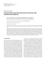
ν
0
λ
0
K
λ
0
e
iα
K
λ
0
−K μ
0
λ
1
−K
−2
2cosα
2
fλ
λ
1
e
iα
K μ
1
, λ
1,2
K λ
2
e
iα
K
λ
2
−K
λ
Figure 1: The graph of fλ.
Suppose that fλ2or−2 for some λ
/
μ
k
0 ≤ k ≤ N
s
, we have k
12
Δψ
N−1
λ −
k
22
ψ
N−1
λ
/
0. From the above discussions again, λ is a simple eigenvalue of 1.1 and 1.2
with α 0orα π,andδ
j
is not identically zero for 0 ≤ j ≤ N − 1.
For this λ
/
μ
k
0 ≤ k ≤ N
s
, 3.39 implies that fλ
/
0, and from Proposition 3.5
i, ii that fμ
0
≤−2, fν
0
≥ 2. Hence, fλ < 0, where ν
0
<λ<μ
0
. It follows from
Proposition 3.5 i that fμ
k
fμ
k1
≤−4and−1
k
fλ > 0, where μ
k
<λ<μ
k1
0 ≤ k ≤
N −3.ByProposition 3.5 i, iii, fμ
N−2
≥ 2 and there exists μ
N−2
<ξ
0
such that fξ
0
≤−2
if N is odd, and fμ
N−2
≤−2 and there exists μ
N−2
<η
0
such that fη
0
≥ 2ifN is even.
Hence, −1
N−2
fλ > 0 where μ
N−2
<λ. This completes the proof.
Proposition 3.7. For any fixed α
/
0, −π<α<π, each eigenvalue of 1.1 and 1.2 is simple.
Proof. Fix α, −π<α<πwith α
/
0. Suppose that λ is an eigenvalue of the problem 1.1 and
1.2.ByProposition 3.3, we have f
2
λ4 cos
2
α<4. It follows from 3.33 that det Iλ > 0
and the matrix Iλ is positive definite or negative definite. Hence, δ
j
> 0for0≤ j ≤ N −1or
δ
j
< 0for0≤ j ≤ N − 1sinceϕ
n
and ψ
n
are linearly independent.
If λ is a multiple eigenvalue of problem 1.1 and 1.2, then 3.5 holds by
Proposition 3.3.Byusing3.5, it can be easily verified that 3.34 holds, that is, all the entries
of the matrix Iλ are zero. Then δ
j
0for0≤ j ≤ N − 1, which is contrary to δ
j
/
0for
0 ≤ j ≤ N −1. Hence, λ is a simple eigenvalue of 1.1 and 1.2. This completes the proof.
Proposition 3.8. Assume that k
11
> 0,k
12
≤ 0 or k
11
≥ 0,k
12
< 0.Ifk is odd, fμ
k
2,
and f
μ
k
0, then f
μ
k
< 0;ifk is even, fμ
k
−2, and f
μ
k
0, then f
μ
k
> 0 for
0 ≤ k ≤ N − 2.
Proof. We first prove the first result. Suppose that k is odd, fμ
k
2, and fμ
k
0.
Then μ
k
is a multiple eigenvalue of 1.1 and 1.2 with α 0byProposition 3.6. Then by
Proposition 3.3, 3.5 holds for λ μ
k
and α 0, that is,
ϕ
N−1
μ
k
k
11
− k
12
, Δϕ
N−1
μ
k
k
21
− k
22
,
ψ
N−1
μ
k
k
12
, Δψ
N−1
μ
k
k
22
.
3.40
Advances in Difference Equations 15
Differentiating fλ with respect to λ two times, we get
f
μ
k
k
22
ϕ
N−1
μ
k
k
11
− k
12
Δψ
N−1
μ
k
−
k
21
− k
22
ψ
N−1
μ
k
− k
12
Δϕ
N−1
μ
k
.
3.41
Differentiating 2.14 with respect to λ two times and from 3.40,weget
−
k
22
ϕ
N−1
μ
k
k
11
− k
12
Δψ
N−1
μ
k
−
k
21
− k
22
ψ
N−1
μ
k
− k
12
Δϕ
N−1
μ
k
2
ϕ
N
μ
k
ψ
N−1
μ
k
− ϕ
N−1
μ
k
ψ
N
μ
k
0,
3.42
which, together with 3.41, implies that
f
μ
k
2
ϕ
N
μ
k
ψ
N−1
μ
k
− ϕ
N−1
μ
k
ψ
N
μ
k
. 3.43
On the other hand, it follows from 3.29 and 2.14 that, not indicating μ
k
explicitly,
ϕ
N
ψ
N−1
− ϕ
N−1
ψ
N
N−1
j0
w
j
ϕ
j
ϕ
N
ψ
j
− ϕ
j
ψ
N
N−2
j0
w
j
ψ
j
ϕ
N−1
ψ
j
− ϕ
j
ψ
N−1
−
N−2
j0
w
j
ϕ
j
ϕ
N−1
ψ
j
− ϕ
j
ψ
N−1
N−1
j0
w
j
ψ
j
ϕ
N
ψ
j
− ϕ
j
ψ
N
⎛
⎝
N−1
j0
w
j
ϕ
j
ψ
j
⎞
⎠
2
−
N−1
j0
w
j
ϕ
2
j
N−1
j0
w
j
ψ
2
j
.
3.44
Since ϕ
n
and ψ
n
are linearly independent on −1,N, the above relation implies that fμ
k
<
0byH
¨
older’s inequality, which proves the first conclusion.
The second conclusion can be shown similarly. Hence, the proof is complete.
Finally, we turn to the proof of Theorem 3.1.
Proof of Theorem 3.1. By Propositions 3.3–3.8, and the intermediate value theorem, one can
obtain the graph of f see Figure 1, which implies the results of Theorem 3.1. We now give
its detailed proof.
By Propositions 3.3–3.6, fμ
0
≤−2, fλ < 0 for all λ<μ
0
with −2 ≤ fλ ≤ 2,
and there exists ν
0
<μ
0
such that fν
0
≥ 2. Therefore, by the continuity of fλ and the
intermediate value theorem, 1.1 and 1.2 with α 0 has only one eigenvalue λ
0
K <μ
0
,
1.1 and 1.2 with α π has only one eigenvalue λ
0
−K ≤ μ
0
,and1.1 and 1.2 with
α
/
0, −π<α<πhas only one eigenvalue λ
0
K <λ
0
e
iα
K <λ
0
−K, and they satisfy
ν
0
≤ λ
0
K
<λ
0
e
iα
K
<λ
0
−K
≤ μ
0
. 3.45
Similarly, by Propositions 3.3–3.6, the continuity of fλ, and the intermediate value theorem,
fλ reaches −2, 2 cosα α
/
0, −π<α<π, and 2 exactly one time, respectively, between
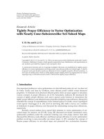
16 Advances in Difference Equations
λ
N−2
−K
λ
N−2
e
iα
K
2cosα
−2
2
fλ
λ
N−2
K μ
N−2
λ
N−1
K λ
N−1
e
iα
K
λ
N−1
−K ξ
0
λ
Figure 2: The graph of fλ in the case that N is odd.
λ
N−2
K λ
N−2
e
iα
K
2cosα
−2
2
fλ
λ
N−2
−K μ
N−2
λ
N−1
−K
λ
N−1
e
iα
K λ
N−1
K η
0
λ
Figure 3: The graph of fλ inthecasethatN is even.
any two consecutive eigenvalues of the separated boundary value problem 1.1 with 2.7.
Hence, 1.1 and 1.2 with α 0; α
/
0, −π<α<π; α πhas only one eigenvalue
between any two consecutive eigenvalues of 1.1 with 2.7, respectively. In addition, by
Proposition 3.6,iffμ
k
2or−2andfμ
k
0, then μ
k
is not only an eigenvalue of 1.1
with 2.7 but also a multiple eigenvalue of 1.1 and 1.2 with α 0andα π.
By Proposition 3.5 i,ifN is odd, fμ
N−2
≥ 2andifN is even, fμ
N−2
≤−2. It
follows 3.22 that if N is odd, then fλ →−∞as λ → ∞, and if N is even, then fλ →
∞as λ → ∞. Hence, if N is odd, then there exists a constant ξ
0
>μ
N−2
such that fξ
0
≤−2,
which, together with Proposition 3.6, implies that 1.1 and 1.2 with α 0; α
/
0, −π<α<π;
α π, has only one eigenvalue λ
N−1
K, λ
N−1
e
iα
K,andλ
N−1
−K, satisfying
μ
N−2
≤ λ
N−1
K
<λ
N−1
e
iα
K
<λ
N−1
−K
≤ ξ
0
3.46
see Figure 2. Similarly, in the other case that N is even, there exists a constant η
0
>μ
N−2
such that fη
0
≥ 2, which, together with Proposition 3.6, implies that 1.1 and 1.2 with
Advances in Difference Equations 17
α 0; α
/
0, −π<α<π; α π has only one eigenvalue λ
N−1
K, λ
N−1
e
iα
K,andλ
N−1
−K,
satisfying
μ
N−2
≤ λ
N−1
−K
<λ
N−1
e
iα
K
<λ
N−1
K
≤ η
0
3.47
see Figure 3. Therefore, we get that 1.1 and 1.2 with α
/
0, −π<α<π,has N eigenvalues
and it is real and satisfies
ν
0
≤ λ
0
K
<λ
0
e
iα
K
<λ
0
−K
≤ μ
0
≤ λ
1
−K
<λ
1
e
iα
K
<λ
1
K
≤ μ
1
≤ λ
2
K
<λ
2
e
iα
K
<λ
2
−K
≤ μ
2
≤ λ
3
−K
<λ
3
e
iα
K
<λ
3
K
≤ μ
3
≤···≤μ
N−3
≤ λ
N−2
−K
<λ
N−2
e
iα
K
<λ
N−2
K
≤ μ
N−2
≤ λ
N−1
K
<λ
N−1
e
iα
K
<λ
N−1
−K
≤ ξ
0
, if N is odd,
ν
0
≤ λ
0
K
<λ
0
e
iα
K
<λ
0
−K
≤ μ
0
≤ λ
1
−K
<λ
1
e
iα
K
<λ
1
K
≤ μ
1
≤ λ
2
K
<λ
2
e
iα
K
<λ
2
−K
≤ μ
2
≤ λ
3
−K
<λ
3
e
iα
K
<λ
3
K
≤ μ
3
≤···≤μ
N−3
≤ λ
N−2
K
<λ
N−2
e
iα
K
<λ
N−2
−K
≤ μ
N−2
≤ λ
N−1
−K
<λ
N−1
e
iα
K
<λ
N−1
K
≤ η
0
, if N is even.
3.48
This completes the proof.
Remark 3.9. Let K I,thatis,k
11
k
22
1, k
12
k
21
0. Then fλϕ
N−1
λψ
N
λ.
In this case, Propositions 3.5 and 3.8 are the same as those mentioned in 4, Propositions 3.1,
3.3–3.5, respectively, and most of the results of Proposition 3.6 are the same as the results of
4,Proposition3.2.
Acknowledgments
Many thanks to Johnny Henderson the editor and the anonymous reviewers for helpful
comments and suggestions. This research was supported by the Natural Scientific Foundation
of Shandong Province Grant Y2007A27, Grant Y2008A28, and the Fund of Doctoral
Program Research of University of Jinan B0621.
References
1 F. V. Atkinson, Discrete and Continuous Boundary Problems, vol. 8 of Mathematics in Science and
Engineering, Academic Press, New York, NY, USA, 1964.
2 Y. Shi and S. Chen, “Spectral theory of second-order vector difference equations,” Journal of
Mathematical Analysis and Applications, vol. 239, no. 2, pp. 195–212, 1999.
3 R . P. A g a r w a l a n d P. J . Y. Wo n g , Advanced Topics in Difference Equations, vol. 404 of Mathematics and Its
Applications, Kluwer Academic Publishers, Dordrecht, The Netherlands, 1997.
18 Advances in Difference Equations
4 Y. Wang and Y. Shi, “Eigenvalues of second-order difference equations with periodic and antiperiodic
boundary conditions,” Journal of Mathematical Analysis and Applications, vol. 309, no. 1, pp. 56–69, 2005.
5 E. A. Coddington and N. Levinson, Theory of Ordinary Differential Equations, McGraw-Hill, New York,
NY, USA, 1955.
6 J. K. Hale, Ordinary Differential Equations, vol. 20 of Pure and Applied Mathematics, Wiley-Interscience,
New York, NY, USA, 1969.
7 W. Magnus and S. Winkler, Hill’s Equation, Interscience Tracts in Pure and Applied Mathematics, no.
20, Wiley-Interscience, New York, NY, USA, 1966.
8 M. Zhang, “The rotation number approach to eigenvalues of the one-dimensional p-Laplacian with
periodic potentials,” Journal of the London Mathematical Society, vol. 64, no. 1, pp. 125–143, 2001.
9 R. P. Agarwal, M. Bohner, and P. J. Y. Wong, “Sturm-Liouville eigenvalue problems on time scales,”
Applied Mathematics and Computation, vol. 99, no. 2-3, pp. 153–166, 1999.