Báo cáo hóa học: " Research Article Tracking Intermittently Speaking Multiple Speakers Using a Particle Filter" doc

Hindawi Publishing Corporation
EURASIP Journal on Audio, Speech, and Music Processing
Volume 2009, Article ID 673202, 11 pages
doi:10.1155/2009/673202
Research Article
Tracking Intermittently Speaking Multiple Sp eakers Using
a Particle Filter
Angela Quinlan, Mitsuru Kawamoto (EURASIP Member), Yosuke Matsusaka, Hideki Asoh,
and Futoshi Asano
Central 2, 1-1-1 Umezono, Tsukuba, Ibaraki 305-8568, Japan
Correspondence should be addressed to Mitsuru Kawamoto,
Received 10 August 2008; Revised 5 March 2009; Accepted 15 May 2009
Recommended by Christophe D’Alessandro
The problem of tracking multiple intermittently speaking speakers is difficult as some distinct problems must be addressed. The
number of active speakers must be estimated, these active speakers must be identified, and the locations of all speakers including
inactive speakers must be tracked. In this paper we propose a method for tracking intermittently speaking multiple speakers using
a particle filter. In the proposed algorithm the number of active speakers is firstly estimated based on the Exponential Fitting Test
(EFT), a source number estimation technique which we have proposed. The locations of the speakers are then tracked using a
particle filtering framework within which the decomposed likelihood is used in order to decouple the observed audio signal and
associate each element of the decomposed signal with an active speaker. The tracking accuracy is then further improved by the
inclusion of a silence region detection step and estimation of the noise-only covariance matrix. The method was evaluated using
live recordings of 3 speakers and the results show that the method produces highly accurate tracking results.
Copyright © 2009 Angela Quinlan et al. This is an open access article distributed under the Creative Commons Attribution
License, which permits unrestricted use, distribution, and reproduction in any medium, provided the original work is properly
cited.
1. Introduction
The ability to track the locations of intermittently speaking
multiple speakers in the presence of background noise and
reverberation is of great interest due to the vast number of
potential applications. In the traditional approach to this
problem, firstly the location of each speaker is estimated

using a sound source localization method such as the MUSIC
or time-delay of arrival (TDOA) methods, and then the
estimated locations (contacts) are used as inputs to the
tracking process using a Kalman filter or extended Kalman
filter. In addition, in order to track multiple targets, a
data association technique such as Joint Probability Data
Association (JPDA) is exploited to bind each estimated
location to a target [1].
Recently, the framework of Bayesian unified tracking has
been applied to the multiple-target tracking problem [2].
In this framework, the location of a target is not explicitly
estimated. Instead, the location estimation, data association,
and tracking are simultaneously solved by combining an
observation model with a motion model. Moreover, in this
framework, a Kalman or extended Kalman filter is not used
because the tracking process treats raw input signals from
array sensors directly, instead of using the estimated contacts
as inputs.
Under these circumstances particle filtering techniques
are often applied, and in recent years, some authors have
reported the application of these techniques to tracking
audio sources, for example, [3, 4]. Using the particle filtering
approach, the probability distribution of the estimated
locations of the sources being tracked is approximated with
a distribution of a state vector of particles and the state
of each particle is recursively updated. The prediction step
uses prior information about each source’s previous location
together with a predefined motion model (usually a random
walk, which is a simple model and one that allows us to
evaluate the performance of the particle algorithm itself), to

predict the current locations of the sources. This “prediction-
likelihood” is then weighted using received microphone
signals, through the measurement likelihood, and particles
2 EURASIP Journal on Audio, Speech, and Music Processing
are resampled according to their weights to obtain the
posterior distribution from which the location estimate can
be found.
The incorporation of any prior knowledge into this
framework allows for more robust tracking as seen in [3],
where the application of Time Delay Estimation (TDE)
within a particle filtering framework provides improved
robustness to spurious peaks in the correlation caused
by reverberation and background noise. As well as this
increased robustness the number of data samples required
by particle filtering methods is less than that required for
high resolution techniques such as MUSIC [5]. This is a
particularly important point when tracking moving sources.
While various particle filtering methods have been
applied to the problem of tracking a single speaker, the
extension of these techniques to the case of multiple speakers
is not straightforward. This is mainly due to the fact that
one or more of the speakers may not be speaking at any
given moment, making it necessary to estimate the number
of “active” speakers and also which particular speakers are
active at that time.
In the literature this problem is solved by introduc-
ing hidden variables which represent the status of each
speaker. Then the particle filter is applied to solve the
joint problem of estimating the speaker status and tracking
the locations of speakers [6, 7]. However, this approach

leads to greater computational complexity as the number of
speakers increases. Therefore in this paper we instead use
an alternative approach of firstly estimating the number of
active speakers and then using the particle filter to perform
the tracking of their locations.
In order to estimate the number of active speakers, we
introduce a method based on the Exponential Fitting Test
(EFT), a source number estimation technique proposed in
[8] and which is extended to allow for the presence of
reverberation in [9]. Identification of the active speakers
is then performed. Finally, all speakers, including inactive
speakers who are silent for some periods of time during the
recording process are tracked using a particle filter.
It should be noted that once a speaker becomes inactive,
he can no longer be tracked. However, using the state
transition probability, an estimate of an inactive speaker
location can be retained, which is an advantage in updating
the speaker location once the speaker becomes active again.
A block diagram for the proposed algorithm is shown
in Figure 1. Live recordings are used, firstly, to evaluate
the tracking algorithm and then, secondly, to evaluate the
performance of the proposed speaker activity detection step.
2. Problem Formulation
In this paper we investigate the problem of tracking the
location of N
s
moving speakers using an array of M
microphones. Each speaker speaks intermittently. The audio
signal is treated in the frequency domain. The short-time
Fourier transform (STFT) of the M microphone inputs is

denoted as
y
(
ω, t
)
=

y
1
(ω, t), , y
M
(ω, t)

T
,(1)
Estimate noise-only covariance matrix
Correct the eigenvalues of
the noise-only covariance
matrix with a correction
factor
Estimate number of
active speakers
Evaluate decomposed likelihood
and identify active speakers
Evaluate measurement likelihood
and particle filter tracking
Tracking
results
Y(k)
Figure 1: Block diagram for the proposed algorithm.

where y
m
(ω, t) denotes the STFT of the mth microphone
input at time t and frequency ω, and the superscript T
denotes the transpose of a vector or a matrix. We estimate
the location of speakers every N STFT frames. A processing
data block is denoted as
Y
(
ω, k
)
=

y
(
ω, t
0
)
, , y
(
ω, t
0
+ N − 1
)

,(2)
where t
0
is the start time of the kth block.
Let Y(k)andΘ(k) denote the entire data in the kth block

and the locations of the N
s
speakers, respectively. That is
Y
(
k
)
={Y
(
ω
min
, k
)
, , Y
(
ω
max
, k
)
},
Θ
(
k
)
=

θ
1
(
k

)
, , θ
N
s
(
k
)

,
(3)
where ω
min
and ω
max
are the lowest and highest frequencies
respectively. Then our problem is to estimate Θ(k) using
observed data Y
1|k
={Y(1), , Y(k)}.
2.1. Bayesian Multiple Target Tracking. We treat the problem
within the framework of Bayesian tracking theory [2]. In this
framework, the tracking problem is reduced to calculating
the posterior probability distribution p(Θ(k)
| Y
1|k
)ofthe
target variable Θ(k) given the observation Y
1|k
. We introduce
the standard Markov assumption about the movement of the

speakers and the observation process. That is, we assume that
the following recursive equation holds for all k:
p

Θ
(
k
)
| Y
1|k

=
1
Z
p

Y
(
k
)
| Θ
(
k
)


p
(
Θ
(

k
)
| Θ
(
k − 1
))
× p

Θ
(
k − 1
)
| Y
1|k−1

d Θ
(
k − 1
)
,
(4)
where Z is the normalization constant, p(Y(k)
| Θ(k)) is the
measurement likelihood (observation model), and p(Θ(k)
|
Θ(k − 1)) is the state transition probability (motion model).
EURASIP Journal on Audio, Speech, and Music Processing 3
2.2. Particle Filters. In general, computing the integral
according to Θ(k
− 1) in (4) is analytically impossible for

nonlinear observation/motion models. The usual numerical
integration becomes intractable as the number of speakers
N
s
increases because the dimension of the integrated vari-
able space increases and the computational cost increases
exponentially. The particle filter is a popular approach
to calculate the posterior distribution approximately for
nonlinear models [10].
The posterior distribution of the target variable Θ(k)is
approximated by the distribution of a number of weighted
discrete points, that is, particles. The ith particle is associated
with a state value of Θ
i
(k)andaweightvaluew
i
called “the
importance” of the particle. Then the empirical probability
density of Θ is defined as
p
emp
(
Θ
(
k
))
=
1
N
p

N
p

i=1
w
i
δ

Θ
(
k
)
− Θ
i
(
k
)

,(5)
where N
p
is the number of particles and δ(x)isDirac’s
delta function. If the particles are correctly distributed, then
according to Kolmogorov’s strong law of large numbers,
as the number of particles increases toward infinity the
empirical distribution approaches the true posterior density.
A recursive step of the simplest particle filtering algo-
rithm for computing the posterior p(Θ(k)
| Y
1|k

)isas
follows.
(1) Let a set of particles and weights for the k
− 1th block
{Θ
i
(k − 1), w
i
(k − 1), i = 1, , N
p
} be given.
(2) Generate a new set of particles
{Θ
i
(k)} by propa-
gating the particles according to the motion model
p(Θ(k)
| Θ(k − 1)).
(3) Compute the measurement likelihood p(Y(k)
|
Θ
i
(k)) for each particle.
(4) Revise the weight values as w
i
(k) = p(Y(k) |
Θ
i
(k))w
i

(k − 1) and normalize the weights as

i
w
i
(k) = 1.
(5) Resample particles in proportion to the weight values
and reset all weights as 1/N
p
.
Hence, for implementing the basic particle filter, only the
evaluation of the measurement likelihood for each particle
is necessary.
The final estimate of the source locations can then be
obtained by maximizing the posterior probability distribu-
tion (MAP estimate), or by taking the weighted mean over
the particles as

Θ(k) =
1
N
p
N
p

i=1
w
i
Θ
i

(
k
)
. (6)
This yields an approximation of the expectation of Θ(k)
under the posterior p(Θ(k)
| Y
1|k
), which is called the
minimum mean-square error (MMSE) estimate. In this
research, we used the MMSE estimate.
2.3. The Problem of Intermittent Speech. So far we have
explained the standard procedure for Bayesian multiple
target tracking. The main difficulty with our problem comes
from the fact that speakers speak intermittently. This means
that the measurement likelihood p(Y(k)
| Θ(k)) changes
depending on the status of each speaker, that is, which
speakers are active in the kth block.
In previous studies this problem has been solved by
introducing hidden variables which represent the status of
each speaker. Then a particle filter is applied to solve the
joint problem of estimating the speaker status and tracking
the locations of speakers [6, 7]. However this approach
turns out to require large numbers of particles when the
number of speakers increases, in order to estimate the
active speakers using a particle filter, because the number
of possible combinations of active and inactive speakers
increases exponentially. This property is not suitable for real-
time applications.

In this paper we instead propose an alternative approach
of firstly estimating the number of active speakers and
identifying them, then using a particle filter to perform the
tracking. With this approach, the particle filter is not used
to track the combinatorial speakers’ status and the number
of particles can be reduced. In addition, we introduce online
estimation of the noise covariance matrix based on detection
of the silence region (for details of the detection method,
see Section 3.2). Figure 1 depicts a block diagram of the
overall tracking process. Each step is explained in detail in
the following sections.
3. Noise-Only Covariance Estimation
As the first step, the noise-only frequency subbands are
identified by a pause detection technique, and the noise-only
covariance matrix is estimated. In order to determine the
number of speakers, we need the eigenvalues of the noise-
plus-reverberation matrix. However, this matrix is unknown.
Instead, since we can estimate the noise-only covariance
matrix, we consider obtaining a better approximation to
the true noise-plus-reverberation eigenvalues by correcting
the eigenvalues of the noise-only covariance matrix with
a correction factor. The correction factor is discussed in
Section 4. Therefore, in this section, we propose a method
for estimating the noise-only covariance matrix.
3.1. Signal Model. We denote the number of active speakers
by N
a
. The microphone input y(ω, t)forN
a
directional

signals s(ω, t)plusbackgroundnoisen(ω, t) is modeled as
y
(
ω, t
)
= A
(
ω, k
)
s
(
ω, t
)
+ n
(
ω, t
)
,(7)
where A(ω, k) is the matrix composed of the N
a
direct path
transfer function vectors:
A
(
ω, k
)
=

a
1

(
ω, k
)
, , a
N
a
(
ω, k
)

. (8)
Here we assume that A is constant during a processing data
block, that is, A depends only on k. This assumption is
satisfied when N, the size of the processing block, is small
4 EURASIP Journal on Audio, Speech, and Music Processing
enough. In the experiment below, we set N equal to 9;
this means that the block length is 0.1 second, where the
time 0.1 second is derived from the experimental conditions
shown in Tabl e 1 in Section 6. Each transfer function vector
is
a
l
(
ω, k
)
=

e
− jωτ
1l

(k)
a
1l
(
k
)
, , e
− jωτ
Ml
(k)
a
Ml
(
k
)

,(9)
where a
ml
(k)andτ
ml
(k) denote the gain and the time
delay, respectively, between the lth speaker and the mth
microphone. s(ω, t)
= [s
1
(ω, t), , s
N
a
(ω, t)]

T
is the source
spectrum vector, and n(ω, t)
= [n
1
(ω, t), , n
M
(ω, t)]
T
is
the background noise spectrum vector.
Normally it is assumed that the signal and noise are
uncorrelated and that the noise is Gaussian with known
power. However, in most practical situations this assumption
will not hold because of the existence of reverberation, and it
is shown in [11] that it leads to degraded tracking results.
It is therefore desirable to use a more accurate model of the
background noise.
3.2. Determination of Silence Regions of Speakers. We fir st
detect the noise-only subbands based on the noise charac-
terization method proposed in [12], in which a threshold is
applied to each frequency subband in order to distinguish
between frequencies containing only noise and frequencies
containing speech components.The energy of a subband ω
for the kth block is defined as
E
(
ω, k
)
=

1
N
t
0
+N−1

t=t
0
y
(
ω, t
)
H
y
(
ω, t
)
, (10)
where the superscript H denotes the conjugate transpose of
the matrix. The noise threshold η(ω, k) is calculated as
η
(
ω, k
)
= βE
n
(
ω, k
− 1
)

, (11)
where β is a constant value lying between 1.5and2.5which
can be chosen during the training period. E
n
(ω, k − 1) is the
energy of the previous noise estimate at the given frequency
ω and it is determined by averaging the previous noise energy
values at this frequency over a specified time period.
A decision is then made as to whether or not each
frequency subband contains the required target signal. If the
power of the subband E(ω, k)satisfiesE(ω, k)
≤ η(ω, k), the
frequency value ω is determined as a noise-only subband and
E
n
(ω, k) is updated using E(ω, k). Otherwise, ω is considered
to contain signal components, and E
n
(ω, k) is not updated
(E
n
(ω, k) = E
n
(ω, k − 1)). This allows the noise power
estimate to be continuously updated on a frequency-by-
frequency basis, even while someone is speaking.
3.3. Calculate Noise-Only Covariance Matrix. The noise-only
covariance matrix estimate for a frequency subband ω can be
defined as
C

n
(
ω, k
)
=
1
N
t
0
+N−1

t=t
0
n
(
ω, t
)
n
H
(
ω, t
)
. (12)
If E(ω, k) <η(ω, k), the frequency subband is determined
to contain no signal component. This means that y(ω, t)
=
n(ω, t) and the estimate of the covariance can be computed
as
C
n

=
1
N
t
0
+N−1

t=t
0
y
(
ω, t
)
y
H
(
ω, t
)
. (13)
The resulting covariance estimate is then smoothed over
some period of time in order to stabilize the estimate

C
n
(
ω, k
)
=
1
Q

k

q=k−Q+1
C
n

ω, q

, (14)
where Q is the number of previous values used for smooth-
ing.
4. Estimation of the Number of Active Speakers
The second step is estimating the number of active speakers
N
a
. For sound source number estimation, statistical model
selection criteria such as the Minimum Description Length
(MDL) [13] and Akaike’s Information Criterion (AIC) [14]
are traditionally used. However, both these approaches are
based on an assumption of white noise and are known
to consistently overestimate the number of sources present
when reverberation is present [15].
In what follows we use the method proposed in [8],
extended to cover reverberant environments as detailed in
[9]. The method is based on analyzing the eigenvalues of the
covariance matrix of input signals. Hereinafter, we describe
the procedure for a frequency subband ω in a processing
block k. The index of the block k and the index of the
subband frequency ω are omitted for the sake of simplicity
where they are unnecessary.

The spatial correlation matrix K
y
of the received signals
is defined as
K
y
= E

y
(
t
)
y
H
(
t
)

, (15)
where E[
···] denotes taking the average over time. Using
the signal model (7), the covariance can be written as
K
y
= AK
s
A
H
+ K
n

, (16)
where
K
s
= E

s
(
t
)
s
H
(
t
)

,
K
n
= E

n
(
t
)
n
H
(
t
)


.
(17)
As is described in the previous section, normally it is
assumed that the signal and the noise are uncorrelated. Then
the covariance matrices become
K
s
= diag

γ
1
, , γ
N
a

. (18)
Here, diag
{···} denotes a diagonal matrix with diagonal
elements
{···} and γ
l
denotes the power of s
l
(t), that
EURASIP Journal on Audio, Speech, and Music Processing 5
is, γ
l
= E[s
l

(t)s
∗
l
(t)], where the superscript
∗
represents
the conjugate. In the same manner, the observed noise is
assumed to be uncorrelated:
K
n
= diag

σ
2
1
, , σ
2
M

, (19)
where σ
2
i
(i = 1, , M) denotes the power of n
i
(t).
If we can assume that all σ
2
i
are equal to σ

2
, the noise
covariance can be written as K
n
= σ
2
I using the M × M
identity matrix I.Then(16) can be reexpressed as:
K
y
= AK
s
A
H
+ σ
2
I, (20)
and the eigenvalues of K
y
are therefore given by
λ
1
, , λ
M
= γ
1
+ σ
2
, , γ
N

a
+ σ
2
, σ
2
, , σ
2
. (21)
The number of eigenvalues corresponding to the signal
subspace, the so-called signal eigenvalues, is equal to the
number of active sources, and assuming that the source
power is greater than that of the background noise, the
number of sources present can now be easily determined as
the number of eigenvalues not equal to σ
2
.
In practice, however, K
y
is unknown and must instead be
estimated using
C
y
=
1
N
t
0
+N−1

t=t

0
y
(
t
)
y
H
(
t
)
. (22)
In this case the active source number estimation problem
still consists of distinguishing between the signal and noise
eigenvalues. However, with the statistical fluctuations in
C
y
, the noise eigenvalues are no longer all equal to σ
2
.In
particular, for moving sources, we cannot take large N and
the fluctuations become larger. The separation between noise
and signal eigenvalues is only clear now in the case of high
Signal-to-Noise Ratio (SNR) and low reverberation, when a
gap can be clearly observed.
In order to distinguish between signal and noise eigen-
values for moving sources conditions, we approximate the
decreasing profile of the eigenvalues of the noise spatial
correlation matrix

C

n
, and compare this to the profile of the
observed eigenvalues of C
y
. It is known that a decreasing
profile can be approximated using the first- and second-order
moments of the eigenvalues together with an initial assump-
tion of white noise [8]. The smallest observed eigenvalue λ
M
is assumed to be a noise eigenvalue, corresponding to a noise
subspace dimension of d
= 1. Then incrementing d by 1 for
each subsequent step until d
= M − 1, the predicted profile
of the noise only eigenvalues is found recursively using

λ
M−d
=
(
d +1
)
J
d+1
σ
2
(23)
where
J
P+1

=
1 − r
d+1,N
1 −

r
d+1,N

d+1
,
σ
2
=
1
d +1
d

i=0
λ
M−i
,
r
m,n
= e
−2ξ
m,n
,
(24)
ξ
m,n

=




1
2

15
m
2
+2
−

225
(
m
2
+2
)
2
−
180m
n
(
m
2
− 1
)(
m

2
+2
)

.
(25)
The relative differences between the predicted and
observed mth eigenvalue profiles δ
m
are calculated using
δ
m
=
λ
m
−

λ
m

λ
m
, m = 1, , M − 1, (26)
and δ
m
is then compared to a threshold value η
m
in order to
distinguish the signal eigenvalues. These threshold values η
m

for m = 1, 2, , M − 1 are selected from the distribution of
the relative differences for each frequency component when
there is only noise present at that frequency (for a discussion
on how to select this threshold value see [9]). Also, for the
details on the derivation of (23) through (25), see [8].
The predicted noise eigenvalue profile

λ
1
, ,

λ
M
is based
on the assumption that the background noise can be
modeled as white noise. This approximation is valid in many
practical situations when none of the speakers are active.
Once some of the speakers are active though, reverberant tails
arising due to the presence of speech violate this white noise
assumption and lead to an increase in the noise eigenvalue
profile.
In this case the noise eigenvalue profile predicted from
(23)–(25) will be lower than that of the observed noise
eigenvalues, resulting in frequent overestimation of the
number of active sources. Therefore once it is known that
at least one speaker is present, it is necessary to apply a
correction factor to the predicted profile in order to account
for the increase in the noise eigenvalues due to reverberation.
In order to calculate a suitable correction factor the
eigenvalues of the estimated reverberation-only correlation

matrix, λ
rev
1
, , λ
rev
M
, are evaluated. These values are then
used to find the corresponding predicted noise eigenvalues

λ
rev
1
, ,

λ
rev
M
as described in (23)–(25). It should be noted
that the reverberation-only correlation matrix is estimated
using impulse responses recorded in the room in which the
tracking is carried out.
The difference between the predicted and observed
profiles, relative to the largest observed eigenvalue, is then
taken as a correction factor:
cf
m
=
λ
rev
m

−

λ
rev
m
λ
rev
1
, m = 2, , M. (27)
In the presence of at least one active source the correction
factor is then used to modify the originally predicted noise
eigenvalue profile:

λ
mod
m
=

λ
m
+ cf
m
λ
1
. (28)
Once again the predicted and observed profiles are compared
by finding their relative difference:
δ
mod
m

=
λ
m
−

λ
mod
m

λ
mod
m
. (29)
6 EURASIP Journal on Audio, Speech, and Music Processing
If δ
mod
m
>η
m
then λ
m
is a signal eigenvalue. The number
of active speakers at this subband is then estimated as the
number of signal eigenvalues. In order to obtain the final
estimate of the number of active speakers for the broad band
signal,

N
a
, the estimate in each subband is averaged over all

active subbands within the frequency range [ω
min
, ω
max
].
5. Evaluating Measurement Likelihood
The third step is identifying the active speakers and eval-
uating the measurement likelihood p(Y
| Θ
i
)foreach
particle. We exploit the random signal model in [16], that
is, we assume that each s(t) is a 0-mean circular complex
Gaussian random vector, with unknown covariance, and
that successive samples of s(t) are independent but share a
common density. We also assume that components of s(t)
are independent of each other; hence the covariance matrix
K
s
is diagonal.
5.1. Decomposing the Likelihood. For a while, we assume
that all N
s
speakers are speaking. Then the log likelihood
function of the observed data Y(ω) given the location of the
N
s
speakers Θ, the signal covariance matrix K
s
(ω), and the

noise covariance matrix K
n
(ω)is
L
y
(
Y
| Θ, K
s
, K
n
)
=−N log



det

K
y




−
1
2
t
0
+N−1


t=t
0
y
H
(
t
)
K
−1
y
y
(
t
)
,
(30)
where we have discarded unnecessary constant terms. As we
described, K
y
can be written as
K
y
= A
(
Θ
)
K
s
A

(
Θ
)
H
+ K
n
, (31)
where
A
(
Θ
)
=

a
(
θ
1
)
, , a

θ
N
s

, (32)
and a(θ
l
) is the transfer function vector for the location
θ

l
. Note that the log likelihood function L
y
is a nonlinear
function of the location parameters Θ. Hence, it is impossible
to apply the Kalman filter to our tracking problem.
Now we introduce a hidden “complete data vector”
x(t)
= [x
T
1
(t), , x
T
N
s
(t)] as in [16] which corresponds to
the signal due to each speaker, and assume that the observed
microphone signals can be decomposed into these signals as
y
(
t
)
=
N
s

l=1
x
l
(

t
)
= Hx
(
t
)
, (33)
where
x
l
(
t
)
= a
(
θ
l
)
s
l
(
t
)
+ n
l
(
t
)
,
H

=
[
I, , I
]
,
(34)
where n
l
(t) is an arbitrary decomposition of the noise vector
n(t), which must satisfy

N
s
l=1
n
l
(t) = n(t).
Then under the assumption of uncorrelated signals, that
is,
K
s
= diag

γ
1
, , γ
N
s

, (35)

the log likelihood of Y can be decomposed into the sum of
the log likelihoods of the individual X
l
= [x
l
(t
0
), , x
l
(t
0
+
N
− 1)] thus
L
y
(
Y
| Θ, K
s
, K
n
)
=
N
s

l=1
L
xl


X
l
| θ
l
, γ
l
, K
nl

. (36)
Here
L
xl

X
l
| θ
l
, γ
l
, K
nl

=−
N log|det
(
K
xl
)

|
−
1
2
t
0
+N−1

t=t
0
x
H
l
(
t
)
K
−1
xl
x
l
(
t
)
,
(37)
K
xl
= γ
l

a
(
θ
l
)
a
H
(
θ
l
)
+ K
nl
,
K
nl
= E

n
l
(
t
)
n
H
l
(
t
)


.
(38)
Using the sample covariance matrix C
xl
of the complete
data X
l
C
xl
=
1
N
t
0
+N−1

t=t
0
x
l
(
t
)
x
H
l
(
t
)
, (39)

the log-likelihood can be rewritten as:
L
xl

X
l
| θ
l
, γ
l
, K
nl

=−N log|det
(
K
xl
)
|
−
N
2
tr

C
xl
K
−1
xl


.
(40)
As the complete data is not known C
xl
cannot be determined
directly. However the correlation matrix can be estimated
using the following equations in the Expectation step of the
EM algorithm in [16]:
C
xl
= E

C
xl
| C
y
;

K
y

=

K
xl
−

K
xl


K
−1
y

K
xl
+

K
xl

K
−1
y
C
y

K
−1
y

K
xl
,
(41)
with

K
y
=

N
s

l=1

K
xl
,

K
xl
= γ
l
a
(
θ
l
)
a
H
(
θ
l
)
+ C
nl
.
(42)
It can be seen that this expression requires
γ

l
,an
estimation of the power of the lth speaker, and C
nl
,an
estimation of the decomposed noise covariance matrix K
nl
.
γ
l
can be estimated from θ
l
using
γ
l
=
a
H
(
θ
l
)
C
y
a
(
θ
l
)
| a

(
θ
l
)
|
4
. (43)
EURASIP Journal on Audio, Speech, and Music Processing 7
Table 1: Experimental parameters.
Sampling frequency 16000 Hz
FFT length 512
FFT shift 128
Frequency range 230–800 Hz
Block length N 9(0.1s)
Q 25 s
N
p
100
β 1.5
Finally the estimate of the decomposed noise covari-
ance matrix C
nl
is given by evenly dividing the noise-
only-reverberant covariance matrix, which is estimated in
Section 3.3, among the number of speakers as:
C
nl
=
1
N

s

C
n
. (44)
This method allows for tracking the sources in situations
where there is no prior knowledge of the background noise,
thus making it much more useful for practical tracking
problems.
Applying the above procedure for all active fre-
quency subbands ω and taking the mean of L
xl
(X
l
(ω) |
θ
l
, γ
l
(ω), C
nl
(ω)), we get the estimated partial log likelihood

L
xl
(X
l
| θ
l
)as


L
xl
(
X
l
| θ
l
)
=
1
| Ω
a
|

ω∈Ω
a
L
xl

X
l
(
ω
)
| θ
l
, γ
l
(

ω
)
, C
nl
(
ω
)

,
(45)
where Ω
a
and | Ω
a
| are the set of active frequency subbands
and the number of active subbands respectively, and X
l
is the
collection of X
l
(ω) for all active subbands.
5.2. Identifying Active Speakers. So far we have assumed that
all N
s
speakersareactive.Whenoneormorespeakersare
inactive, we need to identify the active speakers. In this paper
we identify the active speakers by comparing the values of the
estimated partial likelihood

L

xl
for the lth speaker.
We calculate the average of

L
xl
(X
l
| θ
i
l
) for all particles as
L
xl
=
1
N
p
N
p

i=1

L
xl

X
l
| θ
i

l

, (46)
where θ
i
l
is the lth value of the state vector of the ith particle.
Then the lth speaker which corresponds to the

N
a
largest
values of (46)isdeterminedtobeactive.Here

N
a
is the
estimate of the number of active speakers for the broad band
signal which was given in Section 4. We denote the set of
indices for the active speakers as A.
5.3. Evaluating Likelihood. As the measurement likelihood
of the audio input is irrelevant for the location of inactive
speakers, the total log likelihood for the ith particle can
be obtained by taking the sum of the decomposed log
likelihoods only for active speakers as

L
y

Y | Θ

i

=

l∈A

L
xl

X
l
| θ
i
l

. (47)
Then the measurement likelihood for the ith particle is
obtained as
p

Y | Θ
i

=
exp


L
y


Y | Θ
i

. (48)
Using this likelihood, we can execute the particle filtering
algorithm described in Section 2.2, and compute the estimate
of the source location for the target processing block using
the (6).
6. Experimental Results
The proposed tracking method was tested using recordings
taken in a medium sized meeting room (585 m
× 885 m)
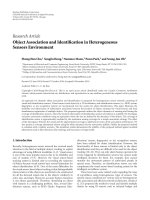
with a reverberation time of 500 millisecond. As shown
in Figure 2, three people, one female and two males,
moved around the room, while speaking intermittently. The
speech was recorded using a uniform circular array of 8
microphones which was placed at ceiling height, and the
distance between the microphone array and the speakers was
sufficient to ensure far-field conditions. The recorded signals
were divided into frames of length 32 millisecond, with an
averaging interval of N
= 9(blocklength),orapproximately
0.1 second. The experimental parameters are given in Tabl e 1.
We note that the rates of the time intervals for the cases
when only one speaker, two speakers, and three speakers are
speaking are 15.6%, 48.3%, and 31.7%, respectively. The time
intervals for the case when no speaker is active is only 4.4%.
This means that the time during which multiple speakers are
speaking simultaneously is rather long in the data. Moreover,
the average times of a silence (inactive) region for speakers

P1, P2, and P3 are 0.48 second, 0.26 second, and 0.93 second,
respectively.
The true trajectory of the speakers was found using a
zone positioning system ZPS-3D by Furukawa Co., Ltd. and
is depicted by the dashed lines in Figure 2(a) and Figures 3,
4,and5, which shows the experimental layout. Using the
zone positioning system, a badge is pinned on the chest of
each of the speakers and the location of the badge is then
tracked. According to the specification of the system, the
measurement accuracy is 20 to 80 mm depending on the
environment and the measured distance.
In the following subsections we will describe the results of
three experiments using the data. In Section 6.1 the accuracy
of the proposed tracking method is evaluated using the Root
Mean Square Error (RMSE) between the true trajectory and
the estimated trajectory. Three kinds of noise covariance
matrix, simply assuming white noise, using an estimate
of the noise covariance matrix, and using modified noise
covariance, are tested and compared. In Section 6.2, tracking
results using two pseudolikelihood functions instead of (40)
are shown for comparison purposes. In Section 6.3, the
accuracy of the speech event detection by the proposed active
8 EURASIP Journal on Audio, Speech, and Music Processing
Table 2: Root Mean Square Error (RMSE) values for the case where the active speakers are estimated, where the RMSE values are calculated
from distance estimation in meters (m). The headings “Total” and “Active” denote the error for the entire tracking time and for the time that
each speaker was determined to be active, respectively.
White noise RMSE Estimated noise RMSE
Error
Total (m) Active (m) Total (m) Active (m)
Speaker 1

0.78 0.51 1.11 0.78
Speaker 2
0.80 0.61 1.02 0.74
Speaker 3
2.0 1.16 1.06 0.61
Average over 3 speakers
1.19 0.76 1.06 0.71
PC, desk
and chair
Chair and
table
Large TV
screen
Microphone array
Door
P2
P1
P3
(a) The three people are denoted P1, P2, P3, and the
dashed line traces their movements. The microphone
array is set at ceiling height
(b) Video image taken during recordings
Figure 2: Experimental layout.
0123456
x-coordinate (m)
1
2
3
4
5

6
y-coordinate (m)
Speaker 1
Speaker 2
Speaker 3
(a) Measurement likelihood found using the proposed algorithm,
Background noise assumed white.
0123456
x-coordinate (m)
1
2
3
4
5
6
y-coordinate (m)
Speaker 1
Speaker 2
Speaker 3
(b) Measurement likelihood found using the proposed algorithm,
Estimated background noise.
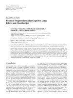
Figure 3: Tracking results. The dashed lines represent the trace of the actual motions.
EURASIP Journal on Audio, Speech, and Music Processing 9
Table 3: RMSE values for the case where all the diagonal elements
of C
nl
are the same constant value, where the RMSE values are
calculated from distance estimation in meters (m).
RMSE
Error Total (m) Active (m)

Speaker 1 0.76 0.50
Speaker 2 0.90 0.68
Speaker 3 1.21 0.67
Average over 3 speakers 0.96 0.62
0123456
x-coordinate (m)
1
2
3
4
5
6
y-coordinate (m)
Speaker 1
Speaker 2
Speaker 3
Figure 4: The tracking result (estimated covariance matrix of
background noise, but the diagonal elements of the matrix are a
constant value). The dashed lines represent the trace of the actual
motions.
speaker identification step is evaluated because one of the
main applications of the proposed method is envisaged as
preprocessing for speech recognition.
6.1. Tracking Experiments. We will show the results when the
number of active speakers is estimated at each time step and
the silence region detection step is included to eliminate the
noise only frequencies. The results for this case are shown
in Figure 3, and the corresponding Root Mean Square Error
(RMSE) values are shown in Ta ble 2.
Figure 3(a) shows the case where the measurement

likelihood is calculated using (48) and the background noise
is assumed white. Figure 3(b) shows the result when the
measurement likelihood is calculated using (48) and the
noise covariance is estimated from the received data using
(14)and(44).
An inactive speaker location can no longer be tracked,
but using the state transition probability, an estimate of an
inactive speaker location can be kept, which is an advantage
in updating the speaker location, once the speaker becomes
active again. Therefore, the location estimates of the inactive
speakers cannot be expected to be very accurate. For this
reason we demonstrate the RMSE values for both the entire
data (total) and the time intervals that each speaker was
determined to be active(active) in Table 2.
From Tabl e 2, the average performance for the estimated
noise case is better than that for the white noise case. This is
because the performance of tracking Speaker 3 is improved
by estimating the noise covariance matrix, C
nl
.However,the
performances of tracking Speakers 1 and 2 for the estimated
noise case became worse than those for the white noise case.
As a method of improving the result, we tried changing
all the diagonal elements of C
nl
to the same constant value
(say, 0.1). The tracking result is shown in Figure 4 and the
RMSE values are shown in Tabl e 3. From the figure and table,
one can see that the performances of tracking Speakers 1
and 2 are close to those for the white noise case and the

performance of tracking Speaker 3 is close to that for the case
of estimated noise.
From all the results, we conclude that the tracking
performance is improved by estimating C
nl
, but that if
the performance is not improved, it would be advisable to
change all the diagonal elements of C
nl
to the same constant
value. It should be noted that the nondiagonal elements of
C
nl
are unchanged.
6.2. Other Likelihood Functions. For comparison purposes
we then considered the same situation but this time the
power spectrum as calculated using MUSIC and the energy
from TDOA [17], as calculated using R
τ
in (49), were instead
used as a pseudolikelihood function for the current tracking
method:
R
τ
=
M

i=1
M


j=i+1
R
ij


τ
ij

,
R
ij
(
τ
)
=
1
N
fl
N
fl
−1

k=0
y
i
(
ω
k
)
y

∗
j
(
ω
k
)
| y
i
(
ω
k
)
y
∗
j
(
ω
k
)
|
e
jω
k
τ
,
(49)
where
τ
ij
= max

τ
R
ij
(τ)andω
k
= 2πk/N
fl
.
Figures 5(a) and 5(b) show the results obtained by using
MUSIC and TDOA, respectively. Tab le 4 shows the RMSE
values of the results. From the results in Figures 5(a) and
5(b), MUSIC and TDOA can track at most, respectively,
two speakers and one speaker. This might be because the
power spectrum of MUSIC and the energy of TDOA are
calculated detecting all speakers. Namely, the observations
y(ω, t), which include the information on all speakers, are
used to calculate the likelihood function. On the other hand,
the likelihood function of the proposed method is calculated
for each speaker, using x
l
(t)in(34) which includes the
information on each active speaker. Therefore we conclude
that the proposed method using (48) is more suitable for
tracking multiple speakers. Note that we are able to confirm
that, even if the number of speakers is four, the proposed
method can track each speaker [18].
10 EURASIP Journal on Audio, Speech, and Music Processing
Table 4: RMSE values for the results obtained by MUSIC and TDOA, where the RMSE values are calculated from distance estimation in
meters (m).
MUSIC RMSE TDOA RMSE

Error Total (m) Active (m) Total (m) Active (m)
Speaker 1 1.31 0.92 2.46 1.81
Speaker 2 1.11 0.81 1.87 1.41
Speaker 3 2.59 1.56 2.88 1.79
Average Over 3 Speakers 1.67 1.10 2.40 1.67
0123456
x-coordinate (m)
1
2
3
4
5
6
y-coordinate (m)
Speaker 1
Speaker 2
Speaker 3
(a) Measurement likelihood found using MUSIC
0123456
x-coordinate (m)
1
2
3
4
5
6
y-coordinate (m)
Speaker 1
Speaker 2
Speaker 3

(b) Measurement likelihood found using TDOA
Figure 5: Tracking results. The dashed lines represent the trace of the actual motions.
Table 5: Speaker activity detection results.
Speaker Speaker Speaker Average
1% 2% 3% %
Speaker state correctly
detected
73.11 58.09 50.29 60.50
Speaker incorrectly
determined active
19.83 15.19 20.10 14.38
Speaker incorrectly
determined inactive
7.05 26.72 29.63 21.13
6.3. Speech Event Detection. In this subsection, the perfor-
mance of the active speaker identification step is investigated.
While the recording in the experiment was being carried out,
a lapel microphone was attached to each speaker so that the
true period of each speech event could be hand labeled by
human listeners. This labeling was then compared to the
results found by the proposed active speaker identification
method.
From the results given in Ta bl e 5 it can be seen that
the mean rate of correct determination of the activity state
is approximately 60%, with Speaker 3 having the lowest
correct determination rate of 50.29%. However, since the
incorrect determined active rate is low, we consider that
the proposed active speaker identification method works
well. Regarding the incorrectly determined inactive speakers,
from the analysis of the speech segments, it turned out

that there exists a situation where the speech volume is
low or noisy, although the speaker is active. The incorrectly
determined inactive rate is somewhat high for Speakers 2 and
3. These resultsreflect the fact that the speech volume levels
ofSpeakers2and3arelowerthanSpeaker1.
7. Conclusion
This paper proposes a novel scheme for tracking intermit-
tently speaking multiple speakers. In the proposed tracking
method, the number of active speakers can be estimated
using the observed covariance matrix and the estimated
noise-only-reverberant covariance matrix (see Section 3).
Then the active speakers are identified using the decomposed
likelihood function. Finally all speakers including inactive
ones can be tracked using a particle filtering. The proposed
EURASIP Journal on Audio, Speech, and Music Processing 11
method was evaluated using live recordings in the case
of three-speakers and the results show that the proposed
method produces highly accurate tracking results.
Currently we are concerned with our tracking method
being applied in such fields as interfaces between humans
and robots or data processing for meetings, and hence we
dealt with the case of tracking speech/speakers. However, the
proposed method can be applied to the tracking of other
types of source, such as musical instruments or vehicles,
becausewedonotuseanyspecialpropertiesofspeechfor
tracking. In this paper we tested our approach with a three
speaker case. How many targets can be tracked with this
approach is also an interesting future research issue.
Acknowledgments
Angela Quinlan would like to acknowledge the support of

the Japanese Society for the Promotion of Science (JSPS)
postdoctoral fellowship. This research was partly supported
by JSPS Kakenhi(A), no.18200007.
References
[1] Y. Bar-Shalom and T. E. Fortmann, Tracking and D ata
Association, Academic Press, San Diego, Calif, USA, 1988.
[2] L.D.Stone,C.A.Barlow,andT.L.Corwin,Bayesian Multiple
Tar g e t Trac k i ng, Artech House, Boston, Mass, USA, 1999.
[3] J. Vermaak and A. Blake, “Nonlinear filtering for speaker
tracking in noisy and reverberant environments,” in Proceed-
ings of IEEE International Conference on Acoustics, Speech and
Signal Processing (ICASSP ’01), vol. 5, pp. 3021–3024, Salt
Lake, Utah, USA, May 2001.
[4] D. B. Ward and R. C. Williamson, “Particle filter beamforming
for acoustic source localization in a reverberant environment,”
in Proceedings of IEEE International Conference on Acoustics,
Speech and Signal Processing (ICASSP ’02), vol. 2, pp. 1777–
1780, Orlando, Fla, USA, May 2002.
[5] R. O. Schmidt, “Multiple emitter location and signal param-
eter estimation,” IEEE Transactions on Antennas and Propaga-
tion, vol. 34, no. 3, pp. 276–280, 1986.
[6] N. Checka, K. W. Wilson, M. R. Siracusa, and T. Darrell,
“Multiple person and speaker activity tracking with a particle
filter,” in Proceedings of IEEE International Conference on
Acoustics, Speech and Signal Processing (ICASSP ’04), vol. 5, pp.
881–884, Montreal, Canada, May 2004.
[7] H. Asoh, I. Hara, F. Asano, and K. Yamamoto, “Tracking
human speech events using a particle filter,” in Proceedings of
IEEE International Conference on Acoustics, Speech, and Signal
Processing (ICASSP ’05), vol. 2, pp. 1153–1156, Philadelphia,

Pa, USA, March 2005.
[8] A. Quinlan, J P. Barbot, P. Larzabal, and M. Haardt, “Model
order selection for short data: an exponential fitting test
(EFT),” EURASIP Journal on Advances in Signal Processing, vol.
2007, Article ID 71953, 11 pages, 2007.
[9] A. Quinlan and F. Asano, “Detection of overlapping speech
in meeting recordings using the modified exponential fitting
test,” in Proceedings of the 15th European Signal Processing
Conference (EUSIPCO ’07), Poznan, Poland, 2007.
[10] A. Doucet, N. Freitas, and N. Gordon, Eds., Sequential Monte
Carlo Methods in Practice, Springer, New York, NY, USA, 2001.
[11] A. Quinlan, M. Kawamoto, F. Asano, H. Asoh, and K.
Yamamoto, “Tracking a varying number of sound sources
using particle filtering,” in Proceedings of the 9th IASTED Inter-
national Conference on Signal and Image Processing (SIP ’07),
pp. 123–128, Honolulu, Hawaii, USA, August 2007.
[12] H. G. Hirsch and C. Ehrlicher, “Noise estimation techniques
for robust speech recognition,” in Proceedings of IEEE Inter-
national Conference on Acoustics, Speech, and Signal Processing
(ICASSP ’95), vol. 1, pp. 153–156, Detroit, Mich, USA, May
1995.
[13] J. Rissanen, “Modelling by shortest data description length,”
Automatica, vol. 14, pp. 465–471, 1978.
[14] A. Akaike, “A new look at the statistical model identification,”
IEEE Transactions on Automatic Control,vol.19,no.6,pp.
716–723, 1974.
[15] A. Quinlan, F. Boland, J. P. Barbot, and P. Larzabal, “Determin-
ing the number of speakers with a limited number of samples,”
in Proceedings of the European Signal Processing Conference
(EUSIPCO ’06), Florence, Italy, 2006.

[16] M. I. Miller and D. R. Fuhrmann, “Maximum-likelihood
narrow-band direction finding and the EM algorithm,” IEEE
Transactions on Acoustics, Speech, and Signal Processing, vol. 38,
no. 9, pp. 1560–1577, 1990.
[17] T. Gehrig, U. Klee, J. McDonough, S. Ikbal, M. W
¨
olfel,
and C. F
¨
ugen, “Tracking and beamforming for multiple
simultaneous speakers with probabilistic data association
filters,” in Proceedings of the 9th Internat ional Conference on
Spoken Language Processing (INTERSPEECH ’06), vol. 5, pp.
2594–2597, Pittsburgh, Pa, USA, September 2006.
[18] A. Quinlan and F. Asano, “Tracking a varying number of
speakers using particle filtering,” in Proceedings of IEEE Inter-
national Conference on Acoustics, Speech, and Signal Processing
(ICASSP ’08), pp. 297–300, Las Vegas, Nev, USA, March 2008.