Báo cáo hóa học: " Research Article On the Performance of Kernel Methods for Skin Color Segmentation" pot

Hindawi Publishing Corporation
EURASIP Journal on Advances in Signal Processing
Volume 2009, Article ID 856039, 13 pages
doi:10.1155/2009/856039
Research Article
On the Performance of Kernel Methods for
Skin Color Segmentation
A. Guerrero-Curieses,
1
J. L. Rojo-
´
Alvarez,
1
P. C o n d e - P a r d o ,
2
I. Landesa-V
´
azquez,
2
J. Ramos-L
´
opez,
1
and J. L. Alba-Castro
2
1
Depar t amento de Teor
´
ıa de la Se
˜
nal y Comunicac iones, Universidad Rey Juan Carlos, 28943 Fuenlabrada, Spain

2
Depar t amento de Teor
´
ıa de la Se
˜
nal y Comunicaciones, Universidad de Vigo, 36200 Vigo, Spain
Correspondence should be addressed to A. Guerrero-Curieses,
Received 26 September 2008; Revised 23 March 2009; Accepted 7 May 2009
Recommended by C C. Kuo
Human skin detection in color images is a key preprocessing stage in many image processing applications. Though kernel-based
methods have been recently pointed out as advantageous for this setting, there is still few evidence on their actual superiority.
Specifically, binary Support Vector Classifier (two-class SVM) and one-class Novelty Detection (SVND) have been only tested
in some example images or in limited databases. We hypothesize that comparative performance evaluation on a representative
application-oriented database will allow us to determine whether proposed kernel methods exhibit significant better performance
than conventional skin segmentation methods. Two image databases were acquired for a webcam-based face recognition
application, under controlled and uncontrolled lighting and background conditions. Three different chromaticity spaces (YCbCr,
CIEL
∗
a
∗
b
∗
, and normalized RGB) were used to compare kernel methods (two-class SVM, SVND) with conventional algorithms
(Gaussian Mixture Models and Neural Networks). Our results show that two-class SVM outperforms conventional classifiers and
also one-class SVM (SVND) detectors, specially for uncontrolled lighting conditions, with an acceptably low complexity.
Copyright © 2009 A. Guerrero-Curieses et al. This is an open access article distributed under the Creative Commons Attribution
License, which permits unrestricted use, distribution, and reproduction in any medium, provided the original work is properly
cited.
1. Introduction
Skin detection is often the first step in many image processing

man-machine applications, such as face detection [1, 2],
gesture recognition [3], video surveillance [4], human
video tracking [5], or adaptive video coding [6]. Although
pixelwise skin color alone is not sufficient for segmenting
human faces or hands, color segmentation for skin detection
hasbeenproventobeaneffective preprocessing step for
the subsequent processing analysis. The segmentation task
in most of the skin detection literature is achieved by
using simple thresholding [7], histogram analysis [8], single
Gaussian distribution models [9], or Gaussian Mixture
Models (GMM) [1, 10, 11]. The main drawbacks of the
distribution-based parametric modeling techniques are, first,
their strong dependence on the chosen color space and
lighting conditions, and second, the need for selection of
the appropriate model for statistical characterization of
both the skin and the nonskin classes [12]. Even with an
accurate estimation of the parameters in any density-based
parametric models, the best detection rate in skin color
segmentation cannot be ensured. When a nonparametric
modeling is adopted instead, a relatively high number of
samples is required for an accurate representation of skin and
nonskin regions, like histograms [13]orNeuralNetworks
(NN) [12].
Recently, the suitability of kernel methods has been
pointed out as an alternative approach for skin segmentation
in color spaces [14–17]. First, the Support Vector Machine
(SVM) was proposed for classifying pixels into skin or
nonskin samples, by stating the segmentation problem as
a binary classification task [17], and later, some authors
have proposed that the main interest in skin segmentation

could be an adequate description of the domain that
supports the skin pixels in the space color, rather than
devoting effort to model the more heterogeneous nonskin
2 EURASIP Journal on Advances in Signal Processing
class [14, 15]. According to this hypothesis, one-class kernel
algorithms, known in the kernel literature as Support Vector
Novelty Detection (SVND) [18, 19], have been used for skin
segmentation.
However, and to our best knowledge, few exhaustive per-
formance comparison have been made to date for supporting
a significant overperformance of kernel methods with respect
to conventional skin segmentation algorithms. More, differ-
ent merit figures have been used in different studies, and
even contradictory conclusions have been obtained when
comparing SVM skin detectors with conventional parametric
detectors [16, 17]. Moreover, the advantage of focusing
on determining the region that supports most of the skin
pixels in SVND algorithms, rather than modeling skin and
nonskin regions simultaneously (as done in GMM, NN,
and SVM algorithms), has not been thoroughly tested [14,
15].
Therefore, we hypothesize that comparative performance
evaluation on a database, with identical merit figures, will
allow us to determine whether proposed kernel methods
exhibit significantly better performance than conventional
skin segmentation methods. For this purpose, two image
databases have been acquired for a webcam based face
recognition application, under controlled and uncontrolled
lighting and background conditions. Three different chro-
maticity spaces (YCbCr, CIEL

∗
a
∗
b
∗
, normalized RGB) are
used to compare kernel methods (SVM and SVND) with
conventional skin segmentation algorithms (GMM and
NN).
The scheme of this paper is as follows. In Section 2,
we summarize the state of the art in skin color repre-
sentation and segmentation, and we highlight some recent
findings that explain the apparent lack of consensus on
some issues regarding the optimum color spaces, fitting
models, and kernel methods. Section 3 summarizes the well-
known GMM formulation, and presents a basic description
of the kernel algorithms that are used here. In Section 4,
performance is evaluated for conventional and for kernel-
based segmentations, with emphasis on the free parameters
tuning. Finally, Section 5 contains the conclusions of our
study.
2. Background on Color Skin Segmentation
Pixelwise skin detection in color still images is usually
accomplished in three steps: (i) color space transformation,
(ii) parametric or nonparametric color distribution model-
ing, and (iii) binary skin/nonskin decision. We present the
background on the main results in literature that are related
to our work in terms of the skin pixels representation and of
the kernel methods previously used in this setting.
2.1. Color Spaces and Distr ibution Modeling. The first step

in skin segmentation, color space transformation, has been
widely acknowledged as a necessary stage to deal with the
perceptual nonparametricuniformity and with the high cor-
relation among RGB channels, due to their mixing of lumi-
nance and chrominance information. However, although
several color space transformations have been proposed and
compared [7, 10, 17, 20], none of them can be considered as
the optimal one. The selection of an adequate color space is
largely dependent on factors like the robustness to changing
illumination spectra, the selection of a suitable distribution
model, and the memory or complexity constraints of the
running application.
In the last years, experiments over highly representative
datasets with uncontrolled lighting conditions have shown
that the performance of the detector is degraded by those
transformations which drop the luminance component.
Also, color-distribution modeling has been shown to have
alargereffect on performance than color space selection
[7, 21]. As trivially shown in [21], given an invertible one-
to-one transformation between two 3D color spaces, if there
exists an optimum skin detector in one space, there exists
another optimum skin detector that performs exactly the
same in the transformed space. Therefore, results of skin
detection reported in literature for different color spaces
must be understood as specific experiments constrained by
the specific available data, the distribution model chosen
to fit the specific transformed training data and the train-
validationtest split to tune the detector.
Jayarametal.[22] showed the performance of 9
color spaces with and without including the luminance

component, on a large set of skin pixels under different
illumination conditions from a face database, and nonskin
pixels from a general database. With this experimental
setup, histogram-based detection performed consistently
better than Gaussian-based detection, both in 2D and in
3D spaces, whereas 3D detection performed consistently
better than 2D detection for histograms but inconsistently
better for Gaussian modeling. Also, regarding color space
differences, some transformations performed better than
RGB, but the differences were not statistically significant.
Phung et al. [12] compared more distribution models
(histogram-based, Gaussians, and GMM) and decision-
based classifiers (piecewise linear and NN) over 4 color
spaces by using their ECU face and skin detection database.
This database is composed of thousands of images with
indoor and outdoor lighting conditions. The histogram-
based Bayes and the MLP classifiers in RGB performed very
similarly, and consistently better than the other Gaussian-
based and piecewise linear classifiers. The performance
over the four color spaces with high resolution histogram
modeling was almost the same, as expected. Also, mean
performance decreased and variance increased when the
luminance component was discarded. In [17], the perfor-
mance of nonparametric, semiparametric, and parametric
approaches was evaluated over sixteen color spaces in 2D
and 3D, concluding that, in general, the performance does
not improve with color space transformation, but instead
it decreases with the absence of luminance. All these tests
highlight the fact that with a rich representation of the
3D color space, color transformation is not useful at all

but they bring also the lack of consensus regarding the
performance of different color-distribution models, even
when nonparametric ones seem to work better for large
datasets.
EURASIP Journal on Advances in Signal Processing 3
With these considerations in mind, and from our point of
view, the design of the optimum skin detector for a specific
application should consider the next situations.
(i) If there are enough labeled training data to gener-
ously fill the RGB space, at least the regions where
the pixels of that application will map, and if RAM
memory is not a limitation, a simple nonparametric
histogram-based Bayes classifier over any color space
will do the job.
(ii) If there is not enough RAM memory or enough
labeled data to produce an accurate 3D-histogram,
but still the samples represent skin under constrained
lighting conditions, a chromaticity space with inten-
sity normalization will probably generalize better
when scarcity of data prevents modeling the 3D
colorspace. The performance of any distribution-
based or boundary-based classifier will be dependant
on the training data and the colorspace, so a joint
selection should end up with a skin detector that just
works fine, but generalization could be compromised
if conditions change largely.
(iii) If the spectral distribution of the prevailing light
sources are heavily changing, unknown, or cannot
be estimated or corrected, then better switch to
another gray-based face detector because any try to

build a skin detector with such a training set and
conditions will yield unpredictable and poor results,
unless dynamic adaptation of the skin color model
in video sequences will be possible (see [23]foran
example with known camera response under several
color illuminants).
In this paper we study more deeply the second situation,
that seems to be the most typical one for specific applica-
tions, and we will focus on the model selection for several
2D color spaces. We will analyze whether boundary-based
models like kernel-methods work consistently better than
distribution-based models, like classical GMM.
2.2. Kernel Methods for Skin Seg mentation. The skin detec-
tion problem by using kernel-methods has been previously
considered in literature. In [16] a comparative analysis of the
performance of SVM on the features of a segmentation based
on the Orthogonal Fourier-Mellin Moments can be found.
They conclude that SVM achieves a higher face detection
performance than a 3-layer Multilayer Perceptron (MLP)
when an adequate kernel function and free parameters
are used to train the SVM. The best tradeoff between
the rate of correct face detection and the rate of correct
rejection of distractors by using SVM is in the 65%–75%
interval for different color spaces. Nevertheless, this database
does not consider different illumination conditions. A more
comprehensive review of color-based skin detection methods
can be found in [17], which focus on classifying each pixel
as skin or nonskin without considering any preprocessing
stage. The classification performance, in terms of ROC
(Receiver Operating Characteristic) curve and AUC (Area

Under Curve), is evaluated by using SPM (Skin Probability
Map), GMM, SOM (Self-Organizing Map) and SVM on
16 color spaces and under varying lighting conditions.
According to the results in terms of AUC, the best model
is SPM, followed by GMM, SVM, and SOM. This is the
only work where the performance obtained with kernel-
methods is lower than that achieved with SPM and GMM.
This work concludes that free parameter ν has little influence
on the results, on the contrary to the rest of the works
with kernel methods. Other works have shown that the
histogram-based classifier can be an alternative to GMM [13]
or even MLP [12] for skin segmentation problems. With
our databases, the results obtained by the histogram-based
method have not shown to be better than those from an MLP
classifier.
These previous works have considered the skin detection
as the skin/nonskin binary classification problem. Therefore,
they used two-class kernel models. More recently, in order
to avoid modeling nonskin regions, other approaches have
been proposed to tackle the problem of skin detection by
means of one-class kernel-methods. In [14], a one-class
SVM model is used to separate face patterns from others.
Although it is concluded that the extensive experiments
show that this method has an encouraging performance, no
further comparisons with other approaches are included,
and few numerical results are reported. In [15], it is
concluded that one-class kernel methods outperform other
existing skin color models in normalized RGB and other
color transformations, but again, comprehensive numerical
comparisons are not reported, and no comparison, to other

skin detectors are included.
Taking into account the previous works in literature,
the superiority of kernel-methods to tackle the problem of
skin detection should be shown by using an appropriate
experimental setup and by making systematic comparisons
with other models proposed to solve the problem.
3. Segmentation Algorithms
We next introduce the notation and briefly review the
segmentation algorithms used in the context of skin seg-
mentation applications, namely, the well-known GMM
segmentation and the kernel methods with binary SVM and
one-class SVND algorithms.
3.1. GMM Skin Segmentation. GMM for skin segmentation
[11, 13] can be briefly described as follows. The apriori
probability P(x, Θ) of each skin color pixel x (in our case, x
∈
R
2
;seeSection 4) is assumed to be the weighted contribution
of k Gaussian components, each being defined by parameter
vector θ
i
={w
i
, μ
i
, Σ
i
},wherew
i

is the weight value of the ith
component, and μ
i
, Σ
i
, are its mean vector and covariance
matrix, respectively. The whole set of free parameters will
be denoted by Θ
={θ
1
, , θ
K
}. Within a Bayesian
approach, the probability for a given color pixel x can be
written as
P
(
x, Θ
)
=
k

i=1
w
i
p
(
xi
)
,(1)

4 EURASIP Journal on Advances in Signal Processing
where the ith component is given by
p
(
x
| i
)
=
1
(
2π
)
d/2
|Σ
i
|
1/2
e
−1/2
(
x−μ
i
)
T
Σ
−1
i
(
x−μ
i

)
,(2)
and the relative weights w
i
fulfill

k
i
=1
w
i
= 1andw
i
≥ 0.
AdjustablefreeparametersΘ are estimated by minimizing
the negative log-likelihood for a training dataset, given by
X
≡{x
1
, , x
l
}, that is, we minimize
−ln
l

j=1
P

x
j

, Θ

=−
l

j=1
ln
k

i=1
w
i
p

x
j
i

. (3)
The optimization is addressed by using the EM algorithm
[24], which calculates the a posteriori probabilities as
P
t

ix
j

=
w
t

i
p
t

x
j
i

P
t

x
j
, Θ

,(4)
where superscript t denotes the parameter values at tth
iteration. The new parameters are obtained by
μ
t+1
i
=

l
j=1
P
t

i | x
j


x
j

l
j
=1
P
t

i | x
j

,
Σ
t+1
i
=

l
j
=1
P
t

i | x
j

x −μ
i


T

x −μ
i


l
j=1
P
t

i | x
j

w
t+1
i
=
1
l
l

j=1
P
t

i | x
j


.
,(5)
ThefinalmodelwilldependonmodelorderK, which has
to be analyzed in each particular problem for the best bias-
variance tradeoff.
A k-means algorithm is often used, in order to take
into account even poorly represented groups of samples. All
components are initialized to w
i
= 1/k and the covariance
matrices Σ
i
to δ
2
I,whereδ is the Euclidean distance from the
component mean μ
i
of the nearest neighbor.
3.2. Kernel-Based Binary Skin Segmentation. Kernel methods
provideuswithefficient nonlinear algorithms by following
two conceptual steps: first, the samples in the input space are
nonlinearly mapped to a high-dimensional space, known as
feature space, and second, the linear equations of the data
model are stated in that feature space, rather than in the input
space. This methodology yields compact algorithm formula-
tions, and leads to single-minimum quadratic programming
problems when nonlinearity is addressed by means of the so-
called Mercer’s kernels [25].
Assume that
{(x

i
, y
i
)}
l
i
=1
,withx
i
∈ R
2
, represents a set
of l observed skin and nonskin samples in a space color, with
class labels y
i
∈{−1, 1}.Letϕ : R
2
→ F be a possibly
nonlinear mapping from the color space to a possibly higher-
dimensional feature space F, such that the dot product
between two vectors in F can be readily computed using a
bivariate function K(x, y), known as Mercer’s kernel, that
fulfills Mercer’s theorem [26], that is,
K

x, y

=

ϕ

(
x
)
, ϕ

y

. (6)
For instance, a Gaussian kernel is often used in support to
vector algorithms, given by
K

x, y

=
e
−

x−y

2
/2σ
2
,(7)
where σ is the kernel-free parameter, which must be previ-
ously chosen, according to some criteria about the problem
at hand and the available data. Note that, by using Mercer’s
kernels, nonparametriclinear mapping ϕ does not need to be
explicitly known.
In the most general case of nonparametriclinearly sep-

arable data, the optimization criterion for the binary SVM
consists of minimizing
1
2
w
2
+ C
l

i=1
ξ
i
(8)
constrained to y
i
(w, ϕ(x
i
) + b) ≥ 1 − ξ
i
and to ξ
i
≥ 0, for
i
= 1, , l. Parameter C is introduced to control the tradeoff
between the margin and the losses. By using the Lagrange
Theorem, the Lagrangian functional can be stated as
L
pd
=
1

2
w
2
+ C
l

i=1
ξ
i
−
l

i=1
β
i
ξ
i
−
l

i=1
α
i

y
i
w, ϕ
(
x
i

)
+ b

−
1+ξ
i

(9)
constrained to α
i
, β
i
≥ 0, and it has to be maximized with
respect to dual variables α
i
, β
i
and minimized with respect
to primal variables w, b, ξ
i
. By taking the first derivative with
respect to primal variables; the Karush-Khun-Tucker (KKT)
conditions are obtained, where
w
=
l

i=1
α
i

ϕ
(
x
i
)
, (10)
and the solution is achieved by maximizing the dual
functional:
l

i=1
α
i
−
1
2
l

i,j=1
α
i
α
j
y
i
y
j
K

x

i
, x
j

, (11)
constrained to α
i
≥ 0and

l
i
=1
α
i
y
i
= 0. Solving
this quadratic programming (QP) problem yields Lagrange
multipliers α
i
, and the decision function can be computed as
f
(
x
)
= sgn
⎛
⎝
l


i=1
α
i
y
i
K
(
x, x
i
)
+ b
⎞
⎠
(12)
which has been readily expressed in terms of Mercer’s kernels
in order to avoid the explicit knowledge of the feature space
and of the nonlinear mapping ϕ, and where sgn() denotes
the sign function for a real number.
EURASIP Journal on Advances in Signal Processing 5
R
x
w
Color subspace
Feature space F
Hypersphere in F
Hyperplane in F
1
x
2
x

2
x
1
ϕ
ξ
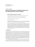
Figure 1: SVND algorithms make a nonlinear mapping from
the input space to the feature space. A simple geometric figure
(hypersphere or hyperplane) is traced therein, which splits the
feature space into known domain and unknown domain. This
corresponds to a nonlinear, complex geometry boundary in the
input space.
Note from (10) that hyperplane in F is given by a linear
combination of the mapped input vectors, and accordingly,
the patterns with α
i
/
=0arecalledSupport Vectors. They
contain all the relevant information for describing the
hyperplane in F that separates the data in the input space.
The number of support vector is usually small (i.e, SVM gives
a sparse solution), and it is related to the generalization error
of the classifier.
3.3. Kernel-Based One-Class Skin Segmentation. The domain
description of a multidimensional distribution can be
addressed by using kernel algorithms that systematically
enclose the data points into a nonlinear boundary in the
input space. SVND algorithms distinguish between the class
of objects represented in the training set and all the other
possible objects. It is important to highlight that SVND
represents a very different problem than the SVM. The

training of SVND only uses training samples from one
single class (skin pixels), whereas an SVM approach requires
training with pixels from two different classes (skin and
nonskin). Hence, let X
≡{x
1
, , x
l
} be now a set of l
observed only skin samples in a space color. Note that, in this
case, nonskin samples are not used in the training dataset.
Two main algorithms for SVND have been proposed,
that are based on different geometrical models in the feature
space, and their schematic is depicted in Figure 1.Oneof
them uses a maximum margin hyperplane in F that separates
the mapped data from the origin of F [18], whereas the other
finds a hypersphere in F with minimum radius enclosing the
mapped data [19]. These algorithms are next summarized.
3.3.1. SVND with Hyperplane. The SVND algorithm pro-
posedin[18] builds a domain function whose value is
+1 in the half region of F that captures most of the data
points, and
−1 in the other half region. The criterion
followed therein consists of first mapping the data into F,
and then separating the mapped points from the origin with
maximum margin. This decision function is required to be
positive for most training vectors x
i
, and it is given by
f

(
x
)
= sgn

w, ϕ
(
x
)

−ρ

, (13)
where w, ρ, are the maximum margin hyperplane and the
bias, respectively. For a newly tested point x, decision value
f (x) is determined by mapping this point to F and then
evaluating to which side of the hyperplane it is mapped.
In order to state the problem, two terms are simultane-
ously considered. On the one hand, the maximum margin
condition can be introduced as usual in SVM classification
formulation [26], and then, maximizing the margin is
equivalent to minimizing the norm of the hyperplane vector
w. On the other hand, the domain description is required to
bound the space region that contains most of the observed
data, but slack variables ξ
i
are introduced in order to
consider some losses, that is, to allow a reduced number
of exceptional samples outside the domain description.
Therefore, the optimization criterion can be expressed as the

simultaneous minimization of these two terms, that is, we
want to minimize
1
2
w
2
+
1
νl
l

i=1
ξ
i
−ρ, (14)
with respect to w, ρ andconstrainedto

w, ϕ
(
x
i
)

≥
ρ −ξ
i
, (15)
and to ρ>0, and to ξ
i
≥ 0, for i = 1, , l. Parameter

ν
∈ (0, 1) is introduced to control the tradeoff between the
margin and the losses.
The Lagrangian functional can be stated, similarly to the
preceding subsection, and now, the dual problem reduces to
minimizing
1
2
l

i,j=1
α
i
α
j
K

x
i
, x
j

(16)
constrained to the KKT conditions given by

l
i=1
α
i
= 1, 0 ≤

α
i
≤ 1/νl,andw =

l
i
=1
α
i
ϕ(x
i
).
It can be easily shown that samples x
i
that are mapped
into the +1 semispace have no losses (ξ
i
= 0) and a null
coefficient α
i
, so that they are not support vectors. Also,
the samples x
i
that are mapped to the boundary have no
losses, but they are support vectors with 0 <α
i
< 1/νl,
and accordingly they are called unbounded support vectors.
Finally, samples x
i

that are mapped outside the domain
region have nonzero losses, ξ
i
> 0, their corresponding
Lagrange multipliers are α
i
= 1/νl, and they are called
bounded support vectors.
Solving this QP problem, the decision function (13)can
be easily rewritten as
f
(
x
)
= sgn
⎛
⎝
l

i=1
α
i
K
(
x, x
i
)
−ρ
⎞
⎠

. (17)
6 EURASIP Journal on Advances in Signal Processing
By now inspecting the KKT conditions, we can see that,
for ν close to 1, the solution consists of all α
i
being at
the (small) upper bound, which closely corresponds to a
thresholded Parzen window nonparametric estimator of the
density function of the data. However, for ν close to 0,
the upper boundary of the Lagrange multipliers increases
and more support vectors become then unbounded, so that
they are model weights that are adjusted for estimating the
domain that supports most of the data.
Bias value ρ can be recovered noting that any unbounded
support vector x
j
has zero losses, and then it fulfills.
l

i=1
α
i
K

x
j
, x
i

−

ρ = 0 =⇒ ρ =
l

i=1
α
i
K

x
j
, x
i

. (18)
It is convenient to average the value of ρ that is estimated
from all the unbounded support vectors, in order to reduce
the round-off error due to the tolerances of the QP solver
algorithm.
3.3.2. SVND with Hypersphere. The SVND algorithm pro-
posedin[19] follows an alternative geometric description of
the data domain. After the input training data are mapped
to feature space F, the smallest sphere of radius R,centered
at a
∈ F, is built under the condition that encloses most of
the mapped data inside it. Soft constrains can be considered
by introducing slack variables or losses, ξ
i
≥ 0, in order to
allow a small number of atypical samples being outside the
domain sphere. Then the primal problem can be stated as

the minimization of
R
2
+ C
l

i=1
ξ
i
(19)
constrained to
ϕ(x
i
) − a
2
≤ R
2
+ ξ
i
for i = 1, , l,where
C is now the tradeoff parameter between radius and losses.
Similarly to the preceding subsections, by using the
Lagrange Theorem, the dual problem consists now of
maximizing
−
l

i,j=1
α
j

α
i
K

x
j
, x
i

+
l

i=1
α
i
K
(
x
i
, x
i
)
(20)
constrained to the KKT conditions, and where the α
i
are now
the Lagrange multipliers corresponding to the constrains.
The KKT conditions allow us to obtain the sphere center
in the feature space, a
=


l
i
=1
α
i
ϕ(x
i
), and then, the distance
of the image of a given point x to the center can be calculated
as
D
2
(
x
)
=


ϕ(x) −a


2
= K
(
x, x
)
−2
l


i=1
α
i
K
(
x
i
, x
)
+
l

i,j=1
α
i
α
j
K

x
i
, x
j

.
(21)
In this case, samples x
i
that are mapped strictly inside
the sphere have no losses and null coefficient α

i
,andare
not support vectors. Samples x
i
that are mapped to the
sphere boundary have no losses, and they are support vectors
with 0 <α
i
<C(unbounded support vectors). Samples
x
i
that are mapped outside the sphere have nonzero losses,
ξ
i
> 0, and their corresponding Lagrange multipliers are
α
i
= C (bounded support vectors). Therefore, the radius of
the sphere is the distance to the center in the feature space,
D(x
j
), for any support vector x
j
whose Lagrange multiplier
is different from 0 and from C, that is, if we denote by R
0
the
radius of the solution sphere, then
R
2

0
= D
2

x
j

(22)
The decision function for a new sample belonging to the
domain region is now given by
f
(
x
)
= sgn

D
2
(
x
)
−R
2
0

, (23)
which can be interpreted in a similar way to the SVND
with hyperplane. A difference now is that a lower value of
the decision statistic (distance to the hypersphere center)
is associated with the skin domain, whereas in SVND with

hyperplane, a higher value for the statistic (distance to the
coordenate hyperorigin) is associated with the skin domain.
4. Experiments and Results
In this section, experiments are presented in order to deter-
mine the accuracy of conventional and kernel methods for
skin segmentation. According to our application constraints,
the experimental setting considered two main characteristics
of the data, namely, the importance of controlled lighting
and acquisition conditions, which was taken into account
by using two different databases described next, and the
consideration of three different chromaticity color spaces.
In these situations, we analyzed the performance of two
conventional skin detectors (GMM and MLP), and three
kernel methods (binary SVM, and one-class hyperplane and
hypersphere SVND algorithms).
4.1. Experiments and Results. As pointed out in Section 2,
one of the main aspects to consider in the design of
the optimum skin detector for a specific application is
the lighting conditions. If lighting conditions (mainly its
spectral distribution) can be controlled, a chromaticity
space with intensity normalization will probably generalize
better than a 3D one when there is not enough variability
to represent the 3D color space. In order to tackle this
problem, we will consider a database of face images in an
office environment, acquired with several different webcams,
with the goal of building a face recognition application
for Internet services. With this setup, our restrictions are;
(i) mainly Caucasian people considered; (ii) a medium-
size labeled dataset available; (iii) office background and
mainly indoor lighting will be present (iv) webcams using the

automatic white balance correction (control of color spectral
distribution).
Databases. We considered using other available databases,
for instance, XM2VTS database [27] for controlled lighting
EURASIP Journal on Advances in Signal Processing 7
With GMM With MLP
With SVC With SVND−S
With GMM
With MLP
With SVC
With SVND−S
With GMM
With MLP
With SVC With SVND−S
With GMM With MLP
With SVC With SVND−S
(a0) (a1) (a2) (a3) (a4)
(b0) (b1) (b2) (b3) (b4)
(c0) (c1) (c2) (c3) (c4)
(d0) (d1) (d2) (d3) (d4)
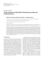
Figure 2: Examples of RGB images in the databases: (a0, b0) from CdB, and (c0, d0) from UdB. Classifiers correspond to GMM (∗1), MLP
(
∗2), SVM (∗3), and SVND-S (∗4). Nonskin pixels in black and skin pixels in white.
and background conditions dataset, but color was poorly
represented in these images due to video color compression.
With BANCA [28] for uncontrolled lighting and background
conditions dataset, we found the same restrictions. There-
fore, we assembled our own databases.
First, a controlled dataBase (from now, CdB)of224
face images from 43 different Caucasian people (examples

in Figure 2(a0, b0)) was assembled. Images were acquired
by the same webcam in the same place under controlled
lighting conditions. The webcam was configured to output
linear RGB with 8 bits per channel in snapshot mode. This
database was used to evaluate the segmentation performance
under controlled and uniform conditions.
Second, an uncontrolled dataBase (from now, UdB)
of 129 face images from 13 different Caucasian people
(examples in Figure 2(c0, d0)) was assembled. Images were
taken from eight different webcams in automatic white
balance configuration, in manual or automatic gain control,
and under differently mixed lighting sources (tungsten,
fluorescent, daylight). This database was used to evaluate
the robustness of the detection methods under uncontrolled
light intensity but similar spectral distribution.
For both databases, around half million skin and nonskin
pixels were selected manually from RGB images.
Color Spaces. The pixels in the databases were subsequently
labeled and transformed into the next color spaces.
(i) YCbCr, a color-difference coding space defined for
digital video by the ITU. We used the recommenda-
tion ITU-R BT.601-4, that can be easily computed as
an offset linear transformation of RGB.
(ii) CIEL
∗
a
∗
b
∗
, a colorimetric and perceptually uniform

color space defined by the Commission Internationale
de L’Eclairage, nonlinearly and quite complexly
related to RGB.
(iii) normalized RGB, an easy nonparametriclinear trans-
formation of RGB that normalizes every RGB chan-
nel by their sum, so that r + g + b
= 1.
Chrominance components of skin color in these spaces
were assumed to be only slightly dependent on the luminance
component (decreasingly dependent in YCbCr, CIEL
∗
a
∗
b
∗
,
and normalized RGB) [29, 30]. Hence, in order to reduce
8 EURASIP Journal on Advances in Signal Processing
0.8
0.7
0.6
0.5
0.4
0.3
Cr
0.30.40.50.60.70.8
Cb
(a)
0.6
0.4

0.2
0
−0.2
−0.4
b
∗
−0.4 −0.20 0.20.40.6
a
∗
(b)
0.6
0.5
0.4
0.3
0.2
0.1
g
0.10.20.30.40.50.60.70.8
r
(c)
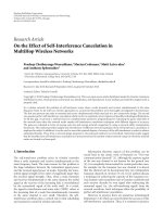
Figure 3: CdB skin (red) and nonskin (gray) samples used for test: (a) in CbCr space; (b) in a
∗
b
∗
components CIEL
∗
a
∗
b
∗

space; (c) in rg
component from normalized RGB.
domain and distribution dimensionality, only 2D spaces
were considered, and they were CbCr components in YCbCr,
a
∗
b
∗
components in CIEL
∗
a
∗
b
∗
, and rg components in
normalized RGB. Figure 3 shows the resulting data for pixels
in CdB.
4.2. Experiments and Results. For each segmentation proce-
dure, the Half Total Error Rate (HTER) was measured for
featuring the performance provided by the method, that is,
HTER
=
FAR + FRR
2
×100 (24)
where FAR and FRR are False Acceptance and False Rejection
Ratios, respectively, measured at the Equal Error Rate (EER)
point, that is, in the point where the proportion of false
acceptances is equal to the proportion of false rejections.
Usually, the performance of a system is given over a test set

and the working point is chosen over the training set. In this
work we give the FAR, FRR and HTER figures for a system
working in the EER point set in training.
The model complexity (MC) was also obtained as a figure
of merit for the segmentation method, given by the number
of Gaussian components in GMM, by the number of neurons
in the hidden layer in MLP, and by the percentage of support
vectors in kernel-based detectors, that is, MC
= #sv/l ×100,
where #sv is the number of support vectors (α
i
> 0) and l is
the number of training samples.
The tuning set for adjusting the decision threshold
consisted of the skin samples and the same amount of
nonskin samples. Performance was evaluated in a disjoint set
(test set) which included labeled skin and nonskin pixels.
4.3. Results with Conventional Segmentation. We us ed GM M
as the base procedure to compare with due to it has
been commonly used in color image processing for skin
applications. Here, we used 90 000 skin samples to train the
model, 180 000 non-skin and skin samples (the previous
90 000 skin samples plus other 90 000 non-skin samples) to
adjust the threshold value, and new 250 000 samples (170 000
of nonskin and 80 000 of skin) to test the model.
Table 1: HTER values for GMM at EER working point with
increasing number of mixtures.
k
13579
CdB

CbCr 11.5 11.9 12.9 12.8 12.9
a
∗
b
∗
7.5 8.6 8.7 8.7 9.0
rg 7.3 7.8 7.7 9.0 8.1
UdB
CbCr 24.1 25.6 25.1 25.5 23.9
a
∗
b
∗
23.6 26.1 22.3 24.0 24.5
rg 22.8 25.5 21.5 22.8 23.3
Ta ble 1 shows the HTER values for the three color spaces
and the two databases considered with different number
of Gaussian components (i.e, the model order) for the
GMM model. The model with a single Gaussian yielded
the minimum average error in segmentation when images
were taken under controlled lighting conditions (CbB), but
under uncontrolled lighting conditions (UdB) the optimum
number of Gaussians was quite noisy for our dataset. As
could be expected, results were better for pixel classification
under controlled lighting conditions, below 12% of HTER in
all model orders. Performance decreased under uncontrolled
lighting conditions, showing values of HTER over 20% in the
three color spaces.
Ta ble 2 shows the results for GMM trained with different
number of skin samples. In both databases (controlled and

uncontrolled acquisition conditions) the performance in
CbCr, a

b

and rg color spaces is similar. Nevertheless,
performance for UdB was worse than for CdB. It can
be seen that under controlled acquisition conditions the
results obtained for the three color spaces showed the lowest
HTER for
= 1. Therefore, under controlled image capturing
conditions, there was no apparent gain in using a more
sophisticated model, and this result is coherent with the
reported in [2]. By the values obtained for GMM under
uncontrolled acquisition conditions, we can conclude that
there is not a fix value of k which offers statistically significant
better results.
EURASIP Journal on Advances in Signal Processing 9
Table 2: HTER values for GMM at EER working point with
different number of skin training samples.
GMM GMM
250 samples 90000 samples
FAR–FRR HTER k FAR–FRR HTER k
CdB
CbCr 7.8–14.7 11.3 1 12.0–11.0 11.5 1
a
∗
b
∗
4.2–10.0 7.1 1 7.5–7.4 7.5 1

rg 5.9–8.8 7.4 1 7.3–7.4 7.3 1
UdB
CbCr 18.1–29.0 23.6 1 24.0–23.8 23.9 9
a
∗
b
∗
17.9–27.2 22.6 7 22.5–22.2 22.3 5
rg 21.9–21.8 21.8 1 21.6–21.4 21.5 5
Table 3: HTER values for MLP at EER working point.
MLP
FAR–FRR HTER n
CdB
CbCr 7.5–9.7 8.6 20
a
∗
b
∗
5.3–5.7 5.5 5
rg 6.8–5.9 6.3 15
UdB
CbCr 9.5–13.1 11.3 10
a
∗
b
∗
11.0–13.3 12.1 10
rg 7.6–15.6 11.6 5
When the number of samples used for adjusting the
GMM model decreases from 90,000 to 250 (the same number

used for training the SVM models), the performance in terms
of HTER is similar, but the EER threshold (that uses non skin
samples) was clearly more robust if more samples were used
to estimate it, that is, by using 250 samples, the difficulty of
generalizing an EER point increases. For example, in CbCr
color space, FAR
= 18.1,FRR = 29.0 by using 250 samples
and FAR
= 24.0, FRR = 23.8 with 90,000 samples.
Ta ble 3 shows the results for MLP with one hidden layer
and n hidden neurons. Similarly to GMM, performance for
CdB is better than for UdB in the three color spaces, but
the network complexity, measured as the optimal number
of hidden neurons, is higher in CbCr and rg for CdB
than for UdB. Therefore, under light intensity uncontrolled
conditions, the performance does not improve by using more
complex networks. Moreover, note that each color space
in each database requires a different network complexity.
Comparing the values of HTER with the corresponding
ones obtained with GMM, MLP is superior to GMM in
all considered cases. This improvement is even higher for
UdB.
4.4. Results with Kernel-Based Segmentation. As described in
Section 2, an SVM and two SVND algorithms (SVND-H
and SVND-S) have been considered. For all of them, model
tuning must be first addressed, and the free parameters of the
model (
{C, σ} in SVM and SVND-S, and {ν, σ} in SVND-
H) have to be properly tuned. Recall that both C and ν are
introduced to balance the margin and the losses in their

respective problems, whereas σ represents in both cases the
width of the Gaussian kernel. Therefore, these parameters are
expected to be dependent on the training data.
The training and the test subsets were obtained from two
main considerations. First, although the SVMs can be trained
with large and high-dimensional training sets, it is also
well known that the computational cost increases when the
optimal model parameters are obtained by using the classical
Quadratic Programing as optimization method. And second,
the SVMs methods have shown a good generalization
capability for a lot of different problems previously in
literature. Due to both reasons, a total of only 250 skin
samples were randomly picked (from the GMM training set)
for the two SVND algorithms, and a total of only 500 samples
(the previous 250 skin samples plus 250 non-skin samples
randomly picked from the GMM tuning set) for the SVM
model.
After considering enough wide ranges to ensure that both
optimal free parameters of each SVM model (
{C, σ} for
SVND-S and SVM;
{ν, σ} for SVND-H) can be obtained, we
found that with SVND-S,
{C = 0.5, σ = 0.05} were selected
as the optimal values of the free parameters for the three
color spaces and CdB database, and
{C = 0.05, σ = 0.1} for
the three color spaces and UdB database; with SVND-H, the
most appropiate values for the three color spaces were
{ν =

0.01, σ = 0.05} for CdB database, and {ν = 0.08, σ = 0.2} for
UdB; and with SVM, the optimal values for all color spaces
were
{C = 46.4, σ = 1.5} for CdB and {C = 215.4, σ = 2.5}
for UdB.
Ta ble 4 shows the detailed results for three kernel
methods: SVND-H, SVND-S, and SVM, with their free
parameters. The performance obtained with both SVND
methods is very similar, as HTER and MC values are very
close for the same color space and the same database.
Although the lowest values of HTER are achieved with SVM
in all the cases, the improvement is even higher for UdB.
For example, in rg color space and CdB, HTER
= 5.8with
SVM versus HTER
= 6.4 with SVDN mehods, while for UdB,
HTER
= 10.8 with SVM and HTER > 13 with SVDN. When
we focus on the performance in terms of EER threshold, the
behaviour of SVND methods shows more robustness, that
is, the FAR and FRR values are closer than those achieved
with SVM. Moreover, although the SVM gets the lowest
HTER values for Cdb and UdB, the required complexity
for UdB, measured in terms of MC values, is higher than
the corresponding one required by SVND methods (from
MC
= 23.6 with SVM to MC = 5.6 with SVND-S and
SVND-H).
4.5. Comparison of Methods. As an example, Figure 4 shows
the training samples and boundaries obtained with nonpara-

metric detectors (SVND-H, SVND-S, SVM, and MLP), and
for the three color spaces and both databases (CdB and UdB).
Note that in the two SVND algorithms, the boundaries in
terms of EER, obtained with the tuning set, were very close to
those given by the algorithm boundary: R
0
for SVND-S and
ρ
0
for SVND-H. Accordingly, a good first estimation of the
EER boundary can be done just by considering only the skin
samples of the training set, thus avoiding the selection of an
EER threshold over a tuning set. Therefore, no subset of non-
skin samples is needed with SVND for building a complete
10 EURASIP Journal on Advances in Signal Processing
SVND-H-CdB-CbCr
0.3
0.35 0.4 0.45 0.5 0.55 0.6
0.4
0.45
0.5
0.55
0.6
0.65
SVND-S-CdB-CbCr SVC-CdB-CbCr MLP-CdB-CbCr
–0.2 –0.1 0 0.1 0.2 0.3
–0.1
–0.05
0
0.05

0.1
0.15
0.2
0.25
0.3
0.35
0.4
SVND-H-CdB-rg
0.25 0.3 0.35 0.4 0.45 0.5 0.55
0.2
0.25
0.3
0.35
0.4
0.45
0.5
SVND-S-CdB-rg SVC-CdB-rg MLP-CdB-rg
SVND-H-UdB-CbCr SVND-S-UdB-CbCr SVC-UdB-CbCr MLP-UdB-CbCr
SVND-H-UdB-rg SVND-S-UdB-rg SVC-UdB-rg MLP-UdB-rg
(a0) (a1) (a2) (a3)
(b0) (b1) (b2) (b3)
(c0) (c1) (c2) (c3)
(d0) (d1) (d2) (d3)
(e0) (e1) (e2) (e3)
(f0) (f1) (f2) (f3)
0.3
0.35 0.4 0.45 0.5 0.55 0.6
0.4
0.45
0.5

0.55
0.6
0.65
0.3
0.35 0.4 0.45 0.5 0.55 0.6
0.4
0.45
0.5
0.55
0.6
0.65
0.3
0.35 0.4 0.45 0.5 0.55 0.6
0.4
0.45
0.5
0.55
0.6
0.65
0.3
0.35 0.4 0.45 0.5 0.55 0.6
0.4
0.45
0.5
0.55
0.6
0.65
0.3
0.35 0.4 0.45 0.5 0.55 0.6
0.4

0.45
0.5
0.55
0.6
0.65
0.3
0.35 0.4 0.45 0.5 0.55 0.6
0.4
0.45
0.5
0.55
0.6
0.65
–0.2 –0.1 0 0.1 0.2 0.3
–0.1
–0.05
0
0.05
0.1
0.15
0.2
0.25
0.3
0.35
0.4
–0.2 –0.1 0 0.1 0.2 0.3
–0.1
–0.05
0
0.05

0.1
0.15
0.2
0.25
0.3
0.35
0.4
–0.2 –0.1 0 0.1 0.2 0.3
–0.1
–0.05
0
0.05
0.1
0.15
0.2
0.25
0.3
0.35
0.4
–0.2 –0.1 0 0.1 0.2 0.3
–0.1
–0.05
0
0.05
0.1
0.15
0.2
0.25
0.3
0.35

0.4
–0.2 –0.1 0 0.1 0.2 0.3
–0.1
–0.05
0
0.05
0.1
0.15
0.2
0.25
0.3
0.35
0.4
–0.2 –0.1 0 0.1 0.2 0.3
–0.1
–0.05
0
0.05
0.1
0.15
0.2
0.25
0.3
0.35
0.4
0.25 0.3 0.35 0.4 0.45 0.5 0.55
0.2
0.25
0.3
0.35

0.4
0.45
0.5
0.25 0.3 0.35 0.4 0.45 0.5 0.55
0.2
0.25
0.3
0.35
0.4
0.45
0.5
0.25 0.3 0.35 0.4 0.45 0.5 0.55
0.2
0.25
0.3
0.35
0.4
0.45
0.5
0.25 0.3 0.35 0.4 0.45 0.5 0.55
0.2
0.25
0.3
0.35
0.4
0.45
0.5
0.25 0.3 0.35 0.4 0.45 0.5 0.55
0.2
0.25

0.3
0.35
0.4
0.45
0.5
0.25 0.3 0.35 0.4 0.45 0.5 0.55
0.2
0.25
0.3
0.35
0.4
0.45
0.5
0.3
0.35 0.4 0.45 0.5 0.55 0.6
0.4
0.45
0.5
0.55
0.6
0.65
–0.2 –0.1 0 0.1 0.2 0.3
–0.1
–0.05
0
0.05
0.1
0.15
0.2
0.25

0.3
0.35
0.4
0.25 0.3 0.35 0.4 0.45 0.5 0.55
0.2
0.25
0.3
0.35
0.4
0.45
0.5
SVND-H-CdB-a
∗
b
∗
SVND-S-CdB-a
∗
b
∗
SVC-CdB-a
∗
b
∗
MLP-CdB-a
∗
b
∗
SVND-H-UdB-a
∗
b

∗
SVND-S-UdB-a
∗
b
∗
SVC-UdB-a
∗
b
∗
MLP-UdB-a
∗
b
∗
Figure 4: Training samples (skin in red, nonskin in green) and skin boundaries (continuous for SVND threshold, dashed for EER threshold),
obtained from the nonparametric models (each column corresponds to a model: SVND-H in
∗0, SVND-S in ∗1, SVM in ∗2, and MLP in
∗3). CdB with CbCr in a∗, CdB with a

b

in b∗, CdB with rg in c∗, UdB with CbCr in d∗, UdB with a

b

in e∗, UdB with rg in f ∗.
EURASIP Journal on Advances in Signal Processing 11
Table 4: Values of HTER (%) and complexity for SVND-H (nu = 0.01, σ = 0.05 for CdB; nu = 0.08, σ = 0.2forUdB),SVND-S(C = 0.5,
σ
= 0.05 for CdB; C = 0.05, σ = 0.1forUdB)andSVM(C = 46.4, σ = 1.5forCdB;C = 215.4, σ = 2.5forUdB).
SVND-H SVND-S SVM

FAR–FRR HTER ρ
0
MC FAR–FRR HTER R
0
MC FAR–FRR HTER MC
CdB
CbCr 8.7–8.7 8.7 11.7 40.4 8.4–8.2 8.8 25.1 50.4 7.9–8.3 8.1 17.2
a
∗
b
∗
7.6–7.6 7.6 7.5 40.4 7.6–7.6 7.6 26.6 51.2 3.9–6.7 5.3 19.0
rg 6.4–6.4 6.4 21.5 40.4 6.4–6.4 6.4 25.0 50.4 5.1–6.5 5.8 17.4
UdB
CbCr 16.2–16.2 16.2 19.1 5.6 13.4–13.4 13.4 25.2 1.6 7.7–13.7 10.7 22.4
a
∗
b
∗
15.9–15.9 15.9 40.9 5.6 14.3–17.4 15.9 19.2 5.6 9.1–16.0 12.5 19.8
rg 13.3–13.3 13.3 18.1 5.6 13.2–13.2 13.2 15.3 5.6 7.2–14.4 10.8 23.6
Table 5: All values of HTER (%).
SVND-H SVND-S SVM MLP GMM
CdB
CbCr 8.7 8.8 8.1 8.6 11.3
a
∗
b
∗
7.6 7.6 5.3 5.5 7.1

rg 6.4 6.4 5.8 6.3 7.4
UdB
CbCr 16.2 13.4 10.7 11.3 23.6
a
∗
b
∗
15.9 15.9 12.5 12.1 22.6
rg 13.3 13.2 10.8 11.6 21.8
Table 6: HTER values at EER for two-class SVM and 3D color
spaces.
SVM
FAR–FRR HTER MC
CdB
YCbCr 6.7–4.9 5.8 16
CIEL
∗
a
∗
b
∗
4.6–6.7 5.6 22
rgb 5.8–6.7 6.2 19
UdB
YCbCr 6.9–21.5 14.2 24.8
CIEL
∗
a
∗
b

∗
7.0–23.5 15.2 23.2
rgb 7.4–14.3 10.8 25.6
skin detector, though the use of a test set with samples
from both classes can be useful for a subsequent security
verification of the threshold provided by the algorithm.
Nevertheless, due to the extremely high density of samples
near the decision boundaries, those nonparametric models
trained with skin and non-skin samples are able to yield
more complex and accurate boundaries, whereas models
trained with only skin samples yield a good skin domain
description at the expense of increased skin and non-skin
samples overlapping. The effect of the boundary estimation
on the segmentation can be seen in Figure 4, which shows
several representative examples of the pixel-classified images
in CdB and UdB by using the analyzed detectors.
A summary of the performance obtained by the five dif-
ferent classifier (in terms of HTER over the test data set) can
be found in Ta b le 5 . We can conclude that, under controlled
image acquisition conditions, nonparametric methods yield
higher accuracy than GMM. The difference is even higher
under uncontrolled capturing conditions. For example, with
a

b

color space in UdB, HTER = 22.6forGMMversus
HTER
= 15.9 for SVND-H (in this case, the worse of
the three SVM-based methods considered). It is interesting

to emphasize that both SVND models can be also seen as
isotropic Gaussian mixtures (see (17) and (27)), with the
important difference that SVND training puts the centers
of Gaussian kernels at samples (support vectors) that are
more relevant for describing the domain of interest. We must
remark also that SVM-based segmentation algorithms are
nonparametric methods which obtain the required MC from
the available data, thus avoiding searches like the number
of components in GMM. When comparing kernel-based
methods with MLP, the last one shows lower HTER values
than GMM and SVNN for most of the color spaces, but
always higher than the corresponding ones of SVM (the
differences are significant according to a paired-sample T-
test). Therefore, the MLP can be considered as an alternative
to SVDN methods, but not to SVM. Moreover, MLP has
the problem of finding local minimum solutions, while SVM
always finds the global minimum.
With respect to the SVM-based methods, we can con-
clude that the best performance, in terms of HTER, is
provided by the standard SVM classifier for all the color
spaces and databases studied. Hence, when the goal of the
application under study is the skin segmentation, this is a
more appropriate approach to be considered. However, when
it is pursued to obtain an adequate description of the domain
that represents the support for skin pixels in the color
space, rather than its statistical density descriptions, the best
solution is to use an SVND algorithm. Moreover, with SVND
algorithms, R
0
and ρ

0
values can be considered as default
decision statistics or thresholds, for SVND-S and SVND-H,
respectively, while for GMM and SVM the decision statistic
must be set a posteriori and non-skin samples are required.
4.6. Two-Class SVM and 3D Color Spaces. As we mentioned
in Section 2.1, we have constrained our experiments to
the application cases where not enough 3D labeled data is
available for an accurate modeling of the 3D color space. In
order to show that the skin segmentation performs better
in this application if only 2D color spaces are considered,
we have obtained the performance for the two-class SVM
classifier (the best of the five considered for 2D color spaces)
in the three different 3D color spaces and the two databases,
by considering the same conditions (500 training samples).
The obtained results are shown in Ta ble 6 , which shows that
the HTER values are higher than the corresponding ones
obtained by using only 2D spaces, except for YCbCr-CdB
(see Ta b le 4 ). Moreover, the differences are higher under
uncontrolled lighting conditions.
12 EURASIP Journal on Advances in Signal Processing
5. Conclusions
We have presented a comparative study between pixel-wise
skin color detection using GMM, MLP and a three different
kernel-based methods: the classical SVM, and two one-
class methods (SVND) on three different chromaticity color
spaces. All kernel-based models studied have shown some
interesting advantages for skin detection applications when
compared to GMM and MLP. Moreover, each SVM-based
method solves a QP problem, which has a unique solution,

and hence there is no randomness in the initialization
settings. When the main interest of the application is an
adequate description of the skin pixel domain, the SVND
approaches have shown to be more adequate than those
based on modeling probability density function. However,
when the objective is the skin detection, which is a more
usual application in practice, the classical SVM outper-
formed the SVND ones in terms of HTER for the three
color spaces and the two different databases (under con-
trolled and specially under uncontrolled lighting conditions)
considered, due to its use of the boundary information from
skin and non-skin samples during its design. Our aim was to
focus on two characteristics of the broad skin segmentation
problem, namely, the importance of controlled lighting and
acquisition conditions, and the influence of the chromaticity
color spaces. In this work we have created our dataset with
only caucasian people; the extension to schemes dealing with
other-skin tones is one of the main related future research
issues.
Acknowlegment
This work has been partially supported by Research Projects
TEC2007-68096-C02/TCM and TEC2008-05894 from Span-
ish Government.
References
[1] J. Cai, A. Goshtasby, and C. Yu, “Detecting human faces in
color images,” Image a nd Vision Computing,vol.18,no.1,pp.
63–75, 1999.
[2] R L. Hsu, M. Abdel-Mottaleb, and A. K. Jain, “Face detection
in color images,” IEEE Transactions on Pattern Analysis and
Machine Intelligence, vol. 24, no. 5, pp. 696–706, 2002.

[3] M. H. Yang and N. Ahuja, “Extracting gestural motion trajec-
tory,” in Proceedings of the 3rd IEEE International Conference
on Automat ic Face and Gesture Recognition, 1998.
[4] K K. Sung and T. Poggio, “Example-based learning for view-
based human face detection,” IEEE Transactions on Patte rn
Analysis and Machine Intelligence, vol. 20, no. 1, pp. 39–51,
1998.
[5] Y. Li, A. Goshtasby, and O. Garcia, “Detecting and tracking
human faces in videos,” in Proceedings of the 15th IEEE
International Conference on Pattern Recognition (ICPR ’00),
vol. 1, pp. 807–810, 2000.
[6] M J. Chen, M C. Chi, C T. Hsu, and J W. Chen, “ROI video
coding based on H.263+ with robust skin-color detection
technique,” IEEE Transactions on Consumer Electronics, vol. 49,
no. 3, pp. 724–730, 2003.
[7] J. Brand and J. S. Mason, “A comparative assessment of
three approaches to pixel-level human skin-detection,” in
Proceedings of the 15th IEEE International Conference on
Pattern Recognition ((ICPR ’00), vol. 1, pp. 1056–1059, 2000.
[8] H. Wang and S F. Chang, “A highly efficient system for
automatic face region detection in MPEG video,” IEEE
Transactions on Circuits and Systems for Video Technology, vol.
7, no. 4, pp. 615–628, 1997.
[9] M H. Yang and N. Ahuja, “Detecting human faces in color
images,” in Proceedings of the IEEE International Conference on
Image Processing, vol. 1, pp. 127–130, 1998.
[10] J. C. Terrillon, M. N. Shirazi, H. Fukamachi, and S. Akamatsu,
“Comparative performance of different skin chrominance
models and chrominance spaces for the automatic detection
of human faces in color images,” in Proceedings of the 5th

IEEE International Conference on Automatic Face and Gesture
Recognition, 2000.
[11] M H. Yang and N. Ahuja, “Gaussian mixture model for
humanskincoloranditsapplicationsinimageandvideo
databases,” in Conference on Storage and Retrieval for Image
and Video Databases, vol. 3656 of Proceedings of SPIE, pp. 458–
466, 1999.
[12] S. L. Phung, A. Bouzerdoum, and D. Chai, “Skin segmentation
using color pixel classification: analysis and comparison,” IEEE
Transactions on Pattern Analysis and Machine Intelligence, vol.
27, no. 1, pp. 148–154, 2005.
[13] M. J. Jones and J. M. Rehg, “Statistical color models with appli-
cation to skin detection,” International Journal of Computer
Vision, vol. 46, no. 1, pp. 81–96, 2002.
[14] H. Jin, Q. Liu, H. Lu, and X. Tong, “Face detection using one-
classSVMincolorimages,”inProceedings of the International
Conference on Signal Processing (ICSP ’04), pp. 1432–1435,
2004.
[15]R.N.Hota,V.Venkoparao,andS.Bedros,“Facedetection
by using skin color model based on one class classifier,” in
Proceedings of the 9th International Conference on Information
Technology (ICIT ’06), pp. 15–16, 2006.
[16] J C. Terrillon, M. N. Shirazi, M. Sadek, H. Fukamachi,
and T. S. Akamatsu, “Invariant face detection with support
vector machines,” in Proceedings of the 15th IEEE International
Conference on Pattern Recognition (ICPR ’00), 2000.
[17]Z.XuandM.Zhu,“Color-basedskindetection:surveyand
evaluation,” in Proceedings of the 12th International Multi-
Media Modelling Conference (MMM ’06), pp. 143–152, 2006.
[18] B. Sch

¨
olkopf, R. C. Williamson, A. J. Smola, J. Shawe-Taylor,
and J. Platt, “Support vector method for novelty detection,”
in Advances in Neural Information Processing Systems, vol. 12,
2000.
[19] D. M. J. Tax and R. P. W. Duin, “Support vector domain
description,” Pattern Recognition Letters, vol. 20, no. 11–13, pp.
1191–1199, 1999.
[20] B. D. Zarit, B. J. Super, and F. H. Queck, “Comparison of five
color models in skin pixel classification,” in Proceedings of the
International Workshop on Recognition, Analysis, and Tracking
of Faces and Gestures in Real-Time Systems, 1999.
[21] A. Albiol, L. Torres, and E. J. Delp, “Optimum color spaces
for skin detection,” in Proceedings of the IEEE International
Conference on Image Processing, vol. 1, pp. 122–124, 2001.
[22] S. Jayaram, S. Schmugge, M. C. Shin, and L. V. Tsap, “Effect of
colorspace transformation, the illuminance component, and
color modeling on skin detection,” in Proceedings of the IEEE
Computer Society Conference on Computer Vision and Pattern
Recognition (CVPR ’04), vol. 2, pp. 813–818, 2004.
EURASIP Journal on Advances in Signal Processing 13
[23] M. Soriano, B. Martinkauppi, S. Huovinen, and M. Laakso-
nen, “Adaptive skin color modeling using the skin locus for
selecting training pixels,” Pattern Recognition,vol.36,no.3,
pp. 681–690, 2003.
[24] A. Dempster, N. Laird, and D. Rubin, “Maximum likelihood
from incomplete data via the EM algorithm,” Journal of the
Royal Statistical Society, Series B, vol. 39, no. 1, pp. 1–38, 1997.
[25] G. Camps-Valls, J. L. Rojo-
´

Alvarez, and M. Mart
´
ınez-Ram
´
on,
Kernel Methods in Bioengineer ing, Communications and Image
Processing, IDEA Group, 2006.
[26] V. Vapnik, Statistical Learning Theor y, John Wiley & Sons, New
York, NY, USA, 1998.
[27] K. Messer, J. Matas, J. Kittler, J. Luettin, and G. Maitre,
“Xm2vtsdb: the extended m2vts database,” in Proceedings
of the Internat ional Conference on Audioand Video-Based
Biometric Person Authentication (AVBPA ’99), 1999.
[28] E. Bailly-Bailli
´
ere, S. Bengio, F. Bimbot, et al., “The BANCA
database and evaluation protocol,” in Proceedings of the 4th
International Conference on Audioand Video-Based Biometric
Person Authentication (AVBPA ’03), pp. 625–638, 2003.
[29] B. Menser and M. Brunig, “Locating human faces in color
images with complex background,” in Proceedings of the IEEE
International Symposium on Intelligent Signal Processing and
Communication Systems (ISPACS ’99), pp. 533–536, 1999.
[30] K. Sobottka and I. Pitas, “A novel method for automatic face
segmentation, facial feature extraction and tracking,” Signal
Processing: Image Communication, vol. 12, no. 3, pp. 263–281,
1998.