báo cáo hóa học:" Research Article Using a State-Space Model and Location Analysis to Infer Time-Delayed Regulatory Networks" potx

Hindawi Publishing Corporation
EURASIP Journal on Bioinformatics and Systems Biology
Volume 2009, Article ID 484601, 14 pages
doi:10.1155/2009/484601
Research Article
Using a State-Space Model and Location Analysis to
Infer Time-Delayed Regulatory Networks
Chushin Koh,
1
Fang-Xiang Wu,
2, 3
Gopalan Selvaraj,
4
and Anthony J. Kusalik
1, 3
1
Department of Computer Science, University of Saskatchewan, Saskatoon, SK, Canada S7N 5C9
2
Department of Mechanical Engineering, University of Saskatchewan, Saskatoon, SK, Canada S7N 5A9
3
Division of Biomedical Engineering, University of Saskatchewan, Saskatoon, SK, Canada S7N 5A9
4
Plant Biotechnology Institute, National Research Council of Canada, Saskatoon, SK, Canada S7N 0W9
Correspondence should be addressed to Anthony J. Kusalik,
Received 31 January 2009; Revised 4 May 2009; Accepted 15 July 2009
Recommended by Seungchan Kim
Computational gene regulation models provide a means for scientists to draw biological inferences from time-course gene
expression data. Based on the state-space approach, we developed a new modeling tool for inferring gene regulatory networks,
called time-delayed Gene Regulatory Networks (tdGRNs). tdGRN takes time-delayed regulatory relationships into consideration
when developing the model. In a ddition, a priori biological knowledge from genome-wide location analysis is incorporated into
the structure of the gene regulatory network. tdGRN is evaluated on both an artificial dataset and a published gene expression

data set. It not only determines regulatory relationships that are known to exist but also uncovers potential new ones. The results
indicate that the proposed tool is effective in inferring gene regulatory relationships with time delay. tdGRN is complementary to
existing methods for inferring gene regulatory networks. T he novel part of the proposed tool is that it is able to infer time-delayed
regulatory relationships.
Copyright © 2009 Chushin Koh et al. This is an open access article distributed under the Creative Commons Attribution License,
which permits unrestricted use, distribution, and reproduction in any medium, provided the original work is properly cited.
1. Introduction
Microarray technology allows researchers to study expression
profiles of thousands of genes simultaneously. One of the
ultimate goals for measuring expression data is to reverse
engineer the internal structure and function of a transcrip-
tional regulation network that governs, for example, the
development of an organism, or the response of the organism
to the changes in the external environment. Some of these
investigations also entail measurement of gene expression
over a time course after per turbing the organism. This is
usually achieved by measuring changes in gene expression
levels over time in response to an initial stimulation such
as environmental pressure or drug addition. The data
collected from time-course experiments are subjected to
cluster analysis to identify patterns of expression triggered
by the per turbation [1, 2]. A fundamental assumption is
that genes sharing similar expression patterns are commonly
regulated, and that the genes are involved in related biological
functions. Biologists refer to this as “guilt by association.”
Some frequently used clustering methods for finding coreg-
ulated genes are hierarchical clustering, trajectory clustering,
k-means clustering, principal component analysis (PCA),
and self-organizing maps (SOMs). A general review of these
clustering techniques is presented by Belacel et al. [3].

A gene network derived by the above clustering methods
is often represented as a wiring diagram. Cluster analysis
groups genes with similar time-based expression patterns
(i.e., trajectories) and infers shared regulatory control of
the genes. The clustering result allows one to find the
part-to-part correspondences between genes. The extents of
gene-gene interactions are captured by heuristic distances
generated by the analysis. The network diagram produced
provides insights into the underlying molecular interaction
network structure.
Two major limitations of conventional clustering meth-
ods are that (1) they cannot capture the effects of regulatory
genes that are not included in the microarray; (2) they
do not account for transcriptional time delay which occurs
in cells. For example, transcription of a gene depends on
2 EURASIP Journal on Bioinformatics and Systems Biology
the assembly of a transcribing complex, and that complex
typically contains several proteins. Some of these are core
proteins that catalyze mRNA synthesis and others are factors
that modulate mRNA synthesis according to the genetic and
environmental specifications for a given gene. Consequently,
transcription of such genes is delayed due to the time needed
for the production and assembly of the corresponding
transcr iption factors and their assembly into a transcription-
competent complex. An example of this is p53 and mdm2 as
discussed by Bar-Or et al. [4] where over-expression of p53
triggers a negative feedback mechanism. First, p53 stimulates
expression of the mdm2 gene. The production of mdm2
protein in turn represses the transcriptional functions of
p53 and promotes p53 proteolytic degradation [5]. Under

stress conditions, p53 and mdm2 proteins undergo damped
oscillations where mdm2 peaks with a delay of about
60 minutes relative to p53 [4]. In another example Ota
et al. [6] conducted a comprehensive analysis of delay in
transcriptional regulation using gene expression profiles in
yeast.
Wu et al. [7] propose the state-space approach to
model gene regulatory networks. Their research results have
shown that a state-space model can grasp a number of
properties of real-life gene regulatory networks. Recently,
Hu et al. [8] compared state-space models, fuzzy logical
models, and Baysian network models for gene regulatory
networks. Rangel et al. [9, 10] apply state-space modeling
to T-cell activation data. The technique provides a means
for constructing reliable gene regulatory networks based on
bootstrap statistical analysis. The method is applied to highly
replicated data. The confidence intervals of gene-gene inter-
action matrix elements are estimated by resampling with
replacement as many as 200 times. This approach, however,
has a severe limitation for application to microarray data
because most currently available time-course microarray
data are either replicated over only a few time points (<5)
or not replicated at all.
The above state-space models [7–10]donottaketime
delay in gene regulatory networks into consideration. How-
ever, examination of microarray data reveals a considerable
number of time delayed interactions, suggesting that time
delayisubiquitousingeneregulation[11]. From a biological
viewpoint, time delay in gene regulation arises from the
delays characterizing the various underlying processes such

as transcription, translation, and transport. For example,
time delays in regulation may stem from the time taken for
the transport of a regulatory protein to its site of action.
Recently, state-space models with time delays have
been proposed to account for the effects of missing data
and complex time delay relationships. In earlier work we
developed a state-space model with time delay to model yeast
cell-cycle data [12], and the model was demonstrated on
nonreplicated data. Our previous method [12] emphasized
identification of a set of internal state variables that govern
the cell-cycle process. It assumed that one gene does not
directly regulate another and thus does not partition the data
set. The drawbacks of this technique are that it is not clear
how a network can be derived from the modeling tool, and it
is hard to validate the model against biological knowledge of
time delay effects. In the same vein, Sung et al. [13]presented
a discretized Bayesian network model to construct a multiple
time delay gene network using the same data set. The Sung
et al. method focused on finding regulatory relationships
and associating the regulatory time delay with every “parent-
child” (i.e., regulator-target) pair [13]. The data set was
partitioned into parent set (the regulators) and child set
(the targets). The method suggested a new network structure
learning algorithm, Learning By Modification (LBM), to
identify potential regulators and then associate them with
target genes.
These existing state-space modeling techniques do not
incorporate the structure of gene regulatory networks
derived from biological knowledge. Alternatively, Li et al.
[14] have published their work on inferring transcription

factor activities using a discretized state-space modeling
technique. The Li et al. approach incorporates the results of
ChIP-on-chip (genome wide location analysis) experiments
into the model building. The network structure is predeter-
mined on the basis of a given transcription factor binding
to various gene probes in chromatin immuno-precipitation
(ChIP)-on-chip assays. The transcription factor activities are
then inferred with mathematical modeling using time-course
experiments. However, the Li et al. technique does not take
time delay into account.
To complement these existing methods, we have devel-
oped a new modeling tool called tdGRN for inferring
time delayed gene regulatory networks. tdGRN generates
a state space-based model into which time delays and the
ChIP-on-chip data are incorporated to infer a biologically
more meaningful network. A more extensive treatment of
tdGRN and the use of state-space model ling with time-series
microarray data can be found in the thesis of Koh [15].
2. Methodology
The tdGRN approach consists of three parts. First, we
implement a state-space model which incorporates multiple
time delays. Secondly, we incorporate ChIP-on-chip data for
determining network connectivity for both nonreplicated
and replicated data. This involves replacing Rangel’s boot-
strap confidence intervals (derived from highly replicated
data) for identifying gene-gene interaction with a substitute.
Finally, the networks generated from the new model are
visualized using techniques from the literature [16].
2.1. Time Delay Model. We consider the expression profile of
a regulator (e.g., a transcription factor) as an input function

to the system. Therefore, the time period, τ, from the over-
expression of the regulator to the over- or under-expression
of the targeted gene is represented as an input-delay function.
A gene regulatory system with p regulators, q target genes,
and n state variables can be described using the following
state-space model with time delays:
z
t+1
= Az
t
+ Bu
t−τ
+ w
t
,
x
t
= Cz
t
+ v
t
,
(1)
EURASIP Journal on Bioinformatics and Systems Biology 3
z
t
t
z
t+1
A

B
C
. . .
. . .
x

t+1
x
u
t  τ
Hidden
states
Observed
states
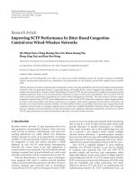
Figure 1: Bayesian network representation of the new model for
gene expression.
where A is an n × n state transition matrix. B is an n × p
input matrix which captures the impacts of the expression
of p regulators on the system. C is a q
× n output matrix
that represents the influence of internal state variables on the
output gene expression level at each time point. z
t
is an n-
dimensional vector collecting the values of n state variables
at time point t. x
t
is a q-dimensional vector collecting
expression values of q genes at time point t. u
t−τ

is a p-
dimensional vector collecting the values of p input variables
at delayed time point t
− τ. w
t
and v
t
are independent
white noises. Compared to the Rangel model, our model
removes the feed-forward matrix, D, assuming that gene-
gene regulation can be captured by indirect regulations
through internal variables instead of direct gene regulation
from one time point to the next. As with the model by
Rangel et al. [10], the product C
× B produces a q × p
matrix that depicts the regulatory relationships between p
regulators and q target genes. The possible values for the time
delay for each of the p regulators, τ
i
,wherei = 1, , p,
is estimated by scanning a range of positive integers, with
the minimum time delay of zero, that is, gene coregulation.
The best fit is determined by minimizing the Akaike’s
Information Criterion (AIC) for the residual variance. AIC
was developed by Akaike [17] to determine a compromise
between the complexity of an estimated model and the fitness
of the model with the data in order to avoid the overfitting
problem. A Bayesian network representation of the model
is shown in Figure 1. From the results in [12, 18], such a
modeling approach can assure that the inferred networks are

stable and controllable.
ThemodelwasimplementedasaMATLABprogram.
tdGRNusesvariousfunctionsfromMATLAB’sControl
System and System Identification toolboxes. The n4sid() and
aic() functions are used for system identification, system
stability, and delay analysis. The n4sid() function imple-
ments the Numerical Algorithms for State Space Subspace
System Identification (NS4SID) proposed by Van Overschee
and De Moor [19]. It computes the parameterization of the
model, solving for the matrices A, B,andC.Thesubspace
algorithm is noniterative and does not depend on a priori
parameterization. This al lows the method to always find a
convergent system and avoids problems such as local minima
and initial condition bias. The system identification is based
on QR and singular value decomposition which ensures that
the estimated linear time-invariant model is stable [19]. The
only requirement for the identification is the order of the
system. In tdGRN, the order is determined by selecting the
model that produces the best AIC score [12]ascomputed
by the aic() function. The lower the AIC score the better the
goodness-of-fit of the estimated state-space model. Finally,
the compare() function is used to determine the overall
model fitness to the data. The model fitness is represented
as a percentage estimated as follows:
fitness
=
⎛
⎝
1 −
norm

(
Yh− Y
)
norm

Y − Y

⎞
⎠
×
100%, (2)
where Y
= (y
0
, y
1
, , y
m
) is the actual gene expression
profile,
Y is the mean of Y ,andYh = (yh
0
, yh
1
, , yh
m
)
is the predicted expression profile from the model. m
is the total number of time points. norm(Yh
− Y)and

norm(Y
− Y ) are the Euclidean distances between the
predicted and the actual expression profiles, and between
the actual expression profiles and mean expression profile,
respectively. Ideally, if the distance between the predicted and
the actual expression profiles is zero, the function returns a
100% fitness. tdGRN supports two types of models: single
input and multiple input models, both with time delays. A
single-input model captures simple one-to-one regulatory
relationships. A multiple-input model works for complex
many-to-one regulatory relations.
2.2. Single-Input Model with D elay. In a simple one-to-one
regulatory relation, the regulation of a gene is highly related
to its transcription factor (TF). In other words, residual
regulation by other factors can be treated as hidden variables,
that is, missing data. Therefore, a single-input and single-
output (SISO) model (TF versus gene or TF versus TF) can
be used to describe the input and output signals. The SISO
model can be applied to identify network motifs such as feed-
forward loops, Multi-component loops, and single-input
motifs as described by Lee et al. [20]. Figure 2 illustrates
how tdGRN is used to model two such network motifs. The
network motifs are shown on the left and the corresponding
state-space models on the right.
According to Lee et al. [20], two anaerobic condition-
related transcription factors in yeast, Rox1 and Yap6, form
a regulatory circuit in which the y regulate each other. The
regulation circuit is represented as a multi-component loop
motif as shown in Figure 2(a), where the over- or under-
expression of one TF regulates the gene expression of another

(i.e., p
= q = 2). In the state-space representation of tdGRN,
the mRNA expression of ROX1 and YAP6 (orange boxes)
over time are the observed values. The TF protein expression
levels, Rox1 and Yap6 (purple ellipses), and possibly other
hidden factors (purple ellipse labelled with a question mark,
“?”) are the hidden variables. At time t, the protein expression
levels are affected by gene expression of ROX1 and YAP6 with
τ
1
and τ
2
input time delays, respectively. The hidden variables
in turn dictate the output gene expressions of ROX1 and
4 EURASIP Journal on Bioinformatics and Systems Biology
t
t + 1
τ
2
τ
1
Multicomponent
loop
Rox1
ROX1
YAP6
Yap6
?
ROX1
YAP6

Rox1
Yap6
?
YAP6 ROX1
Hidden states
Yap6
Rox1
(a)
t
t + 1
τ
2
τ
3
τ
1
,
Feed-forward
loop
Transcription factor
activity
Gene expression
Mcm1
SWI4
Swi4
CLB2
Swi4
Mcm1
MCM1
SWI4

?
?
Hidden states
Swi4
Mcm1
SWI4 CLB2
(b)
Figure 2: An example of SISO state-space representation of the gene regulatory network motifs described by Li et al. [14]. (a)
Multicomponent loop, and (b) feed-forward loop. The network motifs are shown on the left and the corresponding state-space models
on the right. Purple ellipses correspond to protein expression, while the orange rectangles signify gene expression. All uppercase names are
used for transcripts, and mixed upper-and lowercase is used for tran scription factor names. A directed dashed line shows the direction of
translation, while a directed solid line represents the direction of transcription regulation.
YAP6 at time t + 1. The multiple time delay relationships can
be expressed as a 2
× 2 matrix as follows:
⎡
⎣
0 τ
1
τ
2
0
⎤
⎦
. (3)
Recall that this q
× p matrix captures the regulatory
relationship between the p
= 2 regulators and the q = 2
target genes.

Another example of a network motif is the regulation of
CLB2, a G2/M-cyclin gene, and transcription factor Swi4 by
Mcm1.ItisillustratedbyLeeetal.[20] as an example of a
feed-forward motif. The MCM1 gene regulates CLB2 as well
as the Swi4 transcription factor, which also regulates CLB2
cyclin. In this network motif, there are two regulators, two
target genes (i.e., p
= q = 2), and three possible input time
delays, each corresponding to a regulatory relation (refer
to Figure 2(b)). The multiple time delay relationships are
expressed as a 2
× 2 matrix as follows:
⎡
⎣
τ
2
τ
3
0 τ
1
⎤
⎦
. (4)
The time delay, τ
i
, is estimated by scanning a range of
possible integers, with the minimum time delay of zero,
that is, gene coregulation. In the case of yeast cell cycle
data, the maximum number of delays should not exceed the
time for a complete cell cycle (G1

→ S → G2 → M), which is
estimated to be about 60 minutes [13]. For Spellman’s time-
course microarray data [21], since each sampling interval
is 7 minutes, the maximum delay should never exceed 8
sampling intervals (i.e., 60 minutes
× 1sample/7minutes).
Similar to Li et al. [14] but unlike Ota et al. [6] and Sung
et al. [13], we believe that the actual time delay between
binding and transcription is on the order of minutes. This is
based on an assumption that gene transcriptional regulations
are most likely to occur within the same phase or at
the transition point from one phase to another. Since the
longest cell-cycle phase, G1, takes about 25 minutes, the
maximal reasonable delay is less than 3 sampling intervals
(i.e., 25 minutes
× 1 sample/7 minutes). Hence, the default
maximal delay for yeast cell cycle is set at 2 sampling
intervals, that is, 14 minutes, for Spellman’s data [21]. Note
that this default value may not be applicable to other
biological systems.
2.3. Multiple-Input Delay Model. A SISO model may not
work wel l when multiple regulators show significant regula-
tion of a target gene. The presence of two or more regulators
increases the model complexity. In addition, some studies
EURASIP Journal on Bioinformatics and Systems Biology 5
have shown that different gene pairs have different time
delays for gene regulation [13]. Therefore, the multiple time
delay issue should also be addressed. We present a multiple-
input model with time delay in which the transcription
profiles of all known regulators, if available, are provided

as inputs to the system. The input delays are estimated
individually for each regulator. The multiple-input single-
output (MISO) model can be used to determine multi-input
and regulator cascade network motifs, as described by Lee
et al. [20].
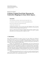
Figure 3 illustrates how tdGRN is used to model a multi-
input network motif. In this example, the gene for the protein
component of the yeast large (60S) ribosomal subunit,
RPL16A, is transcriptionally regulated by three transcription
factors: Fhl1, Rap1, and Yap5 (i.e., p
= 3, q = 1). Assuming
that each TF has zero or some input delay to the regulation
of RPL16A, the multiple time delay relationship can be
described as follows:

τ
1
τ
2
τ
3

. (5)
Recall that this q
× p matrix captures the regulatory
relationship between the p
= 3 regulators and the q = 1
target gene.
The maximum number of input channels allowed in the
model depends on the complexity of the motif structure

and the time delay of each input channel. A greater number
of available time points are required to model a more
complicated network structure. Also, given a grossly limited
number of time points, each additional unit of time delay
reduces the number of available points to train a model and
therefore reduces the reliability of the model. Consider an
extreme case w here a factor F regulates a gene G with 9 units
of time delay. If there are only 10 time points, the regulatory
relationship cannot be modeled since the data will show little
or no evidence of regulation. In the case of Spellman’s yeast
microarray data (18 time points), tdGRN can compute a
stable system for a maximum of four input and four input
delays. In general, the maximum number of input channels
is determined by trial and error and varies depending on the
complexity of the network.
2.4. Network Connectivity. Rangel et al. [10] construct reli-
able gene regulatory networks based on bootstrap statistical
analysis. The method is applied to highly replicated data.
Their approach has a severe limitation, however, b ecause
most currently available time-course microarray data are
either replicated few times (e.g., less than 5) or not replicated
at all. Li et al. [14] use genome-wide location analysis
results to construct a network structure and then infer the
transcription factor activities with mathematical modeling.
The latter approach significantly reduces the number of false
positive node connections since the network connectivity
is predetermined. In addition, the method can be used to
model gene regulatory networks from nonreplicated data.
The limitation of Li’s approach is that it removes the power
Transcription factor

activity
Gene expression
RPL16A
Fhl1
Rap1 Yap5
FHL1 RAP1 YAP5
RPL16A
Rap1
Fhl1
Yap5
Fhl1
Yap5
??
Hidden states
Rap1
t
t + 1
τ
2
τ
1
τ
3
Figure 3: An example of MISO state-space representation of a
multi-input gene regulatory network motif described by Li et al.
[14]. The network motif is shown on the left and the corresponding
state-space model on the right. Purple ellipses correspond to protein
expression, while the orange rectangles signify gene expression. All
uppercase names are used for transcripts, and mixed upper-and
lowercase is used for t ranscription factor names. A directed dashed

line shows the direction of translation, while a directed solid line
represents the direction of tr anscription regulation.
to uncover new connections that are not identified by ChIP-
on-chip data.
In this paper, we present a three-step solution (tdGRN)
such that network connectivity is based on, but not limited
by, genome-wide location analysis results. First, the data
is partitioned into two groups: transcription factors (TFs)
and target genes (TGs). Each TF is a possible regulator of
another TF and/or TG. Secondly, using the n4sid() function,
tdGRN creates an initial set of network connections based
on the location analysis results. All the TF versus TF and
TF versus TG regulatory relations derived at this stage are
screened for potential corresponding state-space models.
Only the potential regulator y relations which satisfy the
goodness-of-fit criter ia are recorded and subjected to the
next round of analysis. For each TF, tdGRN records the
optimized parameters: initial state, number of time delays,
the number of states (variables) that reflects the complexity
of the regulations. In the third step, tdGRN per forms an
additional round of network connection screening based
on the regulation parameters generated in the second step.
For example, if a transcription factor F regulates n TGs
with time delay τ, the tdGRN program will attempt to
recruit other genes that have not been identified as targets
of F but possess regulatory relations with F that resemble
the existing ones. This is based on a common assumption
that genes with high correlation in expression profiles are
likely to be coregulated [1, 2, 22, 23]. The additional round
of network screening is implemented by MatLab’s pem()

function which is an alternative to the N4SID algorithm that
uses a prediction error model (PEM) for parameterization.
According to Favoreel et al. [24], the latter algorithm is
relatively more sensitive compared to N4SID once the initial
parameters are determined.
In addition, tdGRN generates a network output file that
can be directly imported into Cytoscape [16] for network
visualization, integration, and analysis.
6 EURASIP Journal on Bioinformatics and Systems Biology
Table 1: Parameters for the artificial data. The artificial data involves 2 regulators (R1, R2) and 9 genes (G1–G9).
Names Function Delay (τ)Regulatedby
Regulator R1 sin(x)N/AN/A
Regulator R2 cos(x)N/AN/A
Gene G1 sin(x)+v 0R1
Gene G2 sin(x + τ)+v 1R1
Gene G3 sin(x +2τ)+v 2R1
Gene G4 cos(x)+v 0R2
Gene G5 cos(x + τ)+v 1R2
Gene G6 cos(x +2τ)+v 2R2
Gene G7 sin(x)+cos(x)+v 0 R1+R2
Gene G8 sin(x + τ)+cos(x + τ)+v 1 R1+R2
Gene G9 sin(x +2τ)+cos(x +2τ)+v 2 R1+R2
3. Results
3.1. Data Sets. Two data sets are used in this study. First,
an artificial data set is created to validate the model. There
are several methods proposed in the literature to create
appropriate artificial gene expression data [25, 26]. The
artificial data is created in this study by a method similar to
that of Yeung et al. [26]; that is, (1) mimicking the periodic
property of cell-cycle microarray data, (2) simulating the

systematic errors in microarray experiments, (3) containing
multiple time delay relations between regulators and targets.
Secondly, we apply our model to analyze the yeast cell cycle
microarray data published by Spellman et al. [21]. Details of
both data sets are described in the following sections.
3.1.1. Artificial Data. The artificial data consists of data
streams of 2 regulators, R1 and R2, and 9 target genes, G1,
G2, , G9. To simulate cell cycle gene expression data, the
artificial data is created by using sine and cosine functions
listed in Table 1. G1 to G3 are associated with R1 with delays
τ
= 0, 1, 2, respectively. G4 to G6 are associated with R2
with delays τ
= 0, 1, 2, respectively. These relatively simple
cases test the ability of the model to associate the target genes
to their regulators, and to predict the number of the delays.
G7 to G9 are associated with both R1 and R2 with delays τ
= 0, 1, 2, respectively. In these more complex cases, we test
the ability of the model to connect the target genes to the
multiple regulators, and to predict the number of the delays.
Each data stream has a uniformly distributed random noise,
v, in the range of
−0.05 to 0.05 (i.e., one twentieth of the
range of sine and cosine functions), assigned to each time
point.
3.1.2. Yeast Cell-Cycle Data. The second data set used in
this study consists of 800 expression profiles of alpha
factor-based yeast cell-cycle genes studied by Spellman
et al. [21]. The microarray hybridizations were done using
asynchronous yeast cells sampled every 7 minutes for 18

time points. Normalized expression data were downloaded
from the Stanford Microarray Database (SMD) [27]. No
further pre-processing was done. The knnimpute() function
from MATLAB’s Bioinformatics toolbox was used to impute
missing data.
In this study, it is assume that (1) the experimental
time points capture biologically significant changes, but
(2) there exist effects of hidden variables in the biological
system that cannot be measured in a gene expression
profiling experiment, for example, missing data for mRNA
degradation.
In the following, we first describe the output of modeling
the artificial data and the lessons learned in the modeling
process. Then we present the results of modeling the yeast
cell-cycle expression data. The global regulatory network
diagram is presented as well as detailed analysis of G1- and
B-type cyclins. Finally, we illustrate the capability of tdGRN
in selecting the most feasible regulatory mechanism from
multiple models.
3.2. Modeling a Gene Network Using the Artificial Data. To
demonstrate the difference between the SISO and MISO
models, we first apply only SISO to network prediction
on the artificial data. The two regulators, R1 and R2, are
expected to connect to the target genes, G1 to G9, as
described in Tabl e 1. Figure 4 is a graphical representation
of the produced SISO network. The network visualization
is generated using Cytoscape where each node represents a
gene and each directed edge represents a predicted regulatory
relationship between a regulator and the target gene. Each
edge is labelled with the predicted number of input time

delays. Eleven out of twelve edges are identified by tdGRN-
SISO. Among the eleven, 9 edges are annotated with the
correct time delays. The complete output of tdGRN-SISO
is tabulated in Tabl e 2. The “Order” column gives the order
of the system that reflects the model complexity. “Fitness
(%)” (percentage of fitness) reflects the goodness-of-fit of the
state-space model to the data. The “AIC” column contains
the Akaike’s Information Criterion score. The best-fitted
model is selected by minimizing the AIC score.
EURASIP Journal on Bioinformatics and Systems Biology 7
G1
G2
G3
G4
G5
G6
G7
G8
G9
R1
R2
0
0
0
00
111
222
Figure 4: SISO output for artificial data. All edges are labeled
with the predicted time delays. A blue edge represents a correct
interaction; a red edge represents an incorrect one.

G7 G8 G9
R2R1
0
0
1
1
2
2
Figure 5: MISO output for artificial data.
Table 2: SISO output for the artificial data.
Regulator Target Order Delay (τ) Fitness (%) AIC
R1 G1 1 0 98.76 −9.0735
R1 G2 1 1 98.76
−9.1076
R1 G3 1 2 98.68
−8.9094
R1 G8 2 0 82.40
−3.9379
R1 G9 1 0 81.44
−3.2183
R2 G4 1 0 98.70
−8.8321
R2 G5 1 1 98.66
−8.9243
R2 G6 1 2 98.82
−9.1675
R2 G7 2 0 85.69
−5.0339
R2 G8 2 1 82.82
−4.3840

R2 G9 2 2 83.31
−4.2520
Table 3: MISO output for artificial data.
Regulator Target Order Delay (t1,t2) Fitness (%) AIC
R1,R2 G7 1 0,0 99.27 −8.0843
R1,R2 G8 1 1,1 99.18
−8.6052
R1,R2 G9 1 2,2 99.15
−8.4814
The results show that the SISO model can predict 100%
correctly the one-to-one regulations but not the many-
to-one regulations. For many-to-one regulations, the SISO
modeldetects5outof6(
∼83%) of them, but only 3 out
of 6 are predicted with correct delays. As expected, almost
all predicted connections (4 out of 5) from the many-to-
one regulation are in higher-order state-space systems (i.e.,
second-order state-space systems) compared to the rest.
tdGRN-SISO predicts a more complex regulation mecha-
nism in these systems and produces poorer scores for the
percent of fitness and AIC. The fact that the SISO model can
identify most of the regulatory relations in our simulation
suggests that, in the absence of a priori knowledge of the
network structure, the single-input single-output model may
be used to detect more complex network connections but the
number of time delays and the order of the system may need
to be reassessed using a MISO model.
We applied the tdGRN-MISO model for network predic-
tion of the G7 to G9 genes. Given the knowledge that R1 and
R2 co-regulate G7, G8, and G9, tdGRN-MISO can correctly

predict 6 out of 6 edges and the corresponding number
of time delays. Figure 5 is a graphical representation of the
results. The complete output of tdGRN-MISO is shown in
Table 3. Note that the tdGRN-MISO can produce much
better models (better than 99% fitness, and much lower
AIC scores) than tdGRN-SISO for these cases. The results
illustrate the advantage of incorporating potential regulatory
relationships into the modeling process.
3.3. Modeling the Gene Networks in Saccharomyces cere visiae
3.3.1. Learning the Network Structure. The genome-wide
location analysis results of nine known cell-cycle related
transcription factors (Swi4, Swi6, Mbp1, Mcm1, Ace2, Swi5,
Fkh1, Fkh2, and Ndd1) were from the study of Young’s
lab [28]. The results are reported as P-values that reflect
the significance of the binding between TFs and the corre-
sponding promoter regions. We considered a P-value less
than or equal to 0.01 as being significant. This cutoff is less
stringent than the 0.001 cutoff proposed by Lee et al. [20]. A
relaxed threshold was selected to reduce the number of false
negatives in location analysis. Complementarily, the number
of false positives is controlled by providing cross-validation
evidence from the modeling of time-series gene expression
data. Based on the location analysis results and the selected
cutoff, we identified 301 out of 800 cell-cycle regulated genes
reported by Spellman et al. [21] which bound to at least
one of the nine TFs. Refer to Table 1 in the supplementary
material available on line at doi: 10.1155/2009/484601. for
the list of the 301 genes and the binding map to the nine TFs.
In that table, a “+” character in a cell represents a significant
binding (P

≤ 0.01).
3.3.2. Modeling the Gene Network. We applied tdGRN to the
301 cell-cycle regulated genes identified above. It predicted
the regulation models of 93 genes or approximately 31% of
the total input genes. The results are tabulated and shown
in Supplementary Table 2. On a Pentium III 800 MHz
computer, the total run time for tdGRN to analyze the 301
genes was approximately 90 minutes.
Almost half of the 93 genes are regulated in the G1
phase and about 25% are regulated in the G2/M phase.
Compared to the 301 input genes, this represents a minor
increase in percentage of genes regulated in G1 phase (36%
to 44%), and a slight decrease for M/G1 phase (17% to
12%). The differential success rates in modeling G1- and
8 EURASIP Journal on Bioinformatics and Systems Biology
HHF1
FKH1
CLN1
CIN4
YPL267W
MNN1
MSH6
ASF1
SVS1
AD2
PRY2
YNR009W
ERP3
YDR528W
YIL141W

YHR149C
SPK1
SRO4
HTB2
SPT21
YGR248W
YGR151C
SIM1
RFA1
YOX1
HTA1
RSR1
HHO1
CLB6
CLB5
CLN2
BBP1
RFA2
SMC3
HTB1
HTA2
YNL300W
YGR189C
YGR086C
YIL177C
YHB1
SWI5
YGR296W
CTS1
HSP150

SCW11
EGT2
ACE2
SIC1
AGA1
CLN3
BUD9
AGA2
MCM1
GPA1
UTR2
TSL1
PIC1
YMR031C
CDC21
SWI4
SWI6
MBP1
YLR190W
MFA2
RNR1
PHO11
CLB2
YDR451C
YMR215W
KIN3
YDR033W
FIR1
IQG1
NDD1

CDC5
SPO12
ALK1
PRY1
BUD4
CIS3
YIL58W
SML1
HST3
YNL058C
YPL141C
YJL051W
YCL063W
CDC20
FKH2
PDS1
CDC46
AT R1
SVL3
KIP2
CIK1
YMR144W
YOL030W
FTR1
MCD1
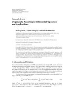
Figure 6: Gene regulatory network of 93 cell-cycle regulated genes. For greater clarity, genes are represented by white nodes and transcription
factors are represented by yellow nodes. All node labels are shown using capital letters, irrespective of whether the node represents a
transcription factor or a regulated gene. There is no significance to the size of circle used to represent nodes.
M/G1-regulated genes may be due to the differences in
the number of TFs from each phase. There was no M/G1-

specific transcription factor used in this study. On the other
hand, there were three (Swi4, Swi6, Mbp1) G1-activated
TFs.
Among the nine transcription factors, Swi4, Swi6, and
Mbp1 are known to play important roles in G1 and late G1
phasegeneregulation[28, 29]. The three TFs constitute two
transcription factor complexes: SBF (Swi4 and Swi6), and
MBF (Swi6 and Mbp1). SBF and MBF control over 50% of
the total detected regulatory relations in our model. Figure 6
depicts the modelled network. In this network diagram,
each yellow node represents a TF and each white node
represents a target gene. A directed arrow between a TF and
a target gene node represents a detected regulatory relation.
Figure 6 reveals a large cluster of target genes regulated by
combinations of SBF and MBF (left side of Figure 6). The
fork-head transcription factors Fkh1 and Fkh2, and Ndd1
regulate a smaller cluster of G2/M-phase expressed genes
on the right of the network diagram. Among the modelled
genes in the two most abundant phases, the regulation
of G1 phase’s G1-cyclins (CLN1, CLN2, and CLN3) and
G2/M phase’s B-type cyclins (CLB2, CLB5, and CLB6)
are identified. T he modelled regulatory mechanisms of the
cyclins were further investigated. The results are discussed in
the following subsection.
3.3.3. Regulation of G1- and B-Type Cyclins. We examined
more closely the regulation models of 3 G1-cyclins (CLN1,
CLN2, and CLN3) and 5 B-type G2/M-cyclins (CLB1, CLB2,
CLB4, CLB5, and CLB6). These two sets comprise all the
CLN and CLB cyclins in the data set (CLB3 was not
present). The CLN and CLB cyclins were selected due to

their important roles in cell-cycle regulation and relatively
EURASIP Journal on Bioinformatics and Systems Biology 9
Table 4: tdGRN output for yeast cyclins regulatory network.
Regulator Target Order Delay (τ) Fitness (%) AIC Binding evidence
Fkh1 CLB2 2 0 73.465076 −2.510095 Y
Fkh1 SWI4 2 0 71.941152
−3.016292 N
Fkh2 CLB2 2 0 69.618154
−2.677518 Y
Fkh2 SWI4 2 0 71.553277
−2.617587 N
Fkh2 CLB1 2 0 71.09556
−2.485664 N
Mbp1 SWI4 2 2 62.060827
−1.539307 Y
Mbp1 CLB2 2 2 64.177229
−2.604613 Y
Mbp1 CLN2 2 1 61.249674
−0.918211 Y
Mbp1 CLB1 2 2 60.996793
−2.303097 N
Mcm1 SWI4 2 1 67.744846
−2.430281 Y
Mcm1 CLB2 2 2 64.483538
−2.042422 Y
Ndd1 CLB2 2 2 73.178501
−1.628935 Y
Ndd1 CLN1 2 2 60.400341
−1.758735 Y
Ndd1 CLB6 2 0 71.960519

−1.687905 Y
Ndd1 CLB5 2 0 65.499866
−2.475658 Y
Ndd1 FKH2 2 2 72.445931
−3.800203 N
Ndd1 CLN3 2 2 65.957132
−2.655417 N
Swi4 CLB2 2 2 68.538231
−1.872905 Y
Swi4 CLN3 2 1 60.289651
−3.029056 Y
Swi4 CLN2 1 0 64.906209
−1.360941 Y
Swi4 CLN1 1 0 65.22902
−2.237727 Y
Swi4 CLB6 2 0 73.243562
−2.039319 Y
Swi4 CLB5 2 0 75.557682
−2.937196 Y
Swi4 FKH2 2 1 68.484476
−3.41278 N
Swi4 CLB1 2 2 77.002957
−2.119164 N
Swi6 SWI4 2 0 70.893228
−1.993188 Y
Swi6 CLB2 2 2 63.223062
−1.786548 Y
Swi6 CLN2 2 2 61.366645
−0.473000 Y
Swi6 CLN1 2 2 61.383819

−1.329583 Y
Swi6 ACE2 2 0 62.457434
−1.956277 N
well-studied regulatory mechanisms. Figure 7 is a diagram
produced by tdGRN which features the selected genes.
Each node represents a gene or a transcription factor, each
directed edge represents a regulatory relation, and each
edge label denotes the regulatory delay between two nodes.
For example, Swi6
→ CLN2 has a delay of 2 samples (i.e.,
2
× 7 minutes/sample = 14 minutes). The network edges
are color coded such that a red edge represents a known
interaction based on location analysis and a blue edge
represents an unknown relationship.
The tdGRN technique uncovered a network of 15 nodes
with 30 edges. 21 out of the 30 edges (i.e., 70%) have known
regulatory relationships. The average model fitness is 67%.
A tabulated output is provided in Table 4, in which the
column “Order” means the order of the system which reflects
the model complexity. The percentage of fitness reflects the
goodness-of-fit of the state-space model to the data. AIC is
the Akaike’s Information Criterion score. Among the novel
regulatory relations determined, there is evidence to support
Swi6
→ CLN2 [29], Fkh2 → CLB1 [30], Ndd1 → FKH2 [31]
regulation proposed in the literature.
3.3.4. Regulation of CLN2. The tdGRN technique uncovered
the regulatory relationship between Swi6 and CLN2 (with
order

= 2 and delay = 2) that is not reported in the location
analysis results (see Supplementary Table 1). As mentioned
in the previous section, Swi4 and Swi6 encode a heterodimer
complex, SBF. It has been shown that SBF induces CLN2
transcr iption in the late G1 phase [28]. In our modeling, we
detected the regulatory relations of Swi4
→ CLN2 with a first-
order system (AIC score
= −1.36), and Swi6 → CLN2 with a
second-order system (AIC score
= −0.47). The difference in
the AIC score indicates that although both TFs contribute
to the regulation of CLN2, Swi4 represents a better model
to control CLN2 regulation than Swi6. This finding is
interesting in view of the observation that Swi4 is the DNA-
binding component of the SBF complex and that interactions
with Swi6 afford binding of Swi4 to DNA [31].
10 EURASIP Journal on Bioinformatics and Systems Biology
Table 5: MISO output for the CLN2 regulation.
Regulators (R1,R2) → Target Order R1 R2 Fitness (%) AIC Best fit
Delay Delay
(Swi4, Swi6) → CLN2
1 0 1 64.798724
−2.566028
∗
1 0 2 66.922105 −2.889358
2 0 0 67.240317
−0.892564
2 0 1 65.115198
−0.894492

FKH1
FKH2
CLB2
CLB1
CLB6
CLB5
CLN1
CLN2
CLN3
MBP1
MCM1
2
2
2
2
2
2
2
2
2
2
2
2
2
0
0
0
0
0
0

0
0
0
0
0
SWI4
SWI6
NDD1
ACE2
1
Figure 7: Gene regulatory network for the G1- and G2/M-cyclins.
A red edge represents a known interaction based on location
analysis and literature search; a blue edge represents an unknown
relationship.
Using the SISO model, we demonstrated that Swi4 and
Swi6 regulate CLN2 with input delays of 0 and 2, respectively.
The fitness of the corresponding models is 65% and 61%,
respectively. We applied tdGRN-MISO to this data in an
attempt to improve the model of CLN2 gene expression.
tdGRN-MISO produces 4 possible models (see Ta ble 5 ).
The best-fitted model based on AIC score (noted with
an asterisk) is a first-order system with fitness equal to
67%, delays τ
Swi4
= 0andτ
Swi6
= 2. Compared to the
previously mentioned 2 SISO models, the MISO model is
relatively better in terms of both AIC score and the overall
percent fitness. These results suggest that Swi4 and Swi6 do

regulate CLN2 transcription in a combined manner. This is
in agreement with biological fact that Swi6 is the modifying
factor whose translocation to the nucleus and binding to
SWI4 are required for Swi4 to bind to DNA [32].
3.3.5. Regulation of CLB2. CLB2 encodes a B-type cyclin that
activates the cyclin-dependent kinase, CDC28, to promote
the transition from G2 to M phase of the cell cycle. The
Fkh1
Swi4
CLB2
2
0
0
(a)
Ndd1 Fkh2
CLB2
2
2
0
(b)
Mbp1 Swi4
CLB2
2
2
2
(c)
Swi4
CLB2
Mcm1
2

2
1
(d)
Figure 8: Feed-forward loop network motifs in the regulation of
CLB2 found by tdGRN. Each edge is labeled with the value of time
delay. A red edge represents a known interaction based on location
analysis and literature search; a blue edge represents an unknown
relationship.
promoter region of the CLB2 gene contains cis-element
binding sites to 10 different transcription factors [33]
according to Harbison et al. [34]. The binding motifs are also
confirmed by the ChIP-on-chip results (see Supplementary
Table 1). Using the cutoff of P
≤ 0.01, seven out of nine TFs
(i.e., Fkh1, Fkh2, Ndd1, Mcm1, Mbp1, Swi4, and Swi6) show
significant in vivo binding to CLB2.
The transcription factors that are found at the CLB2
promoter regions are known to regulate genes at different
cell-cycle phases. For example, the SBF (Swi4, Swi6) and
MBF (Swi6, Mbp1) complexes promote G1 to S phase
transition, Mcm1 regulates late G2 and some M/G1 genes,
and Ndd1 functions at the G2/M phase [30]. Hence, it
is unlikely that all binding factors are functional and are
active at the same time. Using the tdGRN, we detected
regulatory relationships of the seven TFs to CLB2 (see
Table 4). Furthermore, a closer look at the regulation of
CLB2 reveals four feed-forward loop (FFL) network motifs
(see Figure 8). A network motif is a biochemical wiring
pattern that recurs throughout transcriptional networks.
The feed-forward loop (FFL) is one of the most common

EURASIP Journal on Bioinformatics and Systems Biology 11
network motifs found in the bacterium Escherichia coli and
the yeast Saccharomyces cerevisiae [35]. A feed-forward loop
is a three-gene motif incorporating two input transcription
factors: a master and a secondary regulator. The master
regulator regulates the secondary regulator and they both
jointly regulate a target gene. We present the four FFLs
found by the tdGRN-SISO in Figure 8. The top-left node is
the master node of the FFLs. They are Fkh1, Ndd1, Mbp1,
and Mcm1. The top-right node is the secondary regulator
and this is Swi4 except when the master node is Ndd1 in
which case the secondary regulator is Fkh2. The average SISO
model fitness for each TF
→ CLB2 regulation is 68%. All
TFs except the fork-head TFs, Fkh1 and Fkh2, have delay of
2 sampling intervals. Among the four FFLs, the regulatory
relationship Mcm1+Swi4
→ CLB2 is also reported by Simon
et al. [28] as an FFL using only the location analysis data with
P
≤ 0.001.
Mangan and Alon [35] suggest that one important
function of FFLs is to speed up the response time of
the transcription networks. That is, although positive gene
regulation can be efficiently achieved by increasing the
concentration of the TF gene’s protein product, the response
time is governed by the lifetime of the protein product, which
is often much longer. Therefore, one way to speed up the
response is to increase the degradation rate of the protein
product through a second regulator and perhaps to block

access to the target gene’s binding site by the first TF protein
product. Since the later regulator controls the expression of
the former TF (the secondary regulator) and the target gene,
it is called the master regulator. At the transcr ipt level, one
would expect the target gene expression level to be a function
of the expression of both regulators as the FFL mechanism
should be functional.
We applied tdGRN-MISO to the four FFL motifs identi-
fied by the SISO model for CLB2 regulation. We hypothesize
that if an FFL is present, one would expect the master and
secondary regulators to work in a collaborative manner.
That is, the unexplained variation seen in the principal TF’s
regulation can be elucidated by the feed-forward regulation
of the secondary TF, and vice versa. On the other hand, if
the FFL is inactive or if only one of the two regulators works,
then the model wil l not be improved by tdRGN-MISO and
the percent fitness of the model will remain roughly the same
or be worse.
The output of tdRGN-MISO is tabulated in Tabl e 6.The
best-fitting model is marked with an asterisk in the rightmost
column. The best model for Fkh1+ Swi4
→ CLB2 at ∼80%
fitness is a first-order system with zero time delay for Fkh1
and 2 time delays for Swi4. The best model for Mbp1+Swi4
→
CLB2 is a second-order system with zero time delay for Mbp1
and Mbp2 time delays for Swi4. The fitness is
∼82%. We
did not observe significant improvements in terms of percent
fitness for the Ndd1 + Fkh2 and Mcm1 + Swi4 models. This

suggests that only the former two out of the four possible
FFLs are likely to control CLB2 regulation, and indicates
improvements in model fitness for the Mbp1 + Swi4 and
Fkh1 + Swi4 models over the Ndd1 + Fkh2 and Mcm1 + Swi4
models, which supports our hypothesis.
4. Discussion
Transcription is a very complex process that entails assembly
of multiprotein complexes and enzymatic reactions, and the
ultimate transcript output also depends on temporal factors
that are not amenable to accurate a nalysis. In gene-gene
interactions and in multigenic interactions (networks), the
temporalaspectshaveappreciablebiologicalconsequences
but these causal factors not readily deciphered. Delineating
all these in terms of reverse engineering a genetic system
requirescollectionsoflargeandreplicateddatapoints
that are commensurate with the complexity of the system
and its components and also requires the computational
power to analyze the data. Both can present difficulties,
considering the inherent complexity. Against this backdrop
is the adaptation of models that have originally been used
in reverse engineering physical systems. State-space model is
one such method. It has the advantage of taking the dynamic
changes of gene expression into consideration unlike static
models such as hierarchical or k-means clustering. The data
points (gene expression levels) are treated as observation
variables that arise from linear combinations of the internal
variables in the living system that are intractable due to
technicality or impra cticality. This method is adaptable to
data collection that is missing some points and also to data
that are not highly replicated.

Transcriptomics studies have generated the most exten-
sive datasets in genomics. Microarray analysis is being used
increasingly to determine the expression patterns of tens
of thousands of genes simultaneously. When the expression
pattern of the same genes under two or more intracellular
conditions (e.g., due to innate physiological changes or due
to changes in the growth temperature) is determined, there
is a potential opportunity to discern gene-gene connectivity
with respect to the changing internal environment. However,
microarray data only measures the steady-state levels of the
RNA product, and all other factors such as the level of DNA-
binding factors (e.g., transcription factors; TF) are hidden
variables. A pertinent question here is, “what is the impact of
the delay in making the product of Gene 1 on Gene 2 if Gene
1 is impacting the transcription of Gene 2?” In this regard,
the model developed in this study is useful.
4.1. Discrete versus Quantitative Models. Yeast cell-cycle reg-
ulated genes demonstrate a periodic pattern [20]. The gene
expressions are known to be phase specific. The expression
data are reported as log
2
(sample expression/reference expres-
sion). That is, one measures the changes in expression with
respect to a common reference instead of absolute expres-
sion. A 2-fold change in expression, that is,
|log
2
(ratio)|≥1,
is generally considered significant. It is important to note that
anegativelog

2
(ratio) does not imply inactivity of a regulator.
Instead, it means that the gene expression level is relatively
lower (by the fold change) compared to the control sample,
for example, the time zero sample.
Among the five state-space or Bayesian network solutions
referred to in this work, the models published by Sung et al.
[13]andLietal.[14] use discrete (binary or Boolean)
12 EURASIP Journal on Bioinformatics and Systems Biology
Table 6: Multiple-input and single-output regulatory relations for CLB2.
Regulators (R1,R2) → Target Order R1 R2 Fitness (%) AIC Best fit
Delay Delay
(Fkh1,Swi4) → CLB2
1 0 1 63.644575
−1.537761
∗
1 0 2 79.773793 −3.229595
1 1 0 61.814689
−1.510308
1 1 2 70.844626
−1.853543
2 0 0 71.974595
−1.759781
2 0 1 76.75773
−2.140303
2 0 2 75.445502
−2.533515
2 1 0 74.935231
−3.046253
2 1 1 74.816372

−1.912746
(Ndd1,Fkh2) → CLB2
1 0 1 61.692141
−0.711095
∗
1 0 2 69.823501 −2.268478
1 1 0 60.652689
−0.637223
1 1 2 74.517609
−1.745955
1 2 0 72.64509
−1.793645
1 2 1 69.148994
−1.644347
2 0 0 74.392399
−0.98651
2 0 1 75.908715
−1.714605
2 0 2 78.764701
−1.941071
2 1 0 71.297965
−0.877083
2 1 1 74.106334
−1.081118
2 1 2 69.865951
−2.514543
2 2 0 70.654615
−1.453532
2 2 1 70.375696
−2.480809

(Mbp1,Swi4) → CLB2
1 1 0 65.281567
−1.531062
∗
2 0 2 82.284591 −2.228897
(Mcm1,Swi4) → CLB2
2 0 0 76.835382 -1.577900
∗
2 0 1 78.146638 −1.707728
2 1 1 76.606035
−1.755346
2 1 2 60.319422
−1.722575
2 2 0 63.90925
−1.804213
2 2 1 65.281011
−1.704606
2 2 2 60.778085
−2.139843
profiles of gene expression. However, discrete models suffer
from an inherent difficulty. Finding a reasonable threshold
to define the inactive and active states of gene expression is a
nontrivial task. The basal level of expression varies by several
orders of magnitude among some genes. In such cases, the
fold-change values alone cannot define the on-off state. For
a gene whose state is defined as “off ” in a discrete model
because of a fold-decrease value at time
= 1 might, in fact,
still be substantially a ctive if its basal level was high (at time
= 0). Consequently, the on-off states of various genes in

a microarray are not definable on the basis of comparing
their fold-changes alone. Soinov et al. [36] have proposed
an alternative method to bypass the assumption of arbitr ary
discretization thresholds for the regulators. Their states of a
“predicted gene” (i.e., a target gene) are determined by the
quantitative expression levels (or changes in the expression
with respect to a control sample) of the “explaining genes”
(i.e., the regulators). The results are presented in the form
of a rooted decision tree such that the states ( up-/down-
regulated, or expressed/not expressed) of a target gene (leaf
node) are determined by the combinatorial decision rules of
the regulators (nonleaf nodes). The Soinov et al. approach
[36] can potentially improve the performance of discrete
network models.
On the other hand, the biggest challenge in quantitative
modeling is the inherent noise in the expression data.
Especially when a gene is expressed at a low level, a low
signal-to-noise ratio causes an inaccurate measurement of
fold-change. This will in turn affect the ability of quantitative
models in learning the network str ucture and in getting good
model fitness. In this study, the average model fitness for
yeast expression data is 67%.
EURASIP Journal on Bioinformatics and Systems Biology 13
4.2. Gene Regulatory Network: What, When, and How. A
ChIP-on-chip experiment, in the context of our work,
answers the question: what are the potential targets of a
given TF? The evidence of in vivo protein-DNA interactions
can help biologists to uncover regulatory network structure
[14, 20, 28]. However, the binding of a protein to a gene
sequence does not necessarily indicate a regulatory outcome.

In yeast, a B-type cyclin, CLB2, is known to have cis-
element binding sites for 10 different transcription factors
[34]. Many of these transcription factors are known to
regulate genes at different cell-cycle phases. It is unlikely
that all binding factors are functional at the same time.
Our modeling tool provides a w ay to model gene regulation
based on time-course expression data. In this document,
we analyzed 301 cell-cycle regulated genes with possible
regulatory relationships to at least one of the nine known
transcr iption factors. Among these, we are able to identify
and model the regulation mechanisms of 93 (
∼31%) genes.
Analysis of the time taken by a gene to reach its full
expression level (peak time) provides insights into when
a gene is maximally expressed during the cell cycle. The
understanding of gene expression timelines is useful for
associating a time factor to the physiological changes in cells.
However, the duration for a gene to reach its peak expression
in a cell-cycle alone is not enough to constitute the full
picture for gene regulation. For example, the transcription
factor complex, SBF (Swi4 + Swi6), regulates CLN1 and
CLN2 transcription in the late G1 phase and drives the
transition into S phase. The peak times for Swi4 and Swi6
are 13% and 37%, respectively. The peak times for the
SBF regulated genes CLN1 and CLN2 are 25% and 23%,
respectively. One component of the SBF regulator, Swi6,
reaches the peak time later than both CLN1 and CLN2. This
shows that the peak time analysis does not convey informa-
tion on how genes are regulated. One may hypothesize that
Swi4 is the rate determining factor in the regulation of the

cyclins and that the G1 cyclins will quickly reach their peak
expressions at 25% after Swi4 reaches its peak at 13%. Our
modeling results support the above mentioned assumption
(refer to Section 3). The Swi4 and Swi6 transcription factors
regulate CLN2 transcription in a combinatorial manner. The
percent fitness of the Swi4 + Swi6
→ CLN2modelisbetter
than t wo separated single-input and single-output models.
Interestingly, our modeling results also suggest that CLN2 is
regulated by both Swi4 and Swi6, and CLN1 is regulated only
by Swi4. This could be the result of relatively weaker role
of Swi6 in cyclin regulation as Partridge et al. have shown
that MCB core elements of both CLN1 and CLN2 depend
primarily on SWI4 [37].
4.3. Model Overfitting. The tdGRN uses location analysis
results to help identify the TF and target gene pairs. This
significantly reduces the risk of overfitting by filtering out the
unrelated inputs (i.e., unwanted noise). In addition, Akaike’s
Information Criterion [17] is applied to the model selection
process. The AIC discourages the selection of a higher-order
system by imposing a penalty for the complexity of the
estimated model. It attempts to find the best goodness-of-fit
with a minimum system complexity. This provides another
guard ag ainst overfitting.
5. Conclusions and Future Work
We have developed a new modeling tool, tdGRN, for
determining prospective gene regulation models from time-
series gene-expression data. The tool has been demonstrated
on artificial data and yeast cell-cycle gene-expression data.
Using the yeast microarray data, we have illustrated that our

model can help identify regulatory relations with multiple
time delays. The model complements ChIP-on-chip results
by predicting the most probable gene regulatory relatioships
between transcription factors and their target genes. The
tool also identifies previously unknown regulatory relation-
ships. For example, in the regulation of G1- and B-type
cyclins, tdGRN uncovers 30 regulation relationships in a
network with 15 nodes, 9 of which are novel findings. The
existing literature contains support of these novel findings
[29–31].
The tdGRN tool uses genome-wide location analysis data
to reveal the primary network structure. Additional regula-
tory relationships can be determined by goodness-of-fit of
alternate models. It should be interesting to compare this
method to the learning-by-modification method developed
by Sung et al. [13] where the network structure is based
on a backward elimination mechanism. Another important
facet of future work would be a systematic study of the
effect of noise on tdGRN. The current version of tdGRN
has a command line user interface. Some features can be
implemented to increase user friendliness. Examples include
a GUI and a facility to load multiple experiments.
Acknowledgment
The authors thank Natural Sciences and Engineering
Research Council of Canada (NSERC) for a partial financial
support to this research.
References
[1] M. B. Eisen, P. T. Spellman, P. O. Brown, and D. Botstein,
“Cluster analysis and display of genome-wide expression
patterns,” Proceedings of the National Academy of Sciences of

the United States of America, vol. 95, pp. 14863–14868, 1998.
[2] M. F. Ramoni, P. Sebastiani, and I. S. Kohane, “Cluster analysis
of gene expression dynamics,” Proceedings of the National
Academy of Sciences of the United States of America, vol. 99, pp.
2266–2278, 2002.
[3] N. Belacel, Q. Wang, and M. Cuperlovic-Culf, “Clustering
methods for microarray gene expression data,” OMICS: A
Journal of Integrative Biology, vol. 10, no. 4, pp. 507–531, 2006.
[4] R. L. Bar-Or, R. Maya, L. A. Segel, U. Alon, A. J. Levine, and M.
Oren, “Generation of oscillations by the p53-mdm2 feedback
loop: a theoretical and experimental study,” Proceedings of the
National Academy of Sciences of the United States of America,
vol. 97, pp. 11250–11255, 2000.
[5] B. Vogelstein, D. Lane, and A. J. Levine, “Surfing the p53
network,” Nature, vol. 408, no. 6810, pp. 307–310, 2000.
14 EURASIP Journal on Bioinformatics and Systems Biology
[6] K. Ota, T. Yamada, Y. Yamanishi, S. Goto, and M. Kanehisa,
“Comprehensive analysis of delay in transcriptional regulation
using expression profiles,” Genome Informatics, vol. 14, pp.
302–303, 2003.
[7] F. X. Wu, W. J. Zhang, and A. J. Kusalik, “Modeling gene
expression from microarray expression data with state-space
equations,” Pacific Symposium on Biocomputing, vol. 9, pp.
581–592, 2004.
[8] X. Hu, M. Ng, F. X. Wu, and B. A. Sokhansanj, “Mining, mod-
eling, and evaluation of subnetworks from large biomolecular
networks and its comparison study,” IEEE Transactions on
Information Technolog y in Biomedicine, vol. 13, no. 2, pp. 184–
194, 2009.
[9] C. Rangel, J. Angus, F. Falciani, et al., “Modelling t-cell

activation using gene expression profiling and state space
models,” Bioinformatics, vol. 20, pp. 1361–1372, 2004.
[10] C. Rangel, J. Angus, Z. Ghahr amani, and D. L. Wild,
“Modeling genetic regulatory networks using gene expression
profiling and state space models,” in Probabilistic Modelling in
Bioinformatics and Medical Informatics, pp. 269–293, Springer,
Berlin, Germany, 2005.
[11] M. Dasika, A. Gupta, and C. D. Maranas, “A mixed integer
linear programming (MILP) framework for inferring time
delay in gene regulatory networks,” Pacific Symposium on
Biocomputing, vol. 9, pp. 474–485, 2004.
[12] F. X. Wu, W. J. Zhang, and A. J. Kusalik, “State-space model
with time delays for gene regulatory networks,” Journal of
Biological Systems, vol. 12, no. 4, pp. 483–500, 2004.
[13] W. Sung, T. Liu, and A. Mittal, “Learning multi-time-
delay gene network using Bayesian network framework,” in
Proceedings of the 16th IEEE Internat ional Conference on Tools
with Artificial Intelligence (ICTAI ’04), pp. 640–645, Boca
Raton, Fla, USA, November 2004.
[14] Z. Li, S. M. Shaw, M. J. Yedwabrick, and C. Chan, “Using a
state-space model with hidden variables to infer transcription
factor activities,” Bioinformatics, vol. 22, pp. 747–754, 2006.
[15] C. Koh, Modeling gene regulatory networks using a state-
space model with time-delays, M.S. thesis, University of
Saskatchewan, March 2008, http://librar y2.usask.ca/theses/
available/etd-03112008-20362/.
[16] P. Shannon, A. Markiel, O. Ozier, et al., “Cytoscape: a
software environment for integrated models of biomolecular
interaction networks,” Genome Research, vol. 13, pp. 2498–
2504, 2003.

[17] H. Akaike, “A new look at the statistical model identification,”
IEEE Transactions on Automatic Control, vol. 19, pp. 716–723,
1974.
[18] F. X. Wu, “Gene regulatory network modelling: a state-
space approach,” International Journal of Data Mining and
Bioinformatics, vol. 2, no. 1, pp. 1–14, 2008.
[19] P. Van Overschee and B. De Moor, “N4sid: subspace
algorithms for the identication of combined deterministic-
stochastic systems,” Automatica, vol. 30, pp. 75–93, 1994.
[20] T. I. Lee, N. J. Rinaldi, F. Robert, et al., “Transcriptional
regulatory networks in saccharomyces cerevisiae,” Science, vol.
298, pp. 799–804, 2002.
[21] P. T. Spellman, G. Sherlock, M. Q. Zhang, et al., “Com-
prehensive identification of cell-cycle-regulated genes of the
yeast saccharomyces cerevisiae by microarray hybridization,”
Molecular Biology of the Cell, vol. 9, pp. 3273–3297, 1998.
[22] A. Arthur Lesk, Introduction to Bioinformatics,OxfordUniver-
sity Press, Oxford, UK, 3rd edition, 2008.
[23] J. Xiong, Essential Bioinformatics, Cambridge University Press,
Cambridge, UK, 2006.
[24] W. Favoreel, B. De Moor, and P. Van Overschee, “Subspace
state space system identification for industrial processes,”
Journal of Process Control, vol. 10, no. 2, pp. 149–155, 2000.
[25] D. Husmeier, R. Dybowski, and S. Roberts, Probabilistic
Modeling in Bioinformatics and Medical Informatics, Springer,
New York, NY, USA, 2005.
[26] K. Y. Yeung, C. Fraley, A. Murua, A. E. Raftery, and W. L.
Ruzzo, “Model-based clustering and data transformations for
gene expression data,” Bioinformatics, vol. 17, no. 10, pp. 977–
987, 2001.

[27] G. Sherlock, T. Hernandez-Boussard, A. Kasarskis, et al., “The
stanford microarray database,” Nucleic Acids Research, vol. 29,
pp. 152–155, 2001.
[28] I. Simon, J. Barnett, N. Hannett, et al., “Serial regulation of
transcriptional regulators in the yeast cell cycle,” Cell, vol. 106,
pp. 697–708, 2001.
[29]V.R.Iyer,C.E.Horak,C.S.Scafe,D.Botstein,M.Snyder,
and P. O. Brown, “Genomic binding sites of the yeast cell-cycle
transcription factors sbf and mbf,” Nature, vol. 409, no. 6819,
pp. 533–538, 2001.
[30] P. Jorgensen and M. Tyers, “The fork’ed path to mitosis,”
Genome Biology, vol. 1, pp. 10221–10224, 2000.
[31] M. Koranda, A. Schleiffer,L.Endler,andG.Ammerer,
“Forkhead-like transcription factors recruit Ndd1 to the
chromatin of G2/M-specific promoters,” Nature, vol. 406, no.
6791, pp. 94–98, 2000.
[32] K. Baetz and B. Andrews, “Regulation of cell cycle transcrip-
tion factor Swi4 through auto-inhibition of DNA binding,”
Molecular and Cellular Biology, vol. 19, no. 10, pp. 6729–6741,
1999.
[33] U. de Lichtenberg, L. J. Jensen, A. Fausboll, T. S. Jensen,
P. Bork, and S. Brunak, “Comparison of computational
methods for the identification of cell cycle-regulated genes,”
Bioinformatics, vol. 21, no. 7, pp. 1164–1171, 2005.
[34] C. T. Harbison, D. B. Gordon, T. I. Lee, et al., “Transcriptional
regulatory code of a eukaryotic genome,” Nature, vol. 431, pp.
99–104, 2004.
[35] S. Mangan and U. Alon, “Structure and function of the feed-
forwardloopnetworkmotif,”Proceedings of the National
Academy of Sciences of the United States of America, vol. 100,

pp. 11980–11985, 2003.
[36] L. A. Soinov, M. A. Krestyaninova, and A. Brazma, “Towards
reconstruction of gene networks from expression data by
supervised learning,” Genome Biology, vol. 4, no. 1, article R6,
2003.
[37] J. F. Partridge, G. E. Mikesell, and L. L. Breeden, “Cell cycle-
dependent transcription of CLN1 involves Swi4 binding to
MCB-like elements,” The Journal of Biological Chemistry, vol.
272, no. 14, pp. 9071–9077, 1997.