báo cáo hóa học:" Research Article Smooth Adaptation by Sigmoid Shrinkage" pdf
Bạn đang xem bản rút gọn của tài liệu. Xem và tải ngay bản đầy đủ của tài liệu tại đây (11.42 MB, 16 trang )
Hindawi Publishing Corporation
EURASIP Journal on Image and Video Processing
Volume 2009, Article ID 532312, 16 pages
doi:10.1155/2009/532312
Research Article
Smooth Adaptation by Sigmoid Shrinkage
Abdourrahmane M. Atto (EURASIP Member), Dominique Pastor (EURASIP Member),
and Gr
´
egoire Mercier
Lab-STICC, CNRS, UMR 3192, TELECOM Bretagne, Technop
ˆ
ole Brest-Iroise, CS 83818, 29238 Brest Cedex 3, France
Correspondence should be addressed to Abdourrahmane M. Atto,
Received 27 March 2009; Accepted 6 August 2009
Recommended by James Fowler
This paper addresses the properties of a subclass of sigmoid-based shrinkage functions: the non zeroforcing smooth sigmoid-based
shrinkage functions or SigShrink functions. It provides a SURE optimization for the parameters of the SigShrink functions. The
optimization is performed on an unbiased estimation risk obtained by using the functions of this subclass. The SURE SigShrink
performance measurements are compared to those of the SURELET (SURE linear expansion of thresholds) parameterization. It
is shown that the SURE SigShrink performs well in comparison to the SURELET parameterization. The relevance of SigShrink
is the physical meaning and the flexibility of its parameters. The SigShrink functions performweak attenuation of data with large
amplitudes and stronger attenuation of data with small amplitudes, the shrinkage process introducing little variability among data
with close amplitudes. In the wavelet domain, SigShrink is particularly suitable for reducing noise without impacting significantly
the signal to recover. A remarkable property for this class of sigmoid-based functions is the invertibility of its elements. This
propertymakes it possible to smoothly tune contrast (enhancement, reduction).
Copyright © 2009 Abdourrahmane M. Atto et al. This is an open access article distributed under the Creative Commons
Attribution License, which permits unrestricted use, distribution, and reproduction in any medium, provided the original work is
properly cited.
1. Introduction
The Smooth Sigmoid-Based Shrinkage (SSBS) functions
introduced in [1] constitute a wide class of WaveShrink
functions. The WaveShrink (Wavelet Shrinkage) estimation
of a signal involves projecting the observed noisy signal
on a wavelet basis, estimating the signal coefficients with
a thresholding or shrinkage function and reconstructing
an estimate of the signal by means of the inverse wavelet
transform of the shrunken wavelet coefficients. The SSBS
functions derive from the sigmoid function and perform
an adjustable wavelet shrinkage thanks to parameters that
control the attenuation degree imposed to the wavelet
coefficients. As a consequence, these functions allow for a
very flexible shrinkage.
The present work addresses the properties of a subclass
of the SSBS functions, the non-zero-forcing SSBS functions,
hereafter called the SigShrink (Sigmoid Shrinkage) func-
tions. First, we provide discussion on the optimization of
the SigShrink parameters in the context of WaveShrink esti-
mation. The optimization exploits the new Stein Unbiased
Risk of Estimation ((SURE), [2]) proposed in [3]. SigShrink
performance measurements are compared to those obtained
when using the parameterization of [3], which consists of
a sum of Derivatives of Gaussian (DOG). We then address
the main features of the SigShrink functions; artifact-free
denoising and smooth contrast functions make SigShrink
a worthy tool for various signal and image processing
applications.
The presentation of this paper is as follows. Section 2
presents the SigShrink functions. Section 3 briefly describes
the nonparametric estimation by wavelet shrinkage and
addresses the optimization of the SigShrink parameters
with respect to the new SURE approach described in [3].
Section 4 discusses the main properties of the SigShrink
functions by providing experimental tests. These tests
assess the quality of the SigShrink functions for image
processing: adjustable and artifact-free denoising as well as
contrast functions. Finally, Section 5 concludes this break
paper.
2 EURASIP Journal on Image and Video Processing
2. Smooth Sigmoid-Based Shrinkage
The family of real-valued functions defined by [1]
δ
τ,λ
(
x
)
=
x
1+e
−τ(|x|−λ)
,
(1)
for x
∈ R,(τ, λ) ∈ R
∗
+
× R
+
, are shrinkage functions
satisfying the following properties.
(P1) Sm oothness. There is smoothness of the shrinkage
function so as to induce small variability among data
with close values;
(P2) Penalized Shrinkage. A strong (resp., a weak) attenua-
tion is imposed for small (resp., large) data.
(P3) Vanishing Attenuation at Infinity. The attenuation
decreases to zero when the amplitude of the coeffi-
cient tends to infinity.
Each δ
τ,λ
is the product of the identity function with a
sigmoid-like function. A function δ
τ,λ
will hereafter be called
a SigShrink (Sigmoid Shrinkage) function.
Note that δ
τ,λ
(x) tends to δ
∞,λ
(x), which is a hard-
thresholding function defined by
δ
∞,λ
(
x
)
=
⎧
⎪
⎪
⎨
⎪
⎪
⎩
x1
{|x|>λ}
,ifx ∈ R \{−λ, λ},
±
λ
2
,ifx
=±λ,
(2)
where 1
Δ
is the indicator function of a given set Δ ⊂
R
: 1
Δ
(x) = 1ifx ∈ Δ; 1
Δ
(x) = 0ifx ∈ R \ Δ.
It follows that λ acts as a threshold. Note that δ
∞,λ
sets
acoefficient with amplitude λ to half of its value and so
minimizes the local variation (second derivative) around λ,
since lim
x →λ
+
δ
∞,λ
(x) − 2δ
∞,λ
(λ) + lim
x →λ
−
δ
∞,λ
(x) = 0.
In addition, it is easy to check that, in Cartesian-
coordinates, the points A
= (λ, λ/2), O = (0, 0), and A
=
(−λ, −λ/2) belong to the curve of the function δ
τ,λ
for every
τ>0. Indeed, according to (1), we have δ
τ,λ
(±λ) =±λ/2and
δ
τ,λ
(0) = 0foranyτ>0. It follows that τ parameterizes the
curvature of the arc
A
OA, that is, the arc of the SigShrink
function in the interval ]
−λ, λ[. This curvature directly
relates to the attenuation degree we want to apply to the
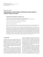
wavelet coefficients. Consider the graph of Figure 1,where
a SigShrink function is plotted in the positive half plan. Due
to the antisymmetry of the SigShrink function, we only focus
on the curvature of arc
OA.LetC be the intersection between
the abscissa axis and the tangent at point A to the curve
of the SigShrink function. The equation of this tangent is
y
= 0.25(2 + τλ)(x − λ)+0.5λ. The coordinates of point
C are C
= (τλ
2
/(2 + τλ), 0). We can easily control the arc
OA
curvature via the angle, denoted by θ,betweenvector
−−→
OA,
which is fixed, and vector
−→
CA, which is carried by the tangent
to the curve of δ
τ,λ
at point A. The larger θ, the stronger the
attenuation of the coefficients with amplitudes less than or
equal to λ.Forafixedλ, the relation between angle θ and
parameter τ is
cos θ
=
−−→
OA ·
−→
CA
−−→
OA
·
−→
CA
=
10 + τλ
5
(
20 + 4τλ + τ
2
λ
2
)
.
(3)
A
CB
O
θ
Figure 1: Graph of δ
τ,λ
in the positive half plan. The points A, B,
and C represented on this graph are such that A
= (λ, λ/2), B =
(λ,0), and C is the intersection between the abscissa axis and the
tangent to δ
τ,λ
at point A.
It easily follows from (3) that 0 <θ<arccos(
√
5/5); when
θ
= arccos(
√
5/5), then τ = +∞ and δ
τ,λ
is the hard-
thresholding function of (2). From (3), we derive that τ
=
τ(θ, λ) can be written as a function of θ and λ as follows:
τ
(
θ, λ
)
=
10
λ
sin
2
θ + 2 sin θ cos θ
5cos
2
θ −1
.
(4)
In practice, when λ is fixed, the foregoing makes it possible
to control the attenuation degree we want to impose to
the data in ]0, λ[ by choosing θ, which is rather natural,
and calculating τ according to (4). Since we can control
the shrinkage by choosing θ, δ
θ,λ
= δ
τ(θ,λ),λ
henceforth
denotes the SigShrink function where τ(θ, λ)isgivenby
(4). This interpretation of the SigShrink parameters makes
it easier to find “nice” parameters for practical applications.
Summarizing, the SigShrink computation is performed in
three steps:
(1) fix threshold λ and angle θ of the SigShrink function,
with λ>0and0<θ<arccos(
√
5/5). Keep in mind
that the larger θ, the stronger the attenuation,
(2) compute the corresponding value of τ from (4),
(3) shrink the data according to the SigShrink function
δ
τ,λ
defined by (1).
Hereafter, the terms “attenuation degree” and “thresh-
old” designate θ and λ, respectively. In addition, the notation
δ
τ,λ
will be preferred for calculations and statements. The
notation δ
θ,λ
, introduced just above, will be used for practical
and experimental purposes since the attenuation degree θ
is far more natural in practice than parameter τ.Some
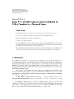
SigShrink graphs are plotted in Figure 2 for different values
of the attenuation degree θ (fixed threshold λ).
EURASIP Journal on Image and Video Processing 3
Figure 2: Shapes of SigShrink functions for different values of the
attenuation degree θ: θ
= π/6 for the continuous (blue) curve,
θ
= π/4 for the dotted (red) curve, and θ = π/3 for the dashed
(magenta) curve.
3. Sigmoid Shrinkage in the Wavelet Domain
3.1. Estimation via Shrinkage in the Wavelet Domain. Let us
recall the main principles of the nonparametric estimation
by wavelet shrinkage (the so-called WaveShrink estimation)
in the sense of [4]. Let y
={y
i
}
1iN
stand for the sequence
of noisy data y
i
= f (t
i
)+e
i
, i = 1, 2, , N,where f is
an unknown deterministic function, the random variables
{e
i
}
1iN
are independent and identically distributed (iid),
Gaussian with null mean and variance σ
2
, in short, e
i
∼
N (0, σ
2
)foreveryi = 1, 2, , N.
Inordertoestimate
{f (t
i
)}
1iN
, we assume that an
orthonormal transform, represented by an orthonormal
matrix W,isappliedtoy. The outcome of this transform is
the sequence of coefficients
c
i
= d
i
+
i
, i = 1, 2, , N,
(5)
where c
={c
i
}
1iN
= W y, d ={d
i
}
1iN
= W f, f =
{
f (t
i
)}
1iN
and ={
i
}
1iN
= W e, e ={e
i
}
1iN
.The
random variables
{
i
}
1iN
are iid and
i
∼ N (0,σ
2
). The
transform W is assumed to achieve a sparse representation
of the signal in the sense that, among the coefficients
d
i
, i = 1, 2, , N, only a few of them have large amplitudes
and, as such, characterize the signal. In this respect, simple
estimators such as “keep or kill” and “shrink or kill” rules are
proved to be nearly optimal, in the Mean Square Error (MSE)
sense, in comparison with oracles (see [4] for further details).
The wavelet transform is sparse in the sense given above
for smooth and piecewise regular signals [4]. Hereafter, the
matrix W represents an orthonormal wavelet transform.
Let
d ={δ(c
i
)}
1iN
be the sequence resulting from the
shrinkage of
{c
i
}
1iN
by using a function δ(·). We obtain an
estimate of f by setting
f = W
d where W
is the transpose,
and thus, the inverse orthonormal wavelet transform.
In [4], the hard and soft-thresholding functions are
proposed for wavelet coefficient estimation of a signal
corrupted by Additive, White and Gaussian Noise (AWGN).
Using these thresholding functions adjusted with suitable
thresholds, [4] shows that, in AWGN, the wavelet-based
estimators thus obtained achieve within a factor of 2 log N
of the performance achieved with the aid of an oracle.
Despite the asymptotic near-optimality of these standard
thresholding functions, we have the following limitations.
The hard-thresholding function is not everywhere continu-
ous and its discontinuities generate a high variance of the
estimate; on the other hand, the soft-thresholding function
is continuous but creates an attenuation on large coefficients,
which results in an over smoothing and an important bias
for the estimate [5]. In practice, these thresholding functions
(and their alternatives “nonnegative garrote” function [6],
“smoothly clipped absolute deviation” function [7]) yield
musical noise in speech denoising and visual artifacts or
over smoothing of the estimate in image processing (see,
e.g., the experimental results given in Section 4.1). Moreover,
although thresholding rules are proved to be relevant strate-
gies for estimating sparse signals [4], wavelet representations
of many signals encountered in practical applications such
as speech and image processing fail to be sparse enough
(see illustrations given in [8, Figure 3]). For a signal whose
wavelet representation fails to be sparse enough, it is more
convenient to impose the penalized shrinkage condition (P2)
instead of zero forcing since small coefficients may contain
significant information about the signal. Condition (P1)
guarantees the regularity of the shrinkage process, and the
role of condition (P3) is to avoid over smoothing of the
estimate (noise mainly affects small wavelet coefficients).
SigShrink functions are thus suitable functions for such an
estimation since they satisfy (P1), (P2), and (P3) conditions.
The following addresses the optimization of the SigShrink
parameters.
3.2. SURE-Based Optimization of SigShrink Parameters.
Consider the WaveShrink estimation described in
Section 3.1. The risk function or cost used to measure
the accuracy of a WaveShrink estimator
f of f is the standard
MSE. Since the transform W is orthonormal, this cost is
r
δ
d,
d
=
1
N
E
d −
d
2
=
1
N
N
i=1
E
(
d
i
−δ
(
c
i
))
2
(6)
for a shrinkage function δ. The SURE approach [2]involves
estimating unbiasedly the risk r
δ
(d,
d). The SURE optimiza-
tion then consists in finding the set of parameters that
minimizes this unbiased estimate. The following result is a
consequence of [3, Theorem 1].
Proposition 3.1. The quantity ϑ +
d
2
2
/N,where·
2
denotes
2
-norm and
ϑ
(
τ, λ
)
=
1
N
N
i=1
2σ
2
−c
2
i
+2
σ
2
+ σ
2
τ|c
i
|−c
2
i
e
−τ(|c
i
|−λ)
(
1+e
−τ(|c
i
|−λ)
)
2
,
(7)
is an unbiased estimator of the risk r
δ
τ,λ
(d,
d),whereδ
τ,λ
is a
SigShrink function.
4 EURASIP Journal on Image and Video Processing
Proof. From [3, Theorem 1], we have that
r
δ
d,
d
=
1
N
⎛
⎝
d
2
2
+
N
i=1
E
δ
2
(
c
i
)
−2c
i
δ
(
c
i
)
+2σ
2
δ
(
c
i
)
⎞
⎠
,
(8)
where δ can be any differentiable shrinkage function that
does not explode at infinity (see [3] for details). A SigShrink
function is such a shrinkage function. Taking into account
that the derivate of the SigShrink function δ
τ,λ
is
δ
τ,λ
(
x
)
=
1+
(
1+τ|x|
)
e
−τ(|x|−λ)
(
1+e
−τ(|x|−λ)
)
2
,
(9)
the result derives from (1), (8), and (9).
As a consequence of Proposition 3.1, we get that mini-
mizing r
δ
τ,λ
(d,
d)of(6) amounts to minimizing the unbiased
(SURE) estimator ϑ given by (7). The next section presents
experimental tests for illustrating the SURE SigShrink
denoising of some natural images corrupted by AWGN.
For every tested image and every noise standard deviation
considered, the optimal SURE SigShrink parameters are
those minimizing ϑ, the vector c representing the wavelet
coefficients of the noisy image.
3.3. Experimental Results. The SURE optimization approach
for SigShrink is now given for some standard test images cor-
rupted by AWGN. We consider the standard 2-dimensional
Discrete Wavelet Transform (DWT) by using the Symlet
wavelet of order 8 (“sym8” in the Matlab Wavelet toolbox).
The SigShrink estimation is compared with that of
the SURELET “sum of DOGs” (Derivatives Of Gaus-
sian). SURELET (free MatLab software is avalaible at
fl.ch/demo/suredenoising/)isaSURE-
based method that moreover includes an interscale predictor
with a priori information about the position of significant
wavelet coefficients. For the comparison with SigShrink,
we only use the “sum of DOGs” parameterization, that
is, the SURELET method without inter-scale predictor and
Gaussian smoothing. By so proceeding, we thus compare two
shrinkage functions: SigShrink and “sum of DOGs.”
In the sequel, the SURE SigShrink parameters (attenua-
tion degree and threshold) are those obtained by performing
the SURE optimization on the whole set of the detail
DWT coefficients. The attenuation degree and threshold
thus computed are then applied at every decomposition
level to the detail DWT coefficients. We also introduce
the SURE Level-Dependent SigShrink (SURE LD-SigShrink)
parameters. These parameters are obtained by applying
an SURE optimization at every detail (horizontal, vertical,
diagonal) subimage located at the different resolution levels
concerned (4 resolution levels in our experiments).
The tests are carried out with the following values for
the noise standard deviation: σ
= 5, 15, 25, 35. For every
value σ, 25 tests have been performed based on different
noise realizations. Every test involves performing a DWT
for the tested image corrupted by AWGN, computing the
optimal SURE parameters (SigShrink and LD-SigShrink),
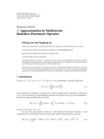
500
450
400
350
300
250
200
150
100
50
50 100 150 200 250 300 350 400 450 500
Figure 3: Noisy “Lena” image. Noise is AWGN with standard
deviation σ
= 35, which corresponds to an input PSNR =
17.2494 dB.
applying the SigShrink function with these parameters to
denoise the wavelet coefficients, and building an estimate of
the corresponding image by applying the inverse DWT to the
shrunken coefficients. For every test, the PSNR is calculated
for the original image and the denoised image. The PSNR
(in deciBel unit, dB), often used to assess the quality of a
compressed image, is given by
PSNR
= 10log
10
ν
2
MSE
, (10)
where ν stands for the dynamics of the signal, ν
= 255 in the
case of 8 bit-coded images.
Ta bl e 1 gives the following statistics for the 25 PSNRs
obtained by the SURE SigShrink, SURE LD-SigShrink, and
“sum of DOGs” method: average value, variance, minimum,
and maximum. Average values and variances for the SURE
SigShrink and SURE LD-SigShrink parameters are given in
Ta bl es 2, 3, 4,and5.
Remark 3.2. We use the Matlab routine fmincon to compute
the optimal SURE SigShrink parameters. This function
computes the minimum of a constrained multivariable
function by using nonlinear programming methods (see
Matlab help for the details). Note the following. First, one
can use a test set and average the optimal parameter values
on this set for application to images other than those used
in the test set. By so proceeding, we avoid the systematic
use of optimization algorithms such as fmincon on images
that do not pertain to the test class. The low variability that
holds among the optimal parameters given in Tables 2, 3, 4,
and 5 ensures the robustness of the average values. Second,
instead of using optimal parameters, one can use heuristic
ones (calculated by taking into account the physical meaning
of these parameters and the noise statistical properties) such
EURASIP Journal on Image and Video Processing 5
Table 1: Means, variances, minima, and maxima of the PSNRs computed over 25 noise realizations, when denoising test images by the SURE
SigShrink, SURE LD-SigShrink, and “sum of DOGs” methods. The tested images are corrupted by AWGN with standard deviation σ.The
DWT is computed by using the “sym8” wavelet. Some statistics are given in Tables 2, 3, 4,and5 for the SigShrink and LD-SigShrink optimal
SURE parameters.
Image “House” “Peppers” “Barbara” “Lena” “Flin” “Finger” “Boat” “Barco”
σ =5 (⇒ Input PSNR = 34.1514).
Mean(PSNR)
SigShrink 37.1570 36.4765 36.2587 37.3046 35.2207 35.3831 36.1187 36.6890
LD-SigShrink 37.4880 36.6827 36.3980 37.5518 35.3128 35.8805 36.3608 36.9928
SURELET 37.3752 36.6708 36.3767 37.5023 35.3102 35.9472 36.3489 35.9698
Var(PSNR) ×10
3
SigShrink 0.4269 0.3635 0.0746 0.0696 0.0702 0.0630 0.0533 0.5338
LD-SigShrink 0.8786 0.3081 0.0879 0.0643 0.0262 0.0571 0.0937 0.5613
SURELET 0.5154 0.4434 0.0994 0.1241 0.0413 0.0453 0.0479 0.3132
Min(PSNR)
SigShrink 37.1067 36.4479 36.2409 37.2837 35.2021 35.3681 36.1060 36.6384
LD-SigShrink 37.4427 36.6502 36.3764 37.5377 35.3043 35.8695 36.3409 36.9220
SURELET 37.3196 36.6280 36.3502 37.4799 35.2986 35.9355 36.3353 35.9190
Max(PSNR)
SigShrink 37.2101 36.5211 36.2753 37.3202 35.2385 35.4043 36.1309 36.7345
LD-SigShrink 37.5405 36.7100 36.4175 37.5750 35.3244 35.8985 36.3790 37.0374
SURELET 37.4218 36.7061 36.3967 37.5198 35.3255 35.9614 36.3636 35.9960
σ =15 (⇒Input PSNR = 24.6090).
Mean(PSNR)
SigShrink 31.0833 29.5395 28.9750 31.3434 27.9386 28.1546 29.6099 29.9200
LD-SigShrink 31.6472 30.0930 29.3972 32.0571 28.3815 29.4191 30.2895 30.4545
SURELET 31.2834 29.9621 29.2817 31.9059 28.3502 29.4365 30.2706 27.4525
Var(PSNR)
SigShrink 0.0016 0.0010 0.0003 0.0003 0.0001 0.0002 0.0003 0.0019
LD-SigShrink 0.0030 0.0009 0.0003 0.0008 0.0002 0.0002 0.0003 0.0015
SURELET 0.0014 0.0008 0.0003 0.0004 0.0001 0.0002 0.0003 0.0005
Min(PSNR)
SigShrink 31.0022 29.4883 28.9490 31.3068 27.9221 28.1188 29.5829 29.8443
LD-SigShrink 31.5005 30.0315 29.3741 31.9621 28.3647 29.3908 30.2563 30.3773
SURELET 31.2056 29.9124 29.2378 31.8653 28.3339 29.3967 30.2468 27.4074
Max(PSNR)
SigShrink 31.1630 29.6216 29.0129 31.3777 27.9555 28.1724 29.6416 30.0088
LD-SigShrink 31.7552 30.1848 29.4313 32.0952 28.4164 29.4604 30.3272 30.5144
SURELET 31.3555 30.0225 29.3075 31.9350 28.3616 29.4571 30.3093 27.4843
σ =25 (⇒Input PSNR = 20.1720).
Mean(PSNR)
SigShrink 28.5549 26.5452 25.9539 28.7835 24.8761 25.1774 26.9844 27.2684
LD-SigShrink 29.2948 27.3111 26.5146 29.7435 25.6407 26.6262 27.8216 27.9599
SURELET 28.8085 26.9941 26.4404 29.5937 25.5953 26.7659 27.8227 23.6221
Var(PSNR)
SigShrink 0.0015 0.0009 0.0004 0.0007 0.0002 0.0002 0.0002 0.0017
LD-SigShrink 0.0028 0.0022 0.0006 0.0013 0.0002 0.0003 0.0007 0.0024
SURELET 0.0015 0.0024 0.0004 0.0004 0.0003 0.0003 0.0004 0.0006
Min(PSNR)
SigShrink 28.4563 26.4906 25.9164 28.7256 24.8499 25.1474 26.9606 27.1534
LD-SigShrink 29.1894 27.2160 26.4642 29.6501 25.6143 26.5912 27.7927 27.8702
SURELET 28.7439 26.8867 26.4128 29.5424 25.5599 26.7256 27.7803 23.5541
Max(PSNR)
SigShrink 28.6309 26.5974 25.9921 28.8215 24.8962 25.1962 27.0133 27.3490
LD-SigShrink 29.4082 27.3887 26.5684 29.8135 25.6715 26.6726 27.8970 28.0518
SURELET 28.8828 27.0884 26.4771 29.6331 25.6259 26.8062 27.8615 23.6703
σ =35 (⇒Input PSNR = 17.2494).
Mean(PSNR)
SigShrink 26.9799 24.6863 24.2771 27.1918 22.9274 23.3429 25.4271 25.7142
LD-SigShrink 27.7840 25.5818 24.8910 28.2782 23.9326 24.9625 26.3764 26.5068
SURELET 27.2768 25.1307 24.8383 28.1462 23.8954 25.0756 26.3880 21.3570
Var(PSNR)
SigShrink 0.0018 0.0014 0.0005 0.0011 0.0002 0.0002 0.0006 0.0020
LD-SigShrink 0.0071 0.0035 0.0006 0.0022 0.0007 0.0003 0.0011 0.0035
SURELET 0.0021 0.0012 0.0004 0.0008 0.0003 0.0003 0.0006 0.0007
6 EURASIP Journal on Image and Video Processing
Table 1: Continued.
Image “House” “Peppers” “Barbara” “Lena” “Flin” “Finger” “Boat” “Barco”
Min(PSNR)
SigShrink 26.8957 24.6337 24.2299 27.1388 22.9031 23.3139 25.3856 25.6094
LD-SigShrink 27.6242 25.4966 24.8499 28.1395 23.8746 24.9369 26.3102 26.3964
SURELET 27.1928 25.0577 24.7906 28.0753 23.8608 25.0446 26.3167 21.3180
Max(PSNR)
SigShrink 27.0502 24.7740 24.3079 27.2623 22.9493 23.3813 25.4782 25.7942
LD-SigShrink 27.9473 25.7515 24.9507 28.3628 23.9717 24.9984 26.4346 26.5985
SURELET 27.3627 25.2000 24.8701 28.1867 23.9375 25.1146 26.4311 21.4116
Table 2: Mean values (based on 25 noise realizations) for optimal DWT “sym8” SURE SigShrink parameters, when denoising the “Lena”
image corrupted by AWGN. The SURE SigShrink parameters are the SigShrink parameters θ and λ obtained by performing the SURE
optimization on the whole set of the detail DWT coefficients. It follows from these results that the threshold height as well as the attenuation
degree tends to be increasing functions of the noise standard deviation σ.
Image “House” “Peppers” “Barbara” “Lena” “Flinstones” “Fingerprint” “Boat” “Barco”
σ =5
Mean θ 0.3183 0.2615 0.2655 0.3054 0.1309 0.1309 0.1913 0.3122
Mean λ/σ 2.3420 1.9289 1.9156 2.3861 1.1145 1.1375 1.6885 2.1334
σ =15
Mean θ 0.5113 0.4407 0.4256 0.5158 0.3429 0.3491 0.4264 0.4584
Mean λ/σ 3.0439 2.6016 2.6259 3.1045 2.3897 2.4181 2.8454 2.8954
σ =25
Mean θ 0.5640 0.4931 0.4638 0.5764 0.4305 0.4310 0.4997 0.5185
Mean λ/σ 3.2612 2.7893 2.9397 3.3283 2.7167 2.7670 3.1414 3.2043
σ =35
Mean θ 0.5925 0.5151 0.4900 0.6066 0.4761 0.4802 0.5389 0.5505
Mean λ/σ 3.3885 2.9240 3.2249 3.4733 2.8835 2.9493 3.3459 3.4142
as the standard minimax or universal thresholds, which are
shown to perform well with SigShrink (see Section 4).
From Tab le 1, it follows that the 3 methods yield PSNRs
of the same order. The level dependent strategy for SigShrink
(LD-SigShrink) tends to achieve better results than the
SigShrink and the “sum of DOGs.” For every method,
the difference (over the 25 noise realizations) between the
minimum and maximum PSNR is less than 0.2 dB.
From Tables 2, 3, 4,and5, we observe (concerning the
optimal SURE SigShrink parameters) that
(i) the threshold height as well as the attenuation degree
tends to be increasing functions of the noise standard
deviation σ,
(ii) for every tested σ, the SURE level-dependent attenu-
ation degree and threshold tend to decrease when the
resolution level increase (see Tabl e 4),
(iii) for every fixed σ, the variance of the optimal
SURE parameters over the 25 noise realizations is
small; optimal parameters are not very disturbed for
different noise realizations,
(iv) as far as the level dependent strategy is concerned,
the attenuation degree as well as the threshold tends
to decrease when the resolution level increases for a
fixed σ.
4. Smooth Adaptation
In this section, we highlight specific features of SigShrink
functions with respect to several issues in image processing.
Besides its simplicity (function with explicit close form,
in contrast to parametric methods such as Bayesian shrink-
ages [9–14]), the main features of the SigShrink functions in
image processing are the following.
Adjustable Denoising. The flexibility of the SigShrink param-
eters allows to choose the denoising level. From hard
denoising (degenerated SigShrink) to smooth denoising,
there exists a wide class of regularities that can be attained
for the denoised signal by adjusting the attenuation degree
and threshold.
Artifact-Free Denoising. The smoothness of the nondegener-
ated SigShrink functions allows for reducing noise without
impacting significantly the signal; a better preservation of
the signal characteristics (visual perception) and its statistical
properties is guaranteed due to the fact that the shrinkage is
performed with less variability among coefficients with close
values.
Contrast Function. The SigShrink function and its inverse,
the SigStretch function, can be seen as contrast functions.
EURASIP Journal on Image and Video Processing 7
Table 3: Variances (based on 25 noise realizations) for the optimal SURE SigShrink parameters whose means are given in Ta bl e 2.
Image “House” “Peppers” “Barbara” “Lena” “Flinstones” “Fingerprint” “Boat” “Barco”
σ =5
Var θ:10
−04
× 0.1550 0.2625 0.0877 0.0592 0.0002 0.0004 0.0642 0.2138
Var λ/σ:10
−03
× 0.0932 0.2204 0.0591 0.0209 0.0015 0.0017 0.1454 0.1500
σ =15
Var θ:10
−04
× 0.4569 0.2777 0.0468 0.1946 0.0722 0.0297 0.0478 0.5645
Var λ/σ: 0.0002 0.0001 0.0003 0.0011 0.0003 0.0003 0.0018 0.0001
σ =25
Var θ:10
−04
× 0.4858 0.3753 0.0968 0.1594 0.0433 0.0586 0.1100 0.6510
Var λ/σ:10
−03
× 0.6270 0.1439 0.0504 0.1215 0.0184 0.0227 0.0452 0.3095
σ =35
Var θ:10
−04
× 0.7011 0.3639 0.1123 0.2463 0.0662 0.1041 0.0982 0.8360
Var λ/σ:10
−03
× 0.9610 0.4325 0.1219 0.1720 0.2287 0.0445 0.1570 0.7928
Table 4: Mean values of the optimal SURE LD-SigShrink parameters, for the denoising of the “Lena” image corrupted by AWGN. The DWT
with the “sym8” wavelet is used. The SURE LD-SigShrink parameters are obtained by applying a SURE optimization at every detail (Hori.
for Horizontal, Vert. for Vertical, Diag. for Diagonal) subimage located at the differentresolutionlevelsconcerned.Weremarkfirstthatthe
threshold height, as well as the attenuation degree, tends to be increasing functions of the noise standard deviation σ. In addition, for every
σ considered, the attenuation degree as well as the threshold tends to decrease when the resolution level increases.
σ =5
θλ/σ
Hori. Vert. Diag. Hori. Vert. Diag.
J
= 1 0.2864 0.2738 0.3172 3.1072 2.3829 4.2136
J
= 2 0.2298 0.1722 0.3057 1.8747 1.4181 2.1687
J
= 3 0.0863 0.0657 0.1868 0.7361 0.4852 1.3251
J
= 4 0.1154 0.1558 0.4071 0.4957 0.4867 1.4383
σ =15
θλ/σ
Hori. Vert. Diag. Hori. Vert. Diag.
J
= 1 0.5397 0.4517 0.9361 4.9893 4.0930 4.6560
J
= 2 0.4209 0.3767 0.4641 2.9436 2.4534 3.1053
J
= 3 0.2622 0.1794 0.3481 1.9541 1.3087 2.2195
J
= 4 0.2128 0.3161 0.4528 1.0539 1.0125 1.8657
σ =25
θλ/σ
Hori. Vert. Diag. Hori. Vert. Diag.
J
= 1 0.8934 0.5412 0.9712 4.5129 5.0167 4.4367
J
= 2 0.4633 0.4217 0.5209 3.5723 2.8134 3.8653
J
= 3 0.3294 0.2642 0.4135 2.4032 1.7920 2.5764
J
= 4 0.2644 0.3264 0.4655 1.5004 1.3231 2.0720
σ =35
θλ/σ
Hori. Vert. Diag. Hori. Vert. Diag.
J
= 1 0.8772 0.8785 0.9575 4.6843 4.5268 4.6499
J
= 2 0.4963 0.4389 0.5746 4.2031 3.2062 4.5700
J
= 3 0.3643 0.2745 0.4424 2.6642 1.9881 2.8343
J
= 4 0.2700 0.3119 0.4743 1.6543 1.3744 2.2185
8 EURASIP Journal on Image and Video Processing
Table 5: Variances (based on 25 noise realizations) for optimal SURE SigShrink parameters whose means are given in Ta bl e 4.
σ =5
θλ/σ
Hori.Vert.Diag.Hori.Vert.Diag.
J
= 14.0132 ×10
−05
2.3941 ×10
−05
7.8842 ×10
−05
3.2225 ×10
−04
1.2107 ×10
−04
1.2801 ×10
−02
J =27.1936 ×10
−05
9.1042 ×10
−05
8.2755 ×10
−05
8.9961 ×10
−04
2.1122 ×10
−02
3.3873 ×10
−04
J =33.9358 ×10
−04
1.9894 ×10
−06
4.9047 ×10
−04
1.7802 ×10
−02
9.4616 ×10
−05
8.1475 ×10
−03
J =43.8724 ×10
−02
7.2803 ×10
−02
1.0830 ×10
−02
2.6745 ×10
−02
4.4741 ×10
−02
9.0581 ×10
−03
σ =15
θλ/σ
Hori.Vert.Diag.Hori.Vert.Diag.
J
= 11.1386 ×10
−05
8.5503 ×10
−05
2.9411 ×10
−02
9.1445 ×10
−04
5.2059 ×10
−03
1.7085 ×10
−01
J =21.2669 ×10
−04
1.0311 ×10
−04
1.8030 ×10
−04
3.1178 ×10
−04
3.7783 ×10
−04
1.3153 ×10
−03
J =37.0001 ×10
−04
9.6295 ×10
−04
4.0143 ×10
−03
5.8012 ×10
−03
1.7847 ×10
−02
1.1231 ×10
−03
J =43.5209 ×10
−02
8.4438 ×10
−02
4.7492 ×10
−03
6.0936 ×10
−02
1.2701 ×10
−01
5.4097 ×10
−03
σ =25
θλ/σ
Hori.Vert.Diag.Hori.Vert.Diag.
J
= 13.6502 ×10
−03
6.7723 ×10
−05
1.3148 ×10
−02
3.2220 ×10
−01
3.0924 ×10
−03
3.718 ×10
−01
J =22.2414 ×10
−04
1.5173 ×10
−04
4.5237 ×10
−04
3.7254 ×10
−03
4.2258 ×10
−04
1.5425 ×10
−02
J =35.9582 ×10
−04
2.5486 ×10
−05
4.3791 ×10
−04
2.6453 ×10
−02
8.5859 ×10
−04
8.3580 ×10
−04
J =41.0268 ×10
−04
1.8425 ×10
−02
3.0014 ×10
−02
2.9073 ×10
−02
7.6271 ×10
−03
3.6192 ×10
−03
σ =35
θλ/σ
Hori.Vert.Diag.Hori.Vert.Diag.
J
= 12.2438 ×10
−02
3.7058 ×10
−02
1.1533 ×10
−02
2.7270 ×10
−01
2.6113 ×10
−01
2.8441 ×10
−01
J =24.7551 ×10
−04
2.7514 ×10
−04
9.0224 ×10
−04
4.2308 ×10
−02
2.0487 ×10
−03
9.8234 ×10
−02
J =39.0951 ×10
−04
2.1239 ×10
−04
8.5623 ×10
−04
3.2461 ×10
−03
1.2198 ×10
−03
3.4412 ×10
−03
J =45.9373 ×10
−04
9.1487 ×10
−03
2.8074 ×10
−03
4.2265 ×10
−03
5.6180 ×10
−03
4.9168 ×10
−03
The SigShrink function enhances contrast, whereas the
SigStretch function reduces contrast.
In what follows, we detail these characteristics. The
following proposition characterizes the SigStretch function.
Proposition 4.1. The SigStretch function, denoted r
τ,λ
,is
defined as the inverse of the SigShrink function δ
τ,λ
and is given
by
r
τ,λ
(
z
)
= z +
sgn
(
z
)
L
τ|z|e
−τ(|z|−λ)
τ
(11)
for any real value z, with L being the Lambert function defined
as the inverse of the function: t 0
→ te
t
.
Proof. [See appendix].
In the rest of the paper, the wavelet transform used is the
Stationary (also call shift-invariant or redundant) Wavelet
Transform (SWT) [15]. This transform has appreciable
properties in denoising. Its redundancy makes it possible to
reduce residual noise due to the translation sensitivity of the
orthonormal wavelet transform.
4.1. Adjustable and Artifact-Free Denoising. The shrinkage
performed by the SigShrink method is adjustable via the
attenuation degree θ and the threshold λ.
Figures 4 and 5 give denoising examples for different
values of θ and λ. The denoising concerns the “Lena” image
corrupted by AWGN with standard deviation σ
= 35
(Figure 3). The “Haar” wavelet and 4 decomposition levels
are used for the wavelet representation (SWT). The classical
minimax and universal thresholds [4] are used. In these
figures, SigShrink
θ,λ
stands for the SigShrink function which
parameters are θ and λ.
For a fixed attenuation degree, we observe that the
smoother denoising is obtained with the larger threshold
(universal threshold). Small value for the threshold (mini-
max threshold) leads to better preservation of the textural
EURASIP Journal on Image and Video Processing 9
PSNR = 27.3019 dB
(a) SigShrink
π/6,λ
u
PSNR = 27.011 dB
(b) SigShrink
π/4,λ
u
PSNR = 26.8441 dB
(c) SigShrink
π/3,λ
u
PSNR = 27.2852 dB
(d) SigShrink
π/6,λ
m
PSNR = 28.1485 dB
(e) SigShrink
π/4,λ
m
PSNR = 27.944 dB
(f) SigShrink
π/3,λ
m
Figure 4: SWT SigShrink denoising of “Lena” image corrupted by AWGN with standard deviation σ = 35. The universal threshold λ
u
and the minimax threshold λ
m
are used. The universal threshold (the larger threshold) yields a smoother denoising, whereas the minimax
threshold leads to better preservation of the textural information contained in the image.
information contained in the image (compare in Figure 4,
image (a) versus image (d); image (b) versus image (e); image
(c) versus image (f); or equivalently, compare the zooms of
these images shown in Figure 5).
Now, for a fixed threshold λ, the SigShrink shape is
controllable via θ (see Figure 2). The attenuation degree
θ,0 <θ<arccos(
√
5/5), reflects the regularity of the
shrinkage and the attenuation imposed to data with small
amplitudes (mainly noise coefficients). The larger θ, the
more the noise reduction. However, SigShrink functions are
more regular for small values of θ,andthus,smallvaluesfor
θ lead to less artifacts (in Figure 5, compare images 5(d), 5(e),
and 5(f)).
It follows that SigShrink denoising is flexible thanks to
parameters λ and θ, preserves the image features, and leads
to artifact-free denoising. It is thus possible to reduce noise
without impacting the signal characteristics significantly.
Artifact free denoising is relevant in many applications, in
particular for medical imagery where visual artifacts must be
avoided. In this respect, we henceforth consider small values
for the attenuation degree.
Note that the SURELET “sum of DOGs” parameteriza-
tion does not allow for such a heuristically adjustable denois-
ing because the physical interpretation of its parameters is
not explicit, whereas the SigShrink and the standard hard,
soft, NNG, and SCAD thresholding functions mentioned
in Section 3.1 depend on parameters with more intuitive
physical meaning (threshold height and an additional atten-
uation degree parameter for SigSghink). Denoising examples
achieved by using the hard, soft, NNG, and SCAD thresh-
olding functions are given in Figure 6,foracomparisonwith
the SigShrink denoising. The minimax threshold is used for
the denoising (the results are even worse with the universal
threshold). As can be seen in this figure, artifacts are visible
in the image denoised by using hard thresholding, whereas
images denoised by using soft, NNG, and SCAD thresholding
functions tend to be over smoothed. Numerical comparison
of the denoising PSNRs performed by SigShrink and these
standard thresholding functions can be found in [1].
At this stage, it is worth mentioning the following.
Some parametric shrinkages using a priori distributions for
modeling the signal wavelet coefficients can sometimes be
10 EURASIP Journal on Image and Video Processing
PSNR = 27.3019 dB
(a) SigShrink
π/6,λ
u
PSNR = 27.011 dB
(b) SigShrink
π/4,λ
u
PSNR = 26.8441 dB
(c) SigShrink
π/3,λ
u
PSNR = 27.2852 dB
(d) SigShrink
π/6,λ
m
PSNR = 28.1485 dB
(e) SigShrink
π/4,λ
m
PSNR = 27.944 dB
(f) SigShrink
π/3,λ
m
Figure 5: Zoom of the SigShrink denoising of “Lena” images of Figure 4.
described by nonparametric functions with explicit formulas
(e.g., a Laplacian assumption leads to a soft-thresholding
shrinkage). In this respect, one can wonder about possible
links between SigShrink and the Bayesian Sigmoid Shrinkage
(BSS) of [14]. BSS is a one-parameter family of shrinkage
functions; whereas SigShrink functions depend on two
parameters. Fixing one of these two parameters yields a
subclass of SigShrink functions. It is then reasonable to
think that depending on the distribution of the signal and
noise wavelet coefficients, these functions should somehow
relate to BSS. Actually, such a possible link has not yet been
established.
To conclude this section, note that shrinkages and
regularization procedures are linked in the sense that a
shrinkage function solves to a regularization problem con-
strained by a specific penalty function [16]. Since SigShrink
functions satisfy assumptions of [16, Proposition 3.2], the
shrinkage obtained by using a function δ
τ,λ
canbeseenas
a regularization approximation [7] by seeking the vector d
that minimizes the penalized least squares
d − c
2
2
+2
N
i=1
q
τ,λ
(
|d
i
|
)
,
(12)
where q
λ
= q
τ,λ
(·) is the penalty function associated with
δ
τ,λ
, q
τ,λ
is defined for every x 0by
q
τ,λ
(
x
)
=
x
0
r
τ,λ
(
z
)
−z
dz,
(13)
with r
τ,λ
being the SigStretch function (inverse of the
SigShrink function δ
τ,λ
,see(11)). Thus, SigShrink has several
interpretations depending on the model used.
4.2. Speckle Denoising. In SAR, oceanography and medical
ultrasonic imagery, sensors record many gigabits of data per
day. These images are mainly corrupted by speckle noise.
If postprocessing such as segmentation or change detection
have to be performed on these databases, it is essential
to be able to reduce speckle noise without impacting the
signal characteristics significantly. The following illustrates
that SigShrink makes it possible to achieve this because of
its flexibility (see the shapes of SigShrink functions given in
Figure 2) and the artifact-free denoising they perform (see
Figures 4 and 5). In addition, since SigShrink is invertible, it
is not essential to store a copy of the original database (thou-
sands and thousands of gigabits recorded every year); one
can retrieve an original image by simply applying the inverse
SigShrink denoising procedure (SigStrech functions). More
EURASIP Journal on Image and Video Processing 11
Hard
λ
m
PSNR = 27.8706 dB
(a)
Soft
λ
m
PSNR = 25.2785 dB
(b)
NNG
λ
m
PSNR = 26.4129 dB
(c)
SCAD
λ
m
PSNR = 25.7867 dB
(d)
Figure 6: Denoising examples by using standard thresholding functions. The “Haar” wavelet and 4 decomposition levels are used for the
wavelet representation (SWT). The denoising concerns the image of Figure 3.
precisely, the following illustrates that SigShrink performs
well for denoising speckle noise in the wavelet domain.
Speckle noise is a multiplicative type noise inherent
to signal acquisition systems using coherent radiation.
This multiplicative noise is usually modeled as a corre-
lated stationary random process independent of the signal
reflectance.
Two d ifferent additive representations are often used
for speckle noise. The first model is a “signal-dependent”
stationary noise model; noise, assumed to be stationary,
depends on the signal reflectance. This model is simply
obtained by noting that
z = z + z( − 1), with z being
the signal reflectance and
being a stationary random
process independent of z. The second model is a “signal-
independent” model obtained by applying a logarithmic
transform to the noisy image.
We begin with the speckle signal-dependent model. The
denoising procedure then involves applying an SWT to the
noisy image, estimating the noise standard deviation in
each SWT subband by the robust Median of the Absolute
Deviation ((MAD), normalized by the constant 0.6745)
estimator [4], shrinking the wavelet coefficients by using a
SigShrink function adjusted with the minimax threshold [4],
and reconstructing an estimate of the signal by means of
the inverse SWT. The results obtained for the “Lena” image
corrupted by speckle noise (Figure 7(a)) are shown in Figures
7(b) and 7(c).
In addition, we consider the speckle signal-independent
model. We use the estimation procedure described above
for denoising the logarithmic transformed noisy image. The
results are given in Figures 7(d) and 7(e).
By comparing the results of Figure 7, we observe that
the PSNRs achieved are of the same order whatever the
model. However, the denoising obtained with the additive
independent noise model (logarithmic transform) has a
better visual quality than that obtained with the additive
signal-dependent speckle model. In fact, one can note, from
this figure, the ability of SigShrink functions to reduce
speckle noise without impacting structural features and
textural information of the image. Note also the gain in
12 EURASIP Journal on Image and Video Processing
PSNR = 29.0567 dB
(d) SigShrink
π/6,λ
m
PSNR = 29.2328 dB
(e) SigShrink
π/4,λ
m
Denoising with logarithmic transform
PSNR
= 29.0078 dB
(b) SigShrink
π/6,λ
m
PSNR = 29.4059 dB
(c) SigShrink
π/4,λ
m
Denoising without logarithmic transform
PSNR
= 18.8301 dB
(a) Noisy image
Figure 7: SigShrink denoising of the “Lena” image corrupted by speckle noise. The SWT with four resolution levels and the Haar filters are
used. The noise standard deviation is estimated by the MAD normalized by the constant 0.6745 (see [4]).
PSNR is larger than 10 dBs, performance of the same order
as that of the best up-to-date speckle denoising techniques
([17–22] among others).
4.3. Contrast Funct ion. To conclude this section, we now
present the SigShrink and SigStretch functions as contrast
functions. Contrast functions are very useful in medical
image processing. As a matter of fact, medical monitoring
for arthroplasty (replacement of certain bone surfaces by
implants due to lesions of the articular surfaces) requires 2D-
3D registration of the implant, and thus, requires knowing
exactly the position of the implant contour. Precise edge
EURASIP Journal on Image and Video Processing 13
(a) SigStretch
π/6,100
(b) Original image (c) SigShrink
π/6,100
Figure 8: SigStretch and SigShrink applied on the “Lena” image.
(a) Original image (b) SigShrink
π/6,255
(c) SigShrink
π/4,255
Figure 9: SigStretch and SigShrink applied on a fluoroscopic image.
detection is no easy task [23] because edge detection
methods are sensitive to contrast (global contrast for the
image and local contrast around a contour). The following
briefly describes how to use SigShrink-SigStretch functions
as contrast functions.
The SigShrink function applies a penalized shrinkage to
data with small amplitudes. The smaller the data ampli-
tude, the higher the attenuation imposed by the SigShrink
function. Thus, a SigShrink function is a contrast enhancing
function; this function increases the gap between large and
small values for the pixels of an image. As a consequence,
a SigStretch function reduces the contrast by lowering the
variation between large and small pixel values in the image.
Figure 8 gives the original “Lena” image as well as the
SigShrink δ
π/6,100
and SigStretch r
π/6,100
shrunken images.
This figure highlights that the contrast of the image can
be smoothly adjusted (enhancement, reduction) by applying
SigShrink and SigStretch functions without introducing
artifacts. Note that, as for denoising, SigShrink allows for
choosing the attenuation degree imposed to the data, when
the threshold height is fixed. Figure 9 illustrates the variabil-
ity that can be attained by varying the SigShrink attenuation
degree for enhancing the contrast of a fluoroscopic image.
To conclude this section, we now illustrate the combina-
tion of SigShrink denoising and contrast enhancement for an
ultrasonic image of breast cancer. The combination involves
denoising the image by using the SigShrink method in the
wavelet domain. A SigShrink function is then applied to
the denoised image to enhance its contrast. The results are
presented in Figure 10. It is shown that SigShrink denoises
the image and preserves feature information without intro-
ducing artifacts. The parameter θ
= π/6 is chosen so as to
avoid visual artifacts. Different thresholds are experimented
to highlight how we can progressively reduce noise without
affecting the image textural information. The threshold λ
d
is
the detection threshold of [8]. This threshold is smaller than
the minimax threshold. It is close to λ
u
/2 when the sample
size is large.
14 EURASIP Journal on Image and Video Processing
SigShrink denoising combined with SigShrink
π/6,100
contrast enhancement
(a) Ultrasonic image
(b) SigShrink
π/6,λ
d
(c) SigShrink
π/6,λ
m
(d) SigShrink
π/6,λ
u
(e) SigShrink
π/6,λ
d
(f) SigShrink
π/6,λ
m
(g) SigShrink
π/6,λ
u
SigShrink denoising without contrast enhancement
Figure 10: SigShrink denoising for an ultrasonic image of breast cancer. The SWT with four resolution levels and the biorthogonal spline
wavelet with order 3 for decomposition and with order 1 for reconstruction (“bior1.3” in Matlab Wavelet toolbox) are used. The noise
standard deviation is estimated by the MAD normalized by the constant 0.6745 (see [4]).
5. Conclusion
This work proposes the use of SigShrink-SigStretch functions
for practical engineering problems such as image denoising,
image restoration, and image enhancement. These functions
perform adjustable adaptation of data in the sense that
they can enhance or reduce the variability among data, the
adaptation process being regular and invertible. Because of
the smoothness of the function used (infinitely differentiable
in ]0, +
∞[), the data adaptation is performed with little vari-
ability so that the signal characteristics are better preserved.
The SigShrink and SigStretch methods are simple and flexible
EURASIP Journal on Image and Video Processing 15
in the sense that the parameters of these classes of functions
allow for a fine tuning of the data adaptation. This adaptation
is nonparametric because no prior information about the
signal is taken into account. A SURE-based optimization of
the parameters is possible.
The denoising achieved by a SigShrink function is almost
artifact-free due to the little variability introduced among
data with close amplitudes. This artifact-free denoising is
relevant for many applications, in particular for medical
imagery where visual artifacts must be avoided. In addition,
a fine calibration of SigShrink parameters allows noise
reduction without impacting the signal characteristics. This
is important when some postprocessing (such as a segmen-
tation) must be performed on the signal estimate.
As far as perspectives are concerned, we can reasonably
expect to improve SigShrink denoising performance by
introducing interscale or/and intrascale predictor, which
could provide information about the position of significant
wavelet coefficients. It could also be relevant to undertake a
complete theoretical and experimental comparison between
SigShrink and Bayesian sigmoid shrinkage [14].
In addition, application of SigShrink to speech process-
ing could also be considered. Since SigShrink yields denoised
images that are almost artifact-free, would it be possible
that such an approach denoises speech signals corrupted
by AWGN without returning musical noise, in contrast to
classical shrinkages using thresholding rules?
Another perspective is the SigShrink-SigStretch calibra-
tion of contrast in order to improve edge detection in
medical imagery. Exact edge detection is necessary for 2D-
3D registration of images. Subpixel measurement of edge is
possible by using, for example, the moment-based method of
[24]. However, the method is very sensible to contrast. Low
contrast varying images result in multiple contours; whereas
high varying contrast in image leads to good precision for
certain contour points but induces lack of detection for
points in lower contrast zones. The idea is the use of the
SigShrink-SigStretch functions for improving image contrast
so as to alleviate edge detection in medical imagery. For
instance, we can expect that combining SigShrink-SigStretch
with edge detection methods such as [24] can lead to good
subpixel measurement of the contour in an image.
Appendix
Proof of Proposition 4.1
Because δ
τ,λ
is antisymmetric, r
τ,λ
has the form
r
τ,λ
(
z
)
= zG
(
z
)
,
(A.1)
for every real value z and where G is such that
G
(
z
)
= 1+e
−τ(|z|G(z)−λ)
.
(A.2)
Therefore, G(z) > 1 for any real value z.Wethushave
(
G
(
z
)
−1
)
e
τ(|z|
(
G
(
z
)
−1
)
)
= e
−τ(|z|−λ)
,
(A.3)
which is also equivalent to
τ
|z|
(
G
(
z
)
−1
)
e
τ(|z|
(
G
(
z
)
−1
)
)
= τ|z|e
−τ(|z|−λ)
.
(A.4)
It follows that
τ
|z|
(
G
(
z
)
−1
)
= L
τ|z|e
−τ(|z|−λ)
,(A.5)
which leads to
G
(
z
)
= 1+
L
τ|z|e
−τ(|z|−λ)
(
τ
|z|
)
(A.6)
for z
/
=0. The result then follows from (A.1), (A.6), and the
fact that r
τ,λ
(0) = 0 since δ
τ,λ
(0) = 0.
References
[1] A. M. Atto, D. Pastor, and G. Mercier, “Smooth sigmoid
wavelet shrinkage for non-parametric estimation,” in Proceed-
ings of the IEEE International Conference on Acoustics, Speech
and Signal Processing (ICASSP ’08), pp. 3265–3268, Las Vegas,
Nev, USA, March-April 2008.
[2] C. Stein, “Estimation of the mean of a multivariate normal
distribution,” The Annals of Statistics, vol. 9, pp. 1135–1151,
1981.
[3] F. Luisier, T. Blu, and M. Unser, “A new sure approach to image
denoising: interscale orthonormal wavelet thresholding,” IEEE
Transactions on Image Processing, vol. 16, no. 3, pp. 593–606,
2007.
[4] D. L. Donoho and I. M. Johnstone, “Ideal spatial adaptation
by wavelet shrinkage,” Biometrika, vol. 81, no. 3, pp. 425–455,
1994.
[5] A. G. Bruce and H Y. E. Gao, “Understanding waveshrink:
variance and bias estimation,” Biometrika,vol.83,no.4,pp.
727–745, 1996.
[6] H Y. Gao, “Wavelet shrinkage denoising using the non-
negative garrote,” Journal of Computational and Graphical
Statistics, vol. 7, no. 4, pp. 469–488, 1998.
[7] A. Antoniadis and J. Fan, “Regularization of wavelet approx-
imations,” Journal of the American Statistical Association, vol.
96, no. 455, pp. 939–955, 2001.
[8] E. P. Simoncelli and E. H. Adelson, “Noise removal via
bayesian wavelet coring,” in Proceedings of the IEEE Interna-
tional Conference on Image Processing (ICIP ’96), vol. 1, pp.
379–382, Lausanne, Switzerland, September 1996.
[9]M.N.DoandM.Vetterli,“Wavelet-basedtextureretrieval
using generalized Gaussian density and Kullback-Leibler dis-
tance,” IEEE Transactions on Image Processing,vol.11,no.2,
pp. 146–158, 2002.
[10] L. S¸endur and I. W. Selesnick, “Bivariate shrinkage functions
for wavelet-based denoising exploiting interscale dependency,”
IEEE Transactions on Signal Processing, vol. 50, no. 11, pp.
2744–2756, 2002.
[11] J. Portilla, V. Strela, M. J. Wainwright, and E. P. Simoncelli,
“Image denoising using scale mixtures of Gaussians in the
wavelet domain,” IEEE Transactions on Image Processing, vol.
12, no. 11, pp. 1338–1351, 2003.
[12] I. M. Johnstone and B. W. Silverman, “Empirical bayes
selection of wavelet thresholds,” Annals of Statistics, vol. 33, no.
4, pp. 1700–1752, 2005.
[13] C. J. F. ter Braak, “Bayesian sigmoid shrinkage with improper
variance priors and an application to wavelet denoising,”
Computational Statistics and Data Analysis,vol.51,no.2,pp.
1232–1242, 2006.
[14] R. R. Coifman and D. L. Donoho, Translation Invariant de-
Noising, Lecture Notes in Statistics, Springer, New York, NY,
USA, 1995.
16 EURASIP Journal on Image and Video Processing
[15] H. Xie, L. E. Pierce, and F. T. Ulaby, “SAR speckle reduction
using wavelet denoising and markov random field modeling,”
IEEE Transactions on Geoscience and Remote Sensing, vol. 40,
no. 10, pp. 2196–2212, 2002.
[16] F. Argenti and L. Alparone, “Speckle removal from SAR images
in the undecimated wavelet domain,” IEEE Transactions on
Geoscience and Remote Sensing, vol. 40, no. 11, pp. 2363–2374,
2002.
[17] A. Achim, P. Tsakalides, and A. Bezerianos, “SAR image
denoising via bayesian wavelet shrinkage based on heavy-
tailed modeling,” IEEE Transactions on Geoscience and Remote
Sensing, vol. 41, no. 8, pp. 1773–1784, 2003.
[18] F. Argenti, T. Bianchi, and L. Alparone, “Multiresolution
MAP despeckling of SAR images based on locally adaptive
generalized Gaussian pdf modeling,” IEEE Transactions on
Image Processing, vol. 15, no. 11, pp. 3385–3399, 2006.
[19] A. Achim, E. E. Kuruoglu, and J. Zerubia, “SAR image filtering
based on the heavy-tailed Rayleigh model,” IEEE Transactions
on Image Processing, vol. 15, no. 9, pp. 2686–2693, 2006.
[20] D. Sen, M. N. S. Swamy, and M. O. Ahmad, “Computationally
fast techniques to reduce AWGN and speckle in videos,” IET
Image Processing, vol. 1, no. 4, pp. 319–334, 2007.
[21] A. Antoniadis, “Wavelet methods in statistics: some recent
developments and their applications,” Statistics Surveys, vol. 1,
pp. 16–55, 2007.
[22] M. R. Mahfouz, W. A. Hoff, R. D. Komistek, and D. A. Dennis,
“Effect of segmentation errors on 3D-to-2D registration of
implant models in X-ray images,” Journal of Biomechanics, vol.
38, no. 2, pp. 229–239, 2005.
[23]A.M.Atto,D.Pastor,andG.Mercier,“Detectionthreshold
for non-parametric estimation,” Signal, Image and Video
Processing, vol. 2, no. 3, pp. 207–223, 2008.
[24] E.P.Lyvers,O.R.Mitchell,M.L.Akey,andA.P.Reeves,“Sub-
pixel measurements using a moment-based edge operator,”
IEEE Transactions on Pattern Analysis and Machine Intelligence,
vol. 11, no. 12, pp. 1293–1309, 1989.