báo cáo hóa học:" Research Article Database of Multichannel In-Ear and Behind-the-Ear Head-Related and Binaural Room Impulse Responses" ppt
Bạn đang xem bản rút gọn của tài liệu. Xem và tải ngay bản đầy đủ của tài liệu tại đây (7.41 MB, 10 trang )
Hindawi Publishing Corporation
EURASIP Journal on Advances in Signal Processing
Volume 2009, Article ID 298605, 10 pages
doi:10.1155/2009/298605
Research Article
Database of Multichannel In-Ear and Behind-the-Ear
Head-Related and Binaural Room Impulse Responses
H.Kayser,S.D.Ewert,J.Anem
¨
uller, T. Rohdenburg, V. Hohmann, and B. Kol lmeier
Medizinische Physik, Universit
¨
at Oldenburg, 26111 Oldenburg, Germany
Correspondence should be addressed to H. Kayser,
Received 15 December 2008; Accepted 4 June 2009
Recommended by Hugo Fastl
An eight-channel database of head-related impulse responses (HRIRs) and binaural room impulse responses (BRIRs) is
introduced. The impulse responses (IRs) were measured with three-channel behind-the-ear (BTEs) hearing aids and an in-ear
microphone at both ears of a human head and torso simulator. The database aims at providing a tool for the evaluation of
multichannel hearing aid algorithms in hearing aid research. In addition to the HRIRs derived from measurements in an anechoic
chamber, sets of BRIRs for multiple, realistic head and sound-source positions in four natural environments reflecting daily-
life communication situations with different reverberation times are provided. For comparison, analytically derived IRs for a
rigid acoustic sphere were computed at the multichannel microphone positions of the BTEs and differences to real HRIRs were
examined. The scenes’ natural acoustic background was also recorded in each of the real-world environments for all eight channels.
Overall, the present database allows for a realistic construction of simulated sound fields for hearing instrument research and,
consequently, for a realistic evaluation of hearing instrument algorithms.
Copyright © 2009 H. Kayser et al. This is an open access article distributed under the Creative Commons Attribution License,
which permits unrestricted use, distribution, and reproduction in any medium, provided the original work is properly cited.
1. Introduction
Performance evaluation is an important part of hearing
instrument algorithm research since only a careful evaluation
of accomplished effects can identify truly promising and
successful signal enhancement methods. The gold standard
for evaluation will always be the unconstrained real-world
environment, which comes however at a relatively high cost
in terms of time and effort for performance comparisons.
Simulation approaches to the evaluation task are the
first steps in identifying good signal processing algorithms.
It is therefore important to utilize simulated input signals
that represent real-world signals as faithfully as possible,
especially if multimicrophone arrays and binaural hearing
instrument algorithms are considered that expect input from
both sides of a listener’s head. The simplest approach to
model the input signals to a multichannel or binaural hearing
instrument is the free-field model. More elaborate models
are based on analytical formulations of the effect that a rigid
sphere has on the acoustic field [1, 2].
Finally, the synthetic generation of multichannel input
signals by means of convolving recorded (single-channel)
sound signals with impulse responses (IRs) corresponding
to the respective spatial sound source positions, and also
depending on the spatial microphone locations, represents a
good approximation to the expected recordings from a real-
world sound field. It comes at a fraction of the cost and with
virtually unlimited flexibility in arranging different acoustic
objects at various locations in virtual acoustic space if the
appropriate room-, head-, and microphone-related impulse
responses are available.
In addition, when recordings from multichannel hearing
aids and in-ear microphones in a real acoustic background
sound field are available, even more realistic situations can be
produced by superimposing convolved contributions from
localized sound sources with the approximately omnidirec-
tional real sound field recording at a predefined mixing ratio.
By this means, the level of disturbing background noise
can be controlled independently from the localized sound
sources.
Under the assumption of a linear and time-invariant
propagation of sound from a fixed source to a receiver,
the impulse response completely describes the system. All
transmission characteristics of the environment and objects
2 EURASIP Journal on Advances in Signal Processing
in the surrounding area are included. The transmission of
sound from a source to human ears is also described in
this way. Under anechoic conditions the impulse response
contains only the influence of the human head (and torso)
and therefore is referred to as head-related impulse response
(HRIR). Its Fourier transform is correspondingly referred
to as head-related transfer function (HRTF). Binaural head-
related IRs recorded in rooms are typically referred to as
binaural room impulse responses (BRIRs).
There are several existing free available databases con-
taining HRIRs or HRTFs measured on individual subjects
and different artificial head-and-torso simulators (HATS)
[3–6]. However these databases are not suitable to simulate
sound impinging on hearing aids located behind the ears
(BTEs) as they are limited to two-channel information
recorded near the entrance of the ear canal. Additionally the
databases do not reflect the influence of the room acoustics.
For the evaluation of modern hearing aids, which
typically process 2 or 3 microphone signals per ear, multi-
channel input data are required corresponding to the real
microphone locations (in the case of BTE devices behind the
ear and outside the pinna) and characterizing the respective
room acoustics.
The database presented here therefore improves over
existing publicly available data in two respects: In contrast to
other HRIR and BRIR databases, it provides a dummy-head
recording as well as an appropriate number of microphone
channel locations at realistic spatial positions behind the ear.
In addition, several room acoustical conditions are included.
Especially for the application in hearing aids, a broad set
of test situations is important for developing and testing of
algorithms performing audio processing. The availability of
multichannel measurements of HRIRs and BRIRs captured
by hearing aids enables the use of signal processing tech-
niques which benefit from multichannel input, for example,
blind source separation, sound source localization and
beamforming. Real-world problems, such as head shading
and microphone mismatch [7] can be considered by this
means.
A comparison between the HRTFs derived from the
recorded HRIRs at the in-ear and behind-the-ear positions
and respective modeled HRTFs based on a rigid spherical
head is presented to analyze deviations between simulations
and a real measurements. Particularly at high frequencies,
deviations are expected related to the geometric differences
between the real head including the pinnae and the model’s
spherical head.
The new database of head-, room- and microphone-
related impulse responses, for convenience consistently
referred to as HRIRs in the following, contains six-channel
hearing aid measurements (three per side) and additionally
the in-ear HRIRs measured on a Br
¨
uel & Kjær HATS [8]in
different environments.
After a short overview of the measurement method and
setup, the acoustic situations contained in the database are
summarized, followed by a description of the analytical
head model and the methods used to analyze the data.
Finally, the results obtained under anechoic conditions are
compared to synthetically generated HRTFs based on the
7.3
7.6
13.6
2.1
2.6
32.7
4
4
4
34
5
5
5
6
6
Figure 1: Right ear of the artificial head with a hearing aid dummy.
The distances between the microphones of the hearing aids and the
entrance to the earcanal on the artificial head are given in mm.
model of a rigid sphere. The database is available under
/>2. Methods
2.1. Acoustic Setup. Data was recorded using the head-and-
torso simulator Br
¨
uel & Kjær Type 4128C onto which the BTE
hearing aids were mounted (see Figure 1). The use of a HATS
has the advantage of a fixed geometry and thereby provides
highly reproducible acoustic parameters. In addition to the
microphones in the BTEs mounted on the HATS, it also
provides internal microphones to record sound pressure near
the location corresponding to the place of the human ear
drum.
The head-and-torso simulator was used with artificial
ears Br
¨
uel & Kjær Type 4158C (right) and Type 4159C
(left) including preamplifiers Type 2669. Recordings were
carried out with the in-ear microphones and two three-
channel BTE hearing aid dummies of type Acuris provided
by Siemens Audiologische Technik GmbH, one behind each
artificial ear, resulting in a total of 8 recording channels. The
term “hearing aid dummy” refers to the microphone array
of a hearing aid, housed in its original casing but without
any of the integrated amplifiers, speakers or signal processors
commonly used in hearing aids.
EURASIP Journal on Advances in Signal Processing 3
The recorded analog signals were preamplified
using a G.R.A.S. Power Module Type 12AA, with the
amplification set to +20 dB (in-ear microphones) and a
Siemens custom-made pre-amplifier, with an amplification
of +26 dB on the hearing aid microphones. Signals
were converted using a 24-bit multichannel AD/DA-
converter (RME Hammerfall DSP Multiface) connected
to a laptop (DELL Latitude 610D, Pentium M processor
@1.73 Ghz,1 GB RAM) via a PCMCIA-card and the digital
data was stored either on the internal or an external
hard disk. The software used for the recordings was
MATLAB (MathWorks, Versions 7.1/7.2, R14/R2006a) with
a professional tool for multichannel I/O and real-time
processing of audio signals (SoundMex2 [9]).
The measurement stimuli for measuring a HRIR were
generated digitally on the computer using MATLAB-
scripts (developed in-house) and presented via the AD/DA-
converter to a loudspeaker. The measurement stimuli were
emitted by an active 2-channel coaxial broadband loud-
speaker (Tannoy 800A LH). All data was recorded at a
sampling rate of 48 kHz and stored at a resolution of 32 Bit.
2.2. HRIR Measurement. The HRIR measurements were
carried out for a variety of natural recording situations.
Some of the scenarios were suffering from relatively high
levels of ambient noise during the recording. Additionally,
at some recording sites, special care had to be taken of
the public (e.g., cafeteria). The measurement procedure
was therefore required to be of low annoyance while the
measurement stimuli had to be played back at a sufficient
level and duration to satisfy the demand of a high signal-
to-noise ratio imposed by the use of the recorded HRIRs
for development and high-quality auralization purposes.
To meet all requirements, the recently developed modified
inverse-repeated sequence (MIRS) method [10]wasused.
The method is based on maximum length sequences (MLS)
which are highly robust against transient noise since their
energy is distributed uniformly in the form of noise over the
whole impulse response [11]. Furthermore, the broadband
noise characteristics of MLS stimuli made them suitable
for presentation in the public rather than, for example,
sine-sweep stimuli-based methods [12]. However, MLSs are
known to be relatively sensitive to (even weak) nonlinearities
in the measurement setup. Since the recordings at public sites
required partially high levels reproduced by small scale and
portable equipment, the risk of non-linear distortions was
present. Inverse repeated sequences (IRS) are a modification
to MLSs which show high robustness against even-order
nonlinear distortions [13]. An IRS consists of two concate-
nated MLS s(n) and its inverse:
IRS
(
n
)
=
⎧
⎨
⎩
s
(
n
)
, n even,
−s
(
n
)
, n odd,
0
≤ n ≤ 2L,(1)
where L is the period of the generating MLS. The IRS
therefore has a period of 2L. In the MIRS method employed
here, IRSs of different orders are used in one measurement
process and the resulting impulse responses of different
lengths are median-filtered to further suppress the effect
of uneven-order nonlinear distortions after the following
scheme: A MIRS consists of several successive IRS of different
orders. In the evaluation step, the resulting periodic IRs of
the same order were averaged yielding a set of IRs of different
orders. The median of these IRs was calculated and the final
IR was shortened to length corresponding to the lowest order.
The highest IRS order in the measurements was 19, which is
equal to a length of 10.92 seconds at the used sampling rate
of 48 kHz. The overall MIRS was 32.77 seconds in duration
and the calculated raws IRs were 2.73 seconds corresponding
to 131072 samples.
The MIRS method combines the advantages of MLS
measurements with high immunity against non-linear dis-
tortions. A comparison of the measurement results to an
efficient method proposed by Farina [12] showed that the
MIRS technique achieves competitive results in anechoic
conditions with regard to signal-to-noise ratio and was better
suited in public conditions (for details see [10]).
The transfer characteristics of the measurement system
was not compensated for in the HRIRs presented here,
since it does not effect the interaural and microphone
array differences. The impulse response of the loudspeaker
measured by a probe microphone at the HATS position in
the anechoic chamber is provided as part of the database.
2.3. Content of the Database. A summary of HRIR mea-
surements and recordings of ambient acoustic backgrounds
(noise) is found in Ta bl e 1.
2.3.1. Anechoic Chamber. To simulate a nonreverberant
situation, the measurements were conducted in the anechoic
chamber of the University of Oldenburg. The HATS was
fixed on a computer-controlled turntable (Br
¨
uel & KjærType
5960C w ith Controller Type 5997) and placed opposite to the
speaker in the room as shown in Figure 2. Impulse responses
were measured for distances of 0.8 m and 3 m between
speaker and the HATS. The larger distance corresponds to
a far-field situation (which is, e.g., commonly required by
beam-forming algorithms) whereas for the smaller distance
near-field effects may occur. For each distance, 4 angles of
elevation were measured ranging from
−10
◦
to 20
◦
in steps
of 10
◦
. For each elevation the azimuth angle of the source to
the HATS was varied from 0
◦
(front) to −180
◦
(left turn) in
steps of 5
◦
(cf. Figure 3). Hence, a total of 296 (= 37×4 ×2)
sets of impulse responses were measured.
2.3.2. Office I. In an office room at the University of
Oldenburg similar measurements were conducted, covering
the systematic variation of the sources’ spatial positions. The
HATS was placed on a desk and the speaker was moved in
the front hemisphere (from
−90
◦
to +90
◦
) at a distance of
1 m with an elevation angle of 0
◦
. The step size of alteration
of the azimuth angle was 5
◦
as for the anechoic chamber.
For this environment only the BTE channels were
measured.
A detailed sketch of the recording setup for this and the
other environments is provided as a part of the database.
4 EURASIP Journal on Advances in Signal Processing
Table 1: Summary of all measurements of head related impulse responses and recordings of ambient noise. In the Office I environment
(marked by the asterisk) only the BTE channels were measured.
Environment HRIR sets measured Sounds recorded
Anechoic chamber 296 —
Office I 37
∗
—
Office II 8 12 recordings of ambient noise, total duration 19 min
Cafeteria 12 2 recordings of ambient noise, total duration 14 min
Courtyard 12 1 recording of ambient noise, total duration 24 min
Total 365 57 min of different ambient noises
Figure 2: Setup for the impulse response measurement in the
anechoic room. Additional damping material was used to cover the
equipment in the room in order to avoid undesired reflections.
20
◦
10
◦
0
◦
−10
◦
0
◦
−90
◦
90
◦
(−)180
◦
Figure 3: Coordinate systems for elevation angles (left-hand
sketch) and azimuth angles (right-hand sketch).
2.3.3. Office II. Further measurements and recordings were
carried out in a different office room of similar size.
The head-and-torso simulator was positioned on a chair
behind a desk with two head orientations of 0
◦
(looking
straight ahead) and 90
◦
(looking over the shoulder). Impulse
responses were measured for four different speaker positions
(entrance to the room, two different desk conditions and
one with a speaker standing at the window) to allow
for simulation of sound sources at typical communication
positions. For measurements with the speaker positioned at
the entrance the door was opened and for the measurement
at the window this was also open. For the remaining
measurements door and window were closed to reduce
disturbing background noise from the corridor and from
outdoors. In total, this results in 8 sets of impulse responses.
Separate recordings of real office ambient sound sources
were performed: a telephone ringing (30 seconds recorded
for each head orientation) and keyboard typing at the other
office desks (3 minutes recorded for each head orientation).
The noise emitted by the ventilation, which is installed in the
ceiling, was recorded for 5 minutes (both head orientations).
Additionally, the sound of opening and closing the door was
recorded 15 times.
2.3.4. Cafeteria. 12 sets of impulse responses were measured
in the fully occupied cafeteria of the natural sciences campus
of the University of Oldenburg. The HATS was used to
measure the impulse responses from different positions and
to collect ambient sound signals from the cafeteria. The busy
lunch time hour was chosen to obtain realistic conditions.
The ambient sounds consisted mainly of unintelligible
babble of voices from simultaneous conversations all over
the place, occasional parts of intelligible speech from nearby
speakers and the clanking of dishes and chairs scratching on
the stone floor.
2.3.5. Courtyard. Measurements in the courtyard of the
natural sciences campus of the University of Oldenburg
were conducted analogous to the Office II and Cafeteria
recordings described above. A path for pedestrians and
bicycles crosses this yard. The ambient sounds consist of
snippets of conversation between people passing by, foot
steps and mechanical sounds from bicycles including sudden
events such as ringing and squeaking of brakes. Continuous
noise from trees and birds in the surrounding was also
present.
2.4. Analytical Model and Data Analysis Methods. The char-
acteristics of HRIRs and the corresponding HRTFs originates
from diffraction, shading and resonances on the head and on
the pinnae [14]. Also reflections and diffractions of the sound
from the torso influence the HRTFs.
An analytical approximative model of the sound prop-
agation around the head is the scattering of sound by a
rigid sphere whose diameter a equals the diameter of a
human head. This is a simplification as the shoulders and the
EURASIP Journal on Advances in Signal Processing 5
pinnae are neglected and the head is regarded as spherically
symmetric.
The solution in the frequency domain for the diffraction
of sound waves on a sphere traces back to Lord Rayleigh
[15] in 1904. He derived the transfer function H(
∞, θ, μ)
dependent on the normalized frequency μ
= ka = 2πfa/c
(c: sound velocity) for an infinitely distant source impinging
at the angle θ between the surface normal at the observation
point and the source:
H
∞, θ, μ
=
1
μ
2
∞
m=0
(
−i
)
m−1
(
2m +1
)
P
m
(
cos θ
)
h
m
μ
,(2)
where P
m
denotes the Legendre polynomials, h
m
the mth-
order spherical Hankel function and h
m
its derivative.
Rabinowitz et al. [16] presented a solution for a point source
in the distance r from the center of the sphere:
H
r, θ, μ
=−
r
aμ
e
−iμr/a
Ψ,(3)
with
Ψ
=
∞
m=0
(
2m +1
)
P
m
(
cos θ
)
h
m
μr/a
h
m
μ
, r>α. (4)
2.4.1. Calculation of Binaural Cues. The binaural cues,
namely the interaural level difference (ILD), the interaural
phase difference (IPD) and derived therefrom the interaural
time difference (ITD), can be calculated in the frequency
domain from a measured or simulated HRTF [17]. If
H
l
(α, ϕ, f ) denotes the HRTF from the source to the left
ear and H
r
(α, ϕ, f ) the transmission to the right ear, the
interaural transfer function (ITF) is given by
ITF
α, ϕ, f
=
H
l
α, ϕ, f
H
r
α, ϕ, f
,(5)
with α and ϕ the azimuth and elevations angles, respectively,
as shown in Figure 3 and f representing the frequency in Hz.
The ILD is determined by
ILD
α, ϕ, f
= 20 · log
10
ITF
α, ϕ, f
. (6)
The IPD can also be calculated from the ITF. Derivation with
respect to the frequency f yields the ITD which equals the
group delay between both ears:
IPD
α, ϕ, f
=
arg
ITF
α, ϕ, f
,
ITD
α, ϕ, f
=−
1
2π
d
df
IPD
α, ϕ, f
.
(7)
Kuhn presented the limiting cases for (2)in[2]. For low
frequencies corresponding to the case ka
1 the transfer
function of the spherical head model simplifies to
H
lf
∞
, θ, μ
≈
1 − i
3
2
μ cos θ. (8)
This yields an angle of incidence independent ILD of 0 dB
and an angle dependent IPD. In the coordinate system given
in Figure 3 the IPD amounts to
IPD
lf
(
α
)
≈ 3ka sin α,(9)
which results in
ITD
lf
(
α
)
≈
6πa
c
sin α. (10)
For high frequencies the propagation of the waves is
described as “creeping waves” traveling around the sphere
with approximately the speed of sound. In this case, the ITD
can be derived from geometric treatment by the difference
between the distance from the source to the left ear and the
right ear considering the path along the surface of the sphere
[18]:
ITD
hf
≈
2πa
c
(
sin
(
α
)
+ α
)
. (11)
With the approximation α
≈ sin α, (tolerating an error of
5.5% for α
= 135
◦
and an error of 11% for α = 150
◦
[2]) (11)
yields:
ITD
hf
(
α
)
≈
4πa
c
sin α, (12)
which equals 2/3 times the result of (10).
In practice, the measured IPD is contaminated by noise.
Hence, the data was preprocessed before the ITD was
determined. First, the amplitude of the ITF was equalized to
unity by calculating the sign of the complex valued ITF:
ITF
α, ϕ, f
=
sign
ITF
α, ϕ, f
=
ITF
α, ϕ, f
ITF
α, ϕ, f
.
(13)
The result was then smoothed applying a sliding average
with a 20-samples window. The ITD was obtained for a
specific frequency by calculating the weighted mean of the
ITD (derived from the smoothed IPD) for a chosen range
around this frequency. As weighting function the coherence
function γ was used, respectively a measure for the coherence
γ
n
which is obtained from
γ
n
=
ITF(α, ϕ, f )
n
smoothed
. (14)
The function was raised to the power of n to control the
strength of suppression of data with a weak coherence. In the
analysis n
= 6 turned out to be a suitable choice.
3. Results
3.1. Quality of the Measurements. As evaluation of the
quality, the signal-to-noise ratio (SNR) of the measured
impulse responses was calculated for each environment. The
average noise power was estimated from the noise floor
6 EURASIP Journal on Advances in Signal Processing
ir
noise
(t) for the interval T
end
at end of the measured IR,
where the IR has declined below the noise level. The duration
of the measured IRs was sufficient to assume that only noise
was present in this part of the measured IR. With the average
power estimated for the entire duration T
= 2.73 s of the
measured IR, ir(t), the SNR was calculated as
SNR
= 10 log
10
ir
2
(t)
T
ir
2
noise
(t)
T
end
, (15)
where
· denotes the temporal average.
The results are given in Tab le 2.
3.2. Reverberation Time of the Different Environments. The
reverberation time T
60
denotes the time that it takes for the
signal energy to decay by 60 dB after the playback of the
signal is stopped. It was estimated from a room impulse
response of duration T employing the method of Schroeder
integration [19]. In the Schroeder integration, the energy
decay curve (EDC) is obtained by reverse-time integration
of the squared impulse response:
EDC
(
t
)
= 10 log
10
T
t
ir
2
(
τ
)
dτ
T
0
ir
2
(
τ
)
dτ
. (16)
The noise contained in the measured IR is assumed to spread
equally over the whole measured IR and thus leads to a
linearly decreasing offset in the EDC. A correction for the
noise is introduced by fitting a linear curve to the pure
noise energy part at the end of the EDC, where the IR has
vanished. Subsequently the linear curve, representing the
effect of noise, is subtracted from the EDC yielding the pure
IR component.
Generally, an exponential decay in time is expected and
the decay rate was found by fitting an exponential curve
to the computed decay of energy [20]. An example EDC is
shown in Figure 4. The first steeply sloped part of the curve
results from the decay of the energy of direct sound (early
decay) fading at about 0.1 seconds to the part resulting from
the diffuse reverberation tail of the IR. An exponential curve
is fitted (linear in semilogarithmic presentation) to the part
of the EDC corresponding to the reverberation tail. The T
60
time is then determined from the fitted decay curve. The
estimated T
60
times of the different environments are given
in Ta bl e 3.
3.3. Comparison to the Analytical Model of A Rigid Sphere.
Duda and Martens provide pseudocode for the evaluation
of (3) for the calculation of angle- and range-dependent
transfer functions of a sphere in [1]. The behavior of the
theoretical solution was also explored in detail within their
work and compared to measurements carried out on a
bowling ball. The pseudocode was implemented in MATLAB
and 8-channel HRTFs were calculated for the microphone
positions corresponding to the entrances of the ear canals
of the HATS and the positions of the BTE hearing aid
microphones on the artificial head.
In the following analysis, the measured HRTFs (obtained
from the measured HRIRs) are compared to the data
−40
−30
−20
−10
0
Energy level (dB)
0 0.1 0.2 0.3 0.4 0.5 0.6
Time (s)
Figure 4: Energy decay curve calculated using the method of
Schroeder integration from a impulse response of the cafeteria
(solid) and linear fit (dashed) to estimate the reverberation time
T
60
.
Table 2: Mean SNR values of the impulse response measurements
in the different environments.
Environment SNR (dB)
Anechoic chamber 104.8
Office II 94.7
Cafeteria 75.6
Courtyard 86.1
Table 3: Reverberation time of the different environments.
Environment T
60
(ms)
Anechoic chamber <50
(1)
Office II 300
Cafeteria 1250
Courtyard 900
(1)
The reverberation time estimate is limited by decay of the impulse
response of the vented loudspeaker system with a cut-off frequency of about
50 Hz.
modeled for a rigid sphere and also differences between
the in-ear HRTFs and the BTE hearing aids HRTFs are
considered. It is analyzed to which extend a spherical head
model is suitable to describe the sound incidence to the BTE
hearing aids regarding binaural cues and properties in the
time domain. The HRTFs from the anechoic room for the
distance of 3 m and an elevation angle of 0
◦
are compared to
the predictions of the model for a rigid sphere. The measured
results displayed in the figures were smoothed to obtain a
more articulate presentation. For this purpose, the HRTFs
were filtered using a sliding rectangular window with a 1/12-
octave width.
Figure 5 shows exemplary transfer functions obtained for
an azimuth angle of
−45
◦
. On the left side, the measured
HRTFs are shown, on the right side the theoretical curves for
a spherical head without torso. These were calculated for the
microphone positions corresponding to the measurement
setup as shown in Figure 1, whereby only the azimuth angles
were taken into account and the slight differences in elevation
were neglected. In the low-frequency range up to 1 kHz,
the dotted curves on the left and the right side have a
similar course except for a stronger ripple of the measured
EURASIP Journal on Advances in Signal Processing 7
−20
−10
0
10
20
Level (dB)
0.1 1 10
Frequency (kHz)
In-ear and hearing aids
(a)
−20
−10
0
10
20
Level (dB)
0.1 1 10
Frequency (kHz)
Headmodel
(b)
Figure 5: Measured HRTFs (a) (log-magnitude) from the in-ear (dashed) and the hearing aid microphones (solid) and corresponding log-
magnitude transfer functions calculated by the model for an ideal rigid sphere (b). The angle of incidence is
−45
◦
. The set of the upper
four curves display the HRTFs from the left side of the artificial head, the lower set is obtained from the right side. The light colored lines
represent the front hearing aid microphones and the dark lines the rearmost ones. A level of 0 dB corresponds to the absence of head-effects.
data. Level differences due to the transmission characteristics
of the small hearing aid microphones (solid lines) which
strongly deviates from a flat course are observed.
In the middle frequency range, both sides are still
correlated, but the characteristic notches and maxima are
much more prominent in the measurements. The intersec-
tion points of the separate curves remain similar, but the
variation of the level and the level differences between the
microphones are much stronger. The results of the in-ear
measurements show a raise of 10 dB to 15 dB in comparison
to the theoretical levels, due to resonances in the ear canal.
Above 7 kHz, effects like shadowing and resonance from
the structure of the head which are not present in the head
model have a strong influence.
In the following, the ITDs and ILDs obtained from the
measurements are examined in more detail.
3.3.1. ILD. The ILDs from the inner ear microphones and
one pair of the hearing aid microphones are shown in
Figure 6 for a subset of azimuth angles (solid lines) along
with the according curves obtained from the model (dashed
lines).
As indicated in the previous figure, the measurements
and the model show a similar behavior up to a frequency
of about 3 kHz. Above this value, the influence of the head
and the torso become obvious resulting in a strong ripple
especially for the inner ear measurements which include also
the effects of the pinnae and the ear canals.
Above a frequency of 9 kHz, alignment errors and
microphone mismatch become obvious. This is indicated
by the deviation of the ILD from the 0 dB line for sound
incidence from 0
◦
and −180
◦
.
For the ILDs of the in-ear measurements it is obvious that
the measured ILD is much bigger than the model ILD for
sound incidence from the front left side (
−30
◦
to −90
◦
)in
the frequency range above 4 kHz. If the sound impinges from
behind, notches are observable at 3 kHz for
−120
◦
and at
nearly 4 kHz at
−150
◦
in the measured ILD when compared
to the model ILD. This effect is not present in the ILDs
between the hearing aids and therefore must originate from
the pinnae.
3.3.2. ITD. The ITDs between the in-ear microphones and
a microphone pair of the hearing aids were calculated as
described in Section 2.4.1 within a range of
±100 Hz to the
center frequency. The results are shown in Figure 7,where
the modeled data is also displayed.
For center frequencies of 125 Hz and 250 Hz, the curves
obtained from the measurements and the model are in
good accordance. Above, for 0.5 kHz and 1 kHz, deviations
occur. Here, the ITDs calculated from the measurements are
slightly higher than the theoretical values for the sphere. The
determination of the azimuth angle is always ambiguous for
a sound coming from the back or the front hemisphere. For
the 2-kHz curve, the ITD becomes also ambiguous for sound
waves coming from the same hemisphere.
Another difference between the ILD for low and high
frequencies is observable. For the lower frequencies, the time
differences are larger than for higher frequencies at the same
angle of incidence, corresponding to a larger effective head
radius for low frequencies. This is in accordance with the
findings of Kuhn [2] for an infinitely distant source described
by (10)and(12).
3.3.3. Analysis in the Time Domain. Figure 8 shows HRIRs
for a sound source impinging to the left side of the HATS.
The angle of incidence ranges from 0
◦
to 360
◦
and, in
this representation, is related to the angle of incidence to
8 EURASIP Journal on Advances in Signal Processing
−180
−150
−120
−90
−60
−30
0
Azimuth angle (
◦
)
ILD (dB)
0.1 1 10
Frequency (kHz)
In-ear
(a)
−180
−150
−120
−90
−60
−30
0
Azimuth angle (
◦
)
ILD (dB)
0.1 1 10
Frequency (kHz)
Hearing aids
(b)
Figure 6: ILDs calculated from the measurements (solid lines) and the modeled HRTFs (dashed lines) for the in-ear microphones (a) and
the front microphone pair of the hearing aids (b). One tick on the right ordinate corresponds to 6 dB level difference. The dashed straight
lines mark the ILD of 0 dB.
0
0.25
0
0.25
0
0.25
0
0.25
0
0.25
0.5
0.75
1
ITD (ms)
125
250
500
1000
2000
Frequency (Hz)
−180 −150 −120 −90 −60 −30 0
Azimuth angle (
◦
)
In-ear
(a)
0
0.25
0
0.25
0
0.25
0
0.25
0
0.25
0.5
0.75
1
ITD (ms)
125
250
500
1000
2000
Frequency (Hz)
−180 −150 −120 −90 −60 −30 0
Azimuth angle (
◦
)
Hearing aids
(b)
Figure 7: ITDs calculated from the measurements (solid lines) and the modeled HRTFs (dashed lines) for the in-ear microphones (a) and
the front microphone pair of the hearing aids (b). The ITDs for the mid frequencies in octaves from 125 Hz to 2 kHz are shown as indicated
on the right-hand ordinate axis. An offset of 0.5 milliseconds is added to separate the curves from each other for a better overview. One tick
on the left-hand ordinate is 0.25 milliseconds.
the microphones on the left side of the head for a better
overview.Thismeans,foranangleof0
◦
, the sound impinges
perpendicularly to the hearing aid. The set of HRIRs is
shown for the head model (a), the corresponding foremost
hearing aid microphone on the left side (b) and the left in-
ear microphone (c).
The data from the head model show a decreasing mag-
nitude of the main peak with increasing angle of incidence
up to 170
◦
. For sound incidence from the opposite direction
a peak is visible-the so-called “bright spot” which was also
described by Duda and Martens [1].
The impulse responses of the hearing aid microphone
also show a bright spot for sound incidence from 180
◦
.The
shape of the maximum peak formation is similar to the
modeled data, but after the main peak additional delayed
reflections occur. Early reflections are from the rim of the
pinna as the delay lies within the range of travel time
according to a distance of a few centimeters. A later dominant
peak is attributed to strong reflections from the shoulders as
it occurs 0.3 milliseconds to 0.5milliseconds after the main
peak which corresponds to a distance of about 13 cm to 20
cm.
For the in-ear microphones these reflections are much
morepronouncedandhaveafinerstructure.Abrightspot
is not apparent due to the asymmetry caused by the pinnae.
EURASIP Journal on Advances in Signal Processing 9
0
◦
60
◦
120
◦
180
◦
240
◦
300
◦
360
◦
Headmodel
0 0.3 0.6 0.9 1.2 1.5 1.8
Tr av el ti me ( m s)
(a)
0
◦
60
◦
120
◦
180
◦
240
◦
300
◦
360
◦
Hearing aid
0 0.3 0.6 0.9 1.2 1.5 1.8
Tr av el ti me ( m s)
(b)
0
◦
60
◦
120
◦
180
◦
240
◦
300
◦
360
◦
In-ear
0 0.3 0.6 0.9 1.2 1.5 1.8
Tr av el ti me ( m s)
(c)
Figure 8: Head-related impulse responses for sound incidence to
the left side of the artificial head. Data are shown for the head model
(a), a hearing aid microphone (b) and the left in-ear microphone
(c).
4. Discussion and Conclusion
A HRIR database was introduced, which is suited to simulate
different acoustic environments for digital sound signal
processing in hearing aids. A high SNR of the impulse
responses was achieved even under challenging real-world
recording conditions. In contrast to existing freely available
databases, six-channel measurements of BTE hearing aids
are included in addition to the in-ear HRIRs for a variety
of source positions in a free-field condition and in differ-
ent realistic reverberant environments. Recordings of the
ambient sounds characteristic to the scenes are available
separately. This allows for a highly authentic simulation of
the underlying acoustic scenes.
The outcome of the analysis of the HRTFs from the
anechoic room is in agreement with previous publications on
HRTFs (e.g., [2]) and shows noticeable differences between
the in-ear measurements and the data from the hearing aids.
As expected, the ILDs derived from the spherical head model
match the data from the hearing aids better than the data
from the in-ear measurements. The modeled ILD fits the
ILD between the hearing aids reasonably up to a frequency
of 6 kHz. For the in-ear ILD, the limit is about 4 kHz.
In the frequency region above 4 to 6 kHz significant
deviations of the simulated data and the measurements
occur. This shows, that modeling a head by a rigid sphere
does not provide a suitable estimation of sound transmission
to the microphone arrays in a BTE hearing aid and motivates
the use of this database in hearing aid research, particularly
for future hearing aids with extended frequency range.
It is expected that the data presented here will pre-
dominantly be used in the context of evaluation of signal
processing algorithms with multi-microphone input such
as beamformers or binaural algorithms. In such cases, very
detailed knowledge about magnitude and phase behavior of
the HRTFs might have to be provided as a-priori knowledge
into signal processing algorithms. Even though the current
HRTF data represent a “snapshot” of a single geometric head
arrangement that would need to be adjusted to subjects on
an individual basis, it can nevertheless be used as one specific
realization to be accounted for in certain algorithms.
It is impossible to determine a-priori whether
the detailed acoustic properties captured by realistic
HRIRs/HRTFs are indeed significant for either evaluation
or algorithm construction. However, the availability of the
current database makes it possible to answer this question for
each specific algorithm, acoustic situation and performance
measure individually. Results from work based on our
data [21] demonstrate that even for identical algorithms
and spatial arrangements, different measures can show a
significant performance increase (e.g., SNR enhancement)
when realistic HRTFs are taken into account. Conversely,
other measures (such as the speech reception threshold
under binaural conditions) have been found to be largely
invariant to the details captured by realistic models. In any
case, the availability of the HRIR database presented here
makes it possible to identify the range of realistic conditions
10 EURASIP Journal on Advances in Signal Processing
under which an arbitrary hearing instrument algorithm
performs well.
This “test-bed” environment also permits detailed com-
parison between different algorithms and may lead to a
realistic de facto standard benchmark dataset for the hearing
aid research community. The database is available under
/>Acknowledgment
The authors would like to thank Siemens Audiologische
Technik for providing the hearing aids and the appropriate
equipment. This work was supported by the DFG (SFB/TR
31) and the European Commission under the integrated
project DIRAC (Detection and Identification of Rare Audio-
visual Cues, IST-027787).
References
[1] R. O. Duda and W. L. Martens, “Range dependence of the
response of a spherical head model,” The Journal of the
Acoustical Society of America, vol. 104, no. 5, pp. 3048–3058,
1998.
[2] G. F. Kuhn, “Model for the interaural time differences in
the azimuthal plane,” TheJournaloftheAcousticalSocietyof
America, vol. 62, no. 1, pp. 157–167, 1977.
[3] V. R. Algazi, R. O. Duda, D. M. Thompson, and C. Avendano,
“The CIPIC HRTF database,” in IEEE ASSP Workshop on
Applications of Signal Processing to Audio and Acoustics, pp. 99–
102, October 2001.
[4] B. Gardner, K. Martin, et al., “HRTF measurements of a
KEMAR dummy-head microphone,” Tech. Rep. 280, MIT
Media Lab Perceptual Computing, May 1994.
[5] S. Takane, D. Arai, T. Miyajima, K. Watanabe, Y. Suzuki, and
T. Sone, “A database of head-related transfer functions in
whole directions on upper hemisphere,” Acoustical Science and
Technology, vol. 23, no. 3, pp. 160–162, 2002.
[6] H. Sutou, “Shimada laboratory HRTF database,” Tech.
Rep., Shimada Labratory, Nagaoka University of Technology,
Nagaoka, Japan, May 2002, />[7] H. Puder, “Adaptive signal processing for interference cancel-
lation in hearing aids,” Signal Processing,vol.86,no.6,pp.
1239–1253, 2006.
[8] “Head and Torso Simulator(HATS)—Type 4128,” Br
¨
uel &
Kjær, Nærum, Denmark.
[9] D. Berg, SoundMex2,H
¨
orTech gGmbH, Oldenburg, Germany,
2001.
[10] S. D. Ewert and H. Kayser, “Modified inverse repeated
sequence,” in preparation.
[11] D. D. Rife and J. Vanderkooy, “Transferfunction measurement
with maximum-lengthsequences,” Journal of Audio Engineer-
ing Society, vol. 37, no. 6, pp. 419–444, 1989.
[12] A. Farina, “Simultaneous measurement of impulse response
and distortion with a swept-sine technique,” in AES 108th
Convention, Paris, France, February 2000.
[13] C. Dunn and M. Hawksford, “Distorsion immunity of mls-
derived impulse response measurements,” Journal of Audio
Engineering Society, vol. 41, no. 5, pp. 314–335, 1993.
[14] J. Blauert, R
¨
aumliches H
¨
oren, Hirzel Verlag, 1974.
[15] L. Rayleigh and A. Lodge, “On the acoustic shadow of a
sphere,” Proceedings of the Royal Society of London, vol. 73, pp.
65–66, 1904.
[16] W. M. Rabinowitz, J. Maxwell, Y. Shao, and M. Wei, “Sound
localization cues for a magnified head: implications from
sound diffraction about a rigid sphere,” Presence, vol. 2, no.
2, pp. 125–129, 1993.
[17] J. Nix and V. Hohmann, “Sound source localization in
real sound fields based on empirical statistics of interaural
parameters,” The Journal of the Acoustical Society of America,
vol. 119, no. 1, pp. 463–479, 2006.
[18] R. S. Woodworth and H. Schlosberg, Woodworth and Schlos-
berg’s Experimental Psychology, Holt, Rinehardt and Winston,
New York, NY, USA, 1971.
[19] M. R. Schroeder, “New method of measuring reverberation
time,” The Journal of the Acoustical Society of America, vol. 36,
no. 3, pp. 409–413, 1964.
[20] M. Karjalainen and P. Antsalo, “Estimation of modal decay
parameters from noisy response measurements,” in AES 110th
Convention, Amsterdam, The Netherlands, May 2001.
[21] T. Rohdenburg, S. Goetze, V. Hohmann, K D. Kammeyer,
and B. Kollmeier, “Objective perceptual quality assessment
for self-steering binaural hearing aid microphone arrays,”
in Proceedings of IEEE International Conference on Acoustics,
Speech, and Signal Processing (ICASSP ’08), pp. 2449–2452, Las
Vegas, Nev, USA, March-April 2008.