Description Data Mining Techniques For Marketing_2 pdf

470643 c06.qxd 3/8/04 11:12 AM Page 176
176 Chapter 6
claims were paid automatically. The results were startling: The model was 100
percent accurate on unseen test data. In other words, it had discovered the
exact rules used by Caterpillar to classify the claims. On this problem, a neural
network tool was less successful. Of course, discovering known business rules
may not be particularly useful; it does, however, underline the effectiveness of
decision trees on rule-oriented problems.
Many domains, ranging from genetics to industrial processes really do have
underlying rules, though these may be quite complex and obscured by noisy
data. Decision trees are a natural choice when you suspect the existence of
underlying rules.
Measuring the Effectiveness Decision Tree
The effectiveness of a decision tree, taken as a whole, is determined by apply-
ing it to the test set—a collection of records not used to build the tree—and
observing the percentage classified correctly. This provides the classification
error rate for the tree as a whole, but it is also important to pay attention to the
quality of the individual branches of the tree. Each path through the tree rep-
resents a rule, and some rules are better than others.
At each node, whether a leaf node or a branching node, we can measure:
■■ The number of records entering the node
■■ The proportion of records in each class
■■ How those records would be classified if this were a leaf node
■■ The percentage of records classified correctly at this node
■■ The variance in distribution between the training set and the test set
Of particular interest is the percentage of records classified correctly at this
node. Surprisingly, sometimes a node higher up in the tree does a better job of
classifying the test set than nodes lower down.
Tests for Choosing the Best Split
A number of different measures are available to evaluate potential splits. Algo-
rithms developed in the machine learning community focus on the increase in

purity resulting from a split, while those developed in the statistics commu-
nity focus on the statistical significance of the difference between the distribu-
tions of the child nodes. Alternate splitting criteria often lead to trees that look
quite different from one another, but have similar performance. That is
because there are usually many candidate splits with very similar perfor-
mance. Different purity measures lead to different candidates being selected,
but since all of the measures are trying to capture the same idea, the resulting
models tend to behave similarly.
470643 c06.qxd 3/8/04 11:12 AM Page 177
Decision Trees 177
Purity and Diversity
The first edition of this book described splitting criteria in terms of the decrease
in diversity resulting from the split. In this edition, we refer instead to the
increase in purity, which seems slightly more intuitive. The two phrases refer to
the same idea. A purity measure that ranges from 0 (when no two items in the
sample are in the same class) to 1 (when all items in the sample are in the same
class) can be turned into a diversity measure by subtracting it from 1. Some of
the measures used to evaluate decision tree splits assign the lowest score to a
pure node; others assign the highest score to a pure node. This discussion
refers to all of them as purity measures, and the goal is to optimize purity by
minimizing or maximizing the chosen measure.
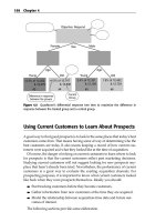
Figure 6.5 shows a good split. The parent node contains equal numbers of
light and dark dots. The left child contains nine light dots and one dark dot.
The right child contains nine dark dots and one light dot. Clearly, the purity
has increased, but how can the increase be quantified? And how can this split
be compared to others? That requires a formal definition of purity, several of
which are listed below.
Figure 6.5 A good split on a binary categorical variable increases purity.
470643 c06.qxd 3/8/04 11:12 AM Page 178
178 Chapter 6

Purity measures for evaluating splits for categorical target variables include:
■■ Gini (also called population diversity)
■■ Entropy (also called information gain)
■■ Information gain ratio
■■ Chi-square test
When the target variable is numeric, one approach is to bin the value and use
one of the above measures. There are, however, two measures in common
use for numeric targets:
■■ Reduction in variance
■■ F test
Note that the choice of an appropriate purity measure depends on whether
the target variable is categorical or numeric. The type of the input variable does
not matter, so an entire tree is built with the same purity measure. The split
illustrated in 6.5 might be provided by a numeric input variable (AGE > 46) or
by a categorical variable (STATE is a member of CT, MA, ME, NH, RI, VT). The
purity of the children is the same regardless of the type of split.
Gini or Population Diversity
One popular splitting criterion is named Gini, after Italian statistician and
economist, Corrado Gini. This measure, which is also used by biologists and
ecologists studying population diversity, gives the probability that two items
chosen at random from the same population are in the same class. For a pure
population, this probability is 1.
The Gini measure of a node is simply the sum of the squares of the propor-
tions of the classes. For the split shown in Figure 6.5, the parent population has
an equal number of light and dark dots. A node with equal numbers of each of
2 classes has a score of 0.5
2
+ 0.5
2
= 0.5, which is expected because the chance of

picking the same class twice by random selection with replacement is one out
of two. The Gini score for either of the resulting nodes is 0.1
2
+ 0.9
2
= 0.82. A
perfectly pure node would have a Gini score of 1. A node that is evenly bal-
anced would have a Gini score of 0.5. Sometimes the scores is doubled and
then 1 subtracted, so it is between 0 and 1. However, such a manipulation
makes no difference when comparing different scores to optimize purity.
To calculate the impact of a split, take the Gini score of each child node and
multiply it by the proportion of records that reach that node and then sum the
resulting numbers. In this case, since the records are split evenly between
the two nodes resulting from the split and each node has the same Gini score,
the score for the split is the same as for either of the two nodes.
470643 c06.qxd 3/8/04 11:12 AM Page 179
Decision Trees 179
Entropy Reduction or Information Gain
Information gain uses a clever idea for defining purity. If a leaf is entirely pure,
then the classes in the leaf can be easily described—they all fall in the same
class. On the other hand, if a leaf is highly impure, then describing it is much
more complicated. Information theory, a part of computer science, has devised
a measure for this situation called entropy. In information theory, entropy is a
measure of how disorganized a system is. A comprehensive introduction to
information theory is far beyond the scope of this book. For our purposes, the
intuitive notion is that the number of bits required to describe a particular sit-
uation or outcome depends on the size of the set of possible outcomes. Entropy
can be thought of as a measure of the number of yes/no questions it would
take to determine the state of the system. If there are 16 possible states, it takes
log

2
(16), or four bits, to enumerate them or identify a particular one. Addi-
tional information reduces the number of questions needed to determine the
state of the system, so information gain means the same thing as entropy
reduction. Both terms are used to describe decision tree algorithms.
The entropy of a particular decision tree node is the sum, over all the classes
represented in the node, of the proportion of records belonging to a particular
class multiplied by the base two logarithm of that proportion. (Actually, this
sum is usually multiplied by –1 in order to obtain a positive number.) The
entropy of a split is simply the sum of the entropies of all the nodes resulting
from the split weighted by each node’s proportion of the records. When
entropy reduction is chosen as a splitting criterion, the algorithm searches for
the split that reduces entropy (or, equivalently, increases information) by the
greatest amount.
For a binary target variable such as the one shown in Figure 6.5, the formula
for the entropy of a single node is
-1 * ( P(dark)log
2
P(dark) + P(light)log
2
P(light) )
In this example, P(dark) and P(light) are both one half. Plugging 0.5 into the
entropy formula gives:
-1 * (0.5 log
2
(0.5) + 0.5 log
2
(0.5))
The first term is for the light dots and the second term is for the dark dots,
but since there are equal numbers of light and dark dots, the expression sim-

plifies to –1 * log
2
(0.5) which is +1. What is the entropy of the nodes resulting
from the split? One of them has one dark dot and nine light dots, while the
other has nine dark dots and one light dots. Clearly, they each have the same
level of entropy. Namely,
-1 * (0.1 log
2
(0.1) + 0.9 log
2
(0.9)) = 0.33 + 0.14 = 0.47
470643 c06.qxd 3/8/04 11:12 AM Page 180
180 Chapter 6
To calculate the total entropy of the system after the split, multiply the
entropy of each node by the proportion of records that reach that node and
add them up to get an average. In this example, each of the new nodes receives
half the records, so the total entropy is the same as the entropy of each of the
nodes, 0.47. The total entropy reduction or information gain due to the split is
therefore 0.53. This is the figure that would be used to compare this split with
other candidates.
Information Gain Ratio
The entropy split measure can run into trouble when combined with a splitting
methodology that handles categorical input variables by creating a separate
branch for each value. This was the case for ID3, a decision tree tool developed
by Australian researcher J. Ross Quinlan in the nineteen-eighties, that became
part of several commercial data mining software packages. The problem is that
just by breaking the larger data set into many small subsets , the number of
classes represented in each node tends to go down, and with it, the entropy. The
decrease in entropy due solely to the number of branches is called the intrinsic
information of a split. (Recall that entropy is defined as the sum over all the

branches of the probability of each branch times the log base 2 of that probabil-
ity. For a random n-way split, the probability of each branch is 1/n. Therefore,
the entropy due solely to splitting from an n-way split is simply n * 1/n log
(1/n) or log(1/n). Because of the intrinsic information of many-way splits,
decision trees built using the entropy reduction splitting criterion without any
correction for the intrinsic information due to the split tend to be quite bushy.
Bushy trees with many multi-way splits are undesirable as these splits lead to
small numbers of records in each node, a recipe for unstable models.
In reaction to this problem, C5 and other descendents of ID3 that once used
information gain now use the ratio of the total information gain due to a pro-
posed split to the intrinsic information attributable solely to the number of
branches created as the criterion for evaluating proposed splits. This test
reduces the tendency towards very bushy trees that was a problem in earlier
decision tree software packages.
Chi-Square Test
As described in Chapter 5, the chi-square (X
2
) test is a test of statistical signifi-
cance developed by the English statistician Karl Pearson in 1900. Chi-square is
defined as the sum of the squares of the standardized differences between the
expected and observed frequencies of some occurrence between multiple disjoint
samples. In other words, the test is a measure of the probability that an
observed difference between samples is due only to chance. When used to
measure the purity of decision tree splits, higher values of chi-square mean
that the variation is more significant, and not due merely to chance.
470643 c06.qxd 3/8/04 11:12 AM Page 181
Decision Trees 181
first proposed split is 0.1
2
+ 0.9

2
this is also the score for the split.
Gini
right
= (4/14)
2
+ (10/14)
2
= 0.082 + 0.510 = 0.592
and the Gini score for the split is:
(6/20)Gini
left
+ (14/20)Gini
right
= 0.3*1 + 0.7*0.592 = 0.714
split that yields two nearly pure children over the split that yields one
(continued)
COMPARING TWO SPLITS USING GINI AND ENTROPY
Consider the following two splits, illustrated in the figure below. In both cases,
the population starts out perfectly balanced between dark and light dots with
ten of each type. One proposed split is the same as in Figure 6.5 yielding two
equal-sized nodes, one 90 percent dark and the other 90 percent light. The
second split yields one node that is 100 percent pure dark, but only has 6 dots
and another that that has 14 dots and is 71.4 percent light.
Which of these two proposed splits increases purity the most?
EVALUATING THE TWO SPLITS USING GINI
As explained in the main text, the Gini score for each of the two children in the
= 0.820. Since the children are the same size,
What about the second proposed split? The Gini score of the left child is 1
since only one class is represented. The Gini score of the right child is

Since the Gini score for the first proposed split (0.820) is greater than for the
second proposed split (0.714), a tree built using the Gini criterion will prefer the
completely pure child along with a larger, less pure one.
470643 c06.qxd 3/8/04 11:12 AM Page 182
182 Chapter 6
(continued)
is pure and so has entropy of 0. As for the right child, the formula for entropy is
-(P(dark)log
2
P(dark) + P(light)log
2
P(light))
so the entropy of the right child is:
Entropy
right
= -((4/14)log
2
(4/14) + (10/14)log
2
(10/14)) = 0.516 +
0.347 = 0.863
resulting nodes. In this case,
0.3*Entropy
left
+ 0.7*Entropy
right
= 0.3*0 + 0.7*0.863 = 0.604
Subtracting 0.604 from the entropy of the parent (which is 1) yields an
marketing offers.
COMPARING TWO SPLITS USING GINI AND ENTROPY

EVALUATING THE TWO SPLITS USING ENTROPY
As calculated in the main text, the entropy of the parent node is 1. The entropy
of the first proposed split is also calculated in the main text and found to be
0.47 so the information gain for the first proposed split is 0.53.
How much information is gained by the second proposed split? The left child
The entropy of the split is the weighted average of the entropies of the
information gain of 0.396. This is less than 0.53, the information gain from the
first proposed split, so in this case, entropy splitting criterion also prefers the
first split to the second. Compared to Gini, the entropy criterion does have a
stronger preference for nodes that are purer, even if smaller. This may be
appropriate in domains where there really are clear underlying rules, but it
tends to lead to less stable trees in “noisy” domains such as response to
For example, suppose the target variable is a binary flag indicating whether
or not customers continued their subscriptions at the end of the introductory
offer period and the proposed split is on acquisition channel, a categorical
variable with three classes: direct mail, outbound call, and email. If the acqui-
sition channel had no effect on renewal rate, we would expect the number of
renewals in each class to be proportional to the number of customers acquired
through that channel. For each channel, the chi-square test subtracts that
expected number of renewals from the actual observed renewals, squares the
difference, and divides the difference by the expected number. The values for
each class are added together to arrive at the score. As described in Chapter 5,
the chi-square distribution provide a way to translate this chi-square score into
a probability. To measure the purity of a split in a decision tree, the score is
sufficient. A high score means that the proposed split successfully splits the
population into subpopulations with significantly different distributions.
The chi-square test gives its name to CHAID, a well-known decision tree
algorithm first published by John A. Hartigan in 1975. The full acronym stands
for Chi-square Automatic Interaction Detector. As the phrase “automatic inter-
action detector” implies, the original motivation for CHAID was for detecting

TEAMFLY

Team-Fly
®

470643 c06.qxd 3/8/04 11:12 AM Page 183
Decision Trees 183
statistical relationships between variables. It does this by building a decision

tree, so the method has come to be used as a classification tool as well. CHAID
makes use of the Chi-square test in several ways—first to merge classes that do
not have significantly different effects on the target variable; then to choose a
best split; and finally to decide whether it is worth performing any additional
splits on a node. In the research community, the current fashion is away from
methods that continue splitting only as long as it seems likely to be useful and
towards methods that involve pruning. Some researchers, however, still prefer
the original CHAID approach, which does not rely on pruning.
The chi-square test applies to categorical variables so in the classic CHAID
algorithm, input variables must be categorical. Continuous variables must be
binned or replaced with ordinal classes such as high, medium, low. Some cur-
rent decision tree tools such as SAS Enterprise Miner, use the chi-square test
for creating splits using categorical variables, but use another statistical test,
the F test, for creating splits on continuous variables. Also, some implementa-
tions of CHAID continue to build the tree even when the splits are not statisti-
cally significant, and then apply pruning algorithms to prune the tree back.
Reduction in Variance
The four previous measures of purity all apply to categorical targets. When the
target variable is numeric, a good split should reduce the variance of the target
variable. Recall that variance is a measure of the tendency of the values in a
population to stay close to the mean value. In a sample with low variance,
most values are quite close to the mean; in a sample with high variance, many
values are quite far from the mean. The actual formula for the variance is the
mean of the sums of the squared deviations from the mean. Although the
reduction in variance split criterion is meant for numeric targets, the dark and
light dots in Figure 6.5 can still be used to illustrate it by considering the dark
dots to be 1 and the light dots to be 0. The mean value in the parent node is
clearly 0.5. Every one of the 20 observations differs from the mean by 0.5, so
the variance is (20 * 0.5
2

) / 20 = 0.25. After the split, the left child has 9 dark
spots and one light spot, so the node mean is 0.9. Nine of the observations dif-
fer from the mean value by 0.1 and one observation differs from the mean
value by 0.9 so the variance is (0.92 + 9 * 0.12) / 10 = 0.09. Since both nodes
resulting from the split have variance 0.09, the total variance after the split is
also 0.09. The reduction in variance due to the split is 0.25 – 0.09 = 0.16.
F Test
Another split criterion that can be used for numeric target variables is the F test,
named for another famous Englishman—statistician, astronomer, and geneti-
cist, Ronald. A. Fisher. Fisher and Pearson reportedly did not get along despite,
or perhaps because of, the large overlap in their areas of interest. Fisher’s test
470643 c06.qxd 3/8/04 11:12 AM Page 184
184 Chapter 6
does for continuous variables what Pearson’s chi-square test does for categori-
cal variables. It provides a measure of the probability that samples with differ-
ent means and variances are actually drawn from the same population.
There is a well-understood relationship between the variance of a sample
and the variance of the population from which it was drawn. (In fact, so long
as the samples are of reasonable size and randomly drawn from the popula-
tion, sample variance is a good estimate of population variance; very small
samples—with fewer than 30 or so observations—usually have higher vari-
ance than their corresponding populations.) The F test looks at the relationship
between two estimates of the population variance—one derived by pooling all
the samples and calculating the variance of the combined sample, and one
derived from the between-sample variance calculated as the variance of the
sample means. If the various samples are randomly drawn from the same
population, these two estimates should agree closely.
The F score is the ratio of the two estimates. It is calculated by dividing the
between-sample estimate by the pooled sample estimate. The larger the score,
the less likely it is that the samples are all randomly drawn from the same

population. In the decision tree context, a large F-score indicates that a pro-
posed split has successfully split the population into subpopulations with
significantly different distributions.
Pruning
As previously described, the decision tree keeps growing as long as new splits
can be found that improve the ability of the tree to separate the records of the
training set into increasingly pure subsets. Such a tree has been optimized for
the training set, so eliminating any leaves would only increase the error rate of
the tree on the training set. Does this imply that the full tree will also do the
best job of classifying new datasets? Certainly not!
A decision tree algorithm makes its best split first, at the root node where
there is a large population of records. As the nodes get smaller, idiosyncrasies
of the particular training records at a node come to dominate the process. One
way to think of this is that the tree finds general patterns at the big nodes and
patterns specific to the training set in the smaller nodes; that is, the tree over-
fits the training set. The result is an unstable tree that will not make good
predictions. The cure is to eliminate the unstable splits by merging smaller
leaves through a process called pruning; three general approaches to pruning
are discussed in detail.
470643 c06.qxd 3/8/04 11:12 AM Page 185
Decision Trees 185
The CART Pruning Algorithm
CART is a popular decision tree algorithm first published by Leo Breiman,
Jerome Friedman, Richard Olshen, and Charles Stone in 1984. The acronym
stands for Classification and Regression Trees. The CART algorithm grows
binary trees and continues splitting as long as new splits can be found that
increase purity. As illustrated in Figure 6.6, inside a complex tree, there are
many simpler subtrees, each of which represents a different trade-off between
model complexity and training set misclassification rate. The CART algorithm
identifies a set of such subtrees as candidate models. These candidate subtrees

are applied to the validation set and the tree with the lowest validation set mis-
classification rate is selected as the final model.
Creating the Candidate Subtrees
The CART algorithm identifies candidate subtrees through a process of
repeated pruning. The goal is to prune first those branches providing the least
additional predictive power per leaf. In order to identify these least useful
branches, CART relies on a concept called the adjusted error rate. This is a mea-
sure that increases each node’s misclassification rate on the training set by
imposing a complexity penalty based on the number of leaves in the tree. The
adjusted error rate is used to identify weak branches (those whose misclassifi-
cation rate is not low enough to overcome the penalty) and mark them for
pruning.
Figure 6.6 Inside a complex tree, there are simpler, more stable trees.
470643 c06.qxd 3/8/04 11:12 AM Page 186
186 Chapter 6
training set, because the training set was used to build the rules in the model.
are shown elsewhere in this book.
validation set, and the choice is easy because the peak is well-defined.
in the validation set.
COMPARING MISCLASSIFICAION RATES ON TRAINING AND
VALIDATION SETS
The error rate on the validation set should be larger than the error rate on the
A large difference in the misclassification error rate, however, is a symptom of
an unstable model. This difference can show up in several ways as shown by
the following three graphs generated by SAS Enterprise Miner. The graphs
represent the percent of records correctly classified by the candidate models in
a decision tree. Candidate subtrees with fewer nodes are on the left; with more
nodes are on the right. These figures show the percent correctly classified
instead of the error rate, so they are upside down from the way similar charts
As expected, the first chart shows the candidate trees performing better and

better on the training set as the trees have more and more nodes—the training
process stops when the performance no longer improves. On the validation set,
however, the candidate trees reach a peak and then the performance starts to
decline as the trees get larger. The optimal tree is the one that works on the
This chart shows a clear inflection point in the graph of the percent correctly classified
470643 c06.qxd 3/8/04 11:12 AM Page 187
Decision Trees 187
(continued)
the entire tree (the largest possible subtree), as shown in the following
illustration:
remains far below the percent correctly classified in the training set.
of the instability is that the leaves are too small. In this tree, there is an
example of a leaf that has three records from the training set and all three have
tree grows more complex, more of these too-small leaves are included,
resulting in the instability seen below:
(continued)
0.88
0.86
0.84
0.82
0.80
0.78
0.76
0.74
0.72
0.70
0.68
0.66
0.64
0.62

0.60
0.58
0.56
0.54
0.52
0.50
0 20 40 60 80
Number of Leaves
Proportion Correctly Classified
COMPARING MISCLASSIFICAION RATES ON TRAINING AND
VALIDATION SETS
Sometimes, though, there is not clear demarcation point. That is, the
performance of the candidate models on the validation set never quite reaches
a maximum as the trees get larger. In this case, the pruning algorithm chooses
In this chart, the percent correctly classified in the validation set levels off early and
The final example is perhaps the most interesting, because the results on the
validation set become unstable as the candidate trees become larger. The cause
a target value of 1 – a perfect leaf. However, in the validation set, the one
record that falls there has the value 0. The leaf is 100 percent wrong. As the
100 120 140 160 180 200 220 240 260 280 300
320 340 360 380 400 420 440 460 480 500 520 540 560 580
470643 c06.qxd 3/8/04 11:12 AM Page 188
188 Chapter 6
(continued)
complexity of the tree and eventually becomes chaotic.
too small.
1.0
0.9
0.8
0.7

0.6
0.5
0 20 40 60 80
Number of Leaves
COMPARING MISCLASSIFICAION RATES ON TRAINING AND
VALIDATION SETS
In this chart, the percent correctly classified on the validation set decreases with the
The last two figures are examples of unstable models. The simplest way to
avoid instability of this sort is to ensure that leaves are not allowed to become
100 120 140 160 180 200 220 240 260 280 300
Proportion of Event in Top Ranks (10%)
320 340 360 380 400 420 440 460 480 500 520 540 560 580
The formula for the adjusted error rate is:
AE(T) = E(T) +
α
leaf_count(T)
Where α is an adjustment factor that is increased in gradual steps to create
new subtrees. When α is zero, the adjusted error rate equals the error rate. To
find the first subtree, the adjusted error rates for all possible subtrees contain-
ing the root node are evaluated as α is gradually increased. When the adjusted
error rate of some subtree becomes less than or equal to the adjusted error rate
for the complete tree, we have found the first candidate subtree, α
1
. All
branches that are not part of
α
1
are pruned and the process starts again. The α
1
tree is pruned to create an α

2
tree. The process ends when the tree has been
pruned all the way down to the root node. Each of the resulting subtrees (some-
times called the alphas) is a candidate to be the final model. Notice that all the
candidates contain the root node and the largest candidate is the entire tree.
470643 c06.qxd 3/8/04 11:12 AM Page 189
Decision Trees 189
Picking the Best Subtree
The next task is to select, from the pool of candidate subtrees, the one that
works best on new data. That, of course, is the purpose of the validation set.
Each of the candidate subtrees is used to classify the records in the validation
set. The tree that performs this task with the lowest overall error rate is
declared the winner. The winning subtree has been pruned sufficiently to
remove the effects of overtraining, but not so much as to lose valuable infor-
mation. The graph in Figure 6.7 illustrates the effect of pruning on classifica-
tion accuracy. The technical aside goes into this in more detail.
Because this pruning algorithm is based solely on misclassification rate,
without taking the probability of each classification into account, it replaces
any subtree whose leaves all make the same classification with a common par-
ent that also makes that classification. In applications where the goal is to
select a small proportion of the records (the top 1 percent or 10 percent, for
example), this pruning algorithm may hurt the performance of the tree, since
some of the removed leaves contain a very high proportion of the target class.
Some tools, such as SAS Enterprise Miner, allow the user to prune trees
optimally for such situations.
Using the Test Set to Evaluate the Final Tree
The winning subtree was selected on the basis of its overall error rate when
applied to the task of classifying the records in the validation set. But, while we
expect that the selected subtree will continue to be the best performing subtree
when applied to other datasets, the error rate that caused it to be selected may

slightly overstate its effectiveness. There are likely to be a large number of sub-
trees that all perform about as well as the one selected. To a certain extent, the
one of these that delivered the lowest error rate on the validation set may
simply have “gotten lucky” with that particular collection of records. For that
reason, as explained in Chapter 3, the selected subtree is applied to a third
preclassified dataset that is disjoint with both the validation set and the train-
ing set. This third dataset is called the test set. The error rate obtained on the
test set is used to predict expected performance of the classification rules rep-
resented by the selected tree when applied to unclassified data.
WARNING Do not evaluate the performance of a model by its lift or error
rate on the validation set. Like the training set, it has had a hand in creating the
model and so will overstate the model’s accuracy. Always measure the model’s
accuracy on a test set that is drawn from the same population as the training
and validation sets, but has not been used in any way to create the model.
470643 c06.qxd 3/8/04 11:12 AM Page 190
190 Chapter 6
Prune here.
Error Rate
Depth of Tree
Validation data
Training data
Figure 6.7 Pruning chooses the tree whose miscalculation rate is minimized on the
validation set.
The C5 Pruning Algorithm
C5 is the most recent version of the decision-tree algorithm that Australian
researcher, J. Ross Quinlan has been evolving and refining for many years. An
earlier version, ID3, published in 1986, was very influential in the field of
machine learning and its successors are used in several commercial data min-
ing products. (The name ID3 stands for “Iterative Dichotomiser 3.” We have
not heard an explanation for the name C5, but we can guess that Professor

Quinlan’s background is mathematics rather than marketing.) C5 is available
as a commercial product from RuleQuest (www.rulequest.com).
470643 c06.qxd 3/8/04 11:12 AM Page 191
Decision Trees 191
The trees grown by C5 are similar to those grown by CART (although unlike
CART, C5 makes multiway splits on categorical variables). Like CART, the C5
algorithm first grows an overfit tree and then prunes it back to create a more
stable model. The pruning strategy is quite different, however. C5 does not
make use of a validation set to choose from among candidate subtrees; the
same data used to grow the tree is also used to decide how the tree should be
pruned. This may reflect the algorithm’s origins in the academic world, where
in the past, university researchers had a hard time getting their hands on sub-
stantial quantities of real data to use for training sets. Consequently, they spent
much time and effort trying to coax the last few drops of information from
their impoverished datasets—a problem that data miners in the business
world do not face.
Pessimistic Pruning
C5 prunes the tree by examining the error rate at each node and assuming that
the true error rate is actually substantially worse. If N records arrive at a node,
and E of them are classified incorrectly, then the error rate at that node is E/N.
Now the whole point of the tree-growing algorithm is to minimize this error
rate, so the algorithm assumes that E/N is the best than can be done.
C5 uses an analogy with statistical sampling to come up with an estimate of
the worst error rate likely to be seen at a leaf. The analogy works by thinking of
the data at the leaf as representing the results of a series of trials each of which
can have one of two possible results. (Heads or tails is the usual example.) As it
happens, statisticians have been studying this particular situation since at least
1713, the year that Jacques Bernoulli’s famous binomial formula was posthu-
mously published. So there are well-known formulas for determining what it
means to have observed E occurrences of some event in N trials.

In particular, there is a formula which, for a given confidence level, gives the
confidence interval—the range of expected values of E. C5 assumes that the
observed number of errors on the training data is the low end of this range,
and substitutes the high end to get a leaf’s predicted error rate, E/N on unseen
data. The smaller the node, the higher the error rate. When the high-end esti-
mate of the number of errors at a node is less than the estimate for the errors of
its children, then the children are pruned.
Stability-Based Pruning
The pruning algorithms used by CART and C5 (and indeed by all the com-
mercial decision tree tools that the authors have used) have a problem. They
fail to prune some nodes that are clearly unstable. The split highlighted in
Figure 6.8 is a good example. The picture was produced by SAS Enterprise
470643 c06.qxd 3/8/04 11:12 AM Page 192
192 Chapter 6
Miner using its default settings for viewing a tree. The numbers on the left-
hand side of each node show what is happening on the training set. The num-
bers on the right-hand side of each node show what is happening on the
validation set. This particular tree is trying to identify churners. When only the
training data is taken into consideration, the highlighted branch seems to do
very well; the concentration of churners rises from 58.0 percent to 70.9 percent.
Unfortunately, when the very same rule is applied to the validation set, the
concentration of churners actually decreases from 56.6 percent to 52 percent.
One of the main purposes of a model is to make consistent predictions on
previously unseen records. Any rule that cannot achieve that goal should be
eliminated from the model. Many data mining tools allow the user to prune a
decision tree manually. This is a useful facility, but we look forward to data
mining software that provides automatic stability-based pruning as an option.
Such software would need to have a less subjective criterion for rejecting a
split than “the distribution of the validation set results looks different from the
distribution of the training set results.” One possibility would be to use a test

of statistical significance, such as the chi-Square Test or the difference of pro-
portions. The split would be pruned when the confidence level is less than
some user-defined threshold, so only splits that are, say, 99 percent confident
on the validation set would remain.
< 0.7% ≥ 3.8%
13.5%
86.5%
39,628
13.8%
86.2%
19,814
3.5%
96.5%
11,112
3.0%
97.0%
5,678
14.9%
85.1%
23,361
15.6%
84.4%
11,529
28.7%
71.3%
5,155
29.3%
70.7%
2,607
Handset Churn Rate

< 3.8%
< 0.056 ≥ 0.18
58.0%
42.0%
219
56.6%
43.4%
99
39.2%
60.8%
148
40.4%
59.6%
57
27.0%
73.0%
440
27.9%
72.1%
218
< 0.18
< 4,855 ≥ 88,455
67.3%
32.7%
110
66.0%
34.0%
47
70.9%
29.1%

55
52.0%
48.0%
25
25.9%
74.1%
54
44.4%
55.6%
27
< 88,455
Call Trend
Total Amt. Overdue
Figure 6.8 An unstable split produces very different distributions on the training and
validation sets.
TEAMFLY

Team-Fly
®

470643 c06.qxd 3/8/04 11:12 AM Page 193
Decision Trees 193
Small nodes cause big problems. A common cause of unstableWARNING
decision tree models is allowing nodes with too few records. Most decision tree
tools allow the user to set a minimum node size. As a rule of thumb, nodes that
receive fewer than about 100 training set records are likely to be unstable.
Extracting Rules from Trees
When a decision tree is used primarily to generate scores, it is easy to forget
that a decision tree is actually a collection of rules. If one of the purposes of the
data mining effort is to gain understanding of the problem domain, it can be
useful to reduce the huge tangle of rules in a decision tree to a smaller, more
comprehensible collection.
There are other situations where the desired output is a set of rules. In
Mastering Data Mining, we describe the application of decision trees to an
industrial process improvement problem, namely the prevention of a certain
type of printing defect. In that case, the end product of the data mining project
was a small collection of simple rules that could be posted on the wall next to
each press.

When a decision tree is used for producing scores, having a large number of
leaves is advantageous because each leaf generates a different score. When the
object is to generate rules, the fewer rules the better. Fortunately, it is often pos-
sible to collapse a complex tree into a smaller set of rules.
The first step in that direction is to combine paths that lead to leaves that
make the same classification. The partial decision tree in Figure 6.9 yields the
following rules:
Watch the game and home team wins and out with friends then beer.
Watch the game and home team wins and sitting at home then diet soda.
Watch the game and home team loses and out with friends then beer.
Watch the game and home team loses and sitting at home then milk.
The two rules that predict beer can be combined by eliminating the test for
whether the home team wins or loses. That test is important for discriminating
between milk and diet soda, but has no bearing on beer consumption. The
new, simpler rule is:
Watch the game and out with friends then beer.
470643 c06.qxd 3/8/04 11:12 AM Page 194
194 Chapter 6
Diet soda Beer Milk Beer
Home team wins?
Out with friends?Out with friends?
No
No
No
No
Watch the game?
Yes
Yes
Yes
Yes

Figure 6.9 Multiple paths lead to the same conclusion.
Up to this point, nothing is controversial because no information has been
lost, but C5’s rule generator goes farther. It attempts to generalize each rule by
removing clauses, then comparing the predicted error rate of the new, briefer
rule to that of the original using the same pessimistic error rate assumption
used for pruning the tree in the first place. Often, the rules for several different
leaves generalize to the same rule, so this process results in fewer rules than
the decision tree had leaves.
In the decision tree, every record ends up at exactly one leaf, so every record
has a definitive classification. After the rule-generalization process, however,
there may be rules that are not mutually exclusive and records that are not cov-
ered by any rule. Simply picking one rule when more than one is applicable
can solve the first problem. The second problem requires the introduction of a
default class assigned to any record not covered by any of the rules. Typically,
the most frequently occurring class is chosen as the default.
Once it has created a set of generalized rules, Quinlan’s C5 algorithm
groups the rules for each class together and eliminates those that do not seem
to contribute much to the accuracy of the set of rules as a whole. The end result
is a small number of easy to understand rules.
470643 c06.qxd 3/8/04 11:12 AM Page 195
Decision Trees 195
Taking Cost into Account
In the discussion so far, the error rate has been the sole measure for evaluating
the fitness of rules and subtrees. In many applications, however, the costs of
misclassification vary from class to class. Certainly, in a medical diagnosis, a
false negative can be more harmful than a false positive; a scary Pap smear
result that, on further investigation, proves to have been a false positive, is
much preferable to an undetected cancer. A cost function multiplies the prob-
ability of misclassification by a weight indicating the cost of that misclassifica-
tion. Several tools allow the use of such a cost function instead of an error

function for building decision trees.
Further Refinements to the Decision Tree Method
Although they are not found in most commercial data mining software pack-
ages, there are some interesting refinements to the basic decision tree method
that are worth discussing.
Using More Than One Field at a Time
Most decision tree algorithms test a single variable to perform each split. This
approach can be problematic for several reasons, not least of which is that it
can lead to trees with more nodes than necessary. Extra nodes are cause for
concern because only the training records that arrive at a given node are avail-
able for inducing the subtree below it. The fewer training examples per node,
the less stable the resulting model.
Suppose that we are interested in a condition for which both age and gender
are important indicators. If the root node split is on age, then each child node
contains only about half the women. If the initial split is on gender, then each
child node contains only about half the old folks.
Several algorithms have been developed to allow multiple attributes to be
used in combination to form the splitter. One technique forms Boolean con-
junctions of features in order to reduce the complexity of the tree. After find-
ing the feature that forms the best split, the algorithm looks for the feature
which, when combined with the feature chosen first, does the best job of
improving the split. Features continue to be added as long as there continues
to be a statistically significant improvement in the resulting split.
This procedure can lead to a much more efficient representation of classifi-
cation rules. As an example, consider the task of classifying the results of a
vote according to whether the motion was passed unanimously. For simplicity,
consider the case where there are only three votes cast. (The degree of simpli-
fication to be made only increases with the number of voters.)
Table 6.1 contains all possible combinations of three votes and an added col-
umn to indicate the unanimity of the result.

470643 c06.qxd 3/8/04 11:12 AM Page 196
196 Chapter 6
Table 6.1 All Possible Combinations of Votes by Three Voters
FIRST VOTER SECOND VOTER THIRD VOTER UNANIMOUS?
Nay Nay Nay TRUE
Nay Nay Aye FALSE
Nay Aye Nay FALSE
Nay Aye Aye FALSE
Aye Nay Nay FALSE
Aye Nay Aye FALSE
Aye Aye Nay FALSE
Aye Aye Aye TRUE
Figure 6.10 shows a tree that perfectly classifies the training data, requiring
five internal splitting nodes. Do not worry about how this tree is created, since
that is unnecessary to the point we are making.
Allowing features to be combined using the logical and function to form
conjunctions yields the much simpler tree in Figure 6.11. The second tree illus-
trates another potential advantage that can arise from using combinations of
fields. The tree now comes much closer to expressing the notion of unanimity
that inspired the classes: “When all voters agree, the decision is unanimous.”
No
NoNo
False
FalseFalse
No
False
No
Voter #1
Yes
Yes Yes

Voter #2 Voter #2
True
Yes
Voter #3 Voter #3
True
Yes
Figure 6.10 The best binary tree for the unanimity function when splitting on single fields.
470643 c06.qxd 3/8/04 11:12 AM Page 197
Decision Trees 197
No
No
False
Voter #1 and Voter #2 and Voter #3 all vote yes?
Voter #1 and Voter #2 and
Voter #3 all vote no?
Yes
Yes
True
True
Figure 6.11 Combining features simplifies the tree for defining unanimity.
A tree that can be understood all at once is said, by machine learning
researchers, to have good “mental fit.” Some researchers in the machine learn-
ing field attach great importance to this notion, but that seems to be an artifact
of the tiny, well-structured problems around which they build their studies. In
the real world, if a classification task is so simple that you can get your mind
around the entire decision tree that represents it, you probably don’t need to
waste your time with powerful data mining tools to discover it. We believe
that the ability to understand the rule that leads to any particular leaf is very
important; on the other hand, the ability to interpret an entire decision tree at
a glance is neither important nor likely to be possible outside of the laboratory.

Tilting the Hyperplane
Classification problems are sometimes presented in geometric terms. This way
of thinking is especially natural for datasets having continuous variables for
all fields. In this interpretation, each record is a point in a multidimensional
space. Each field represents the position of the record along one axis of the
space. Decision trees are a way of carving the space into regions, each of which
is labeled with a class. Any new record that falls into one of the regions is clas-
sified accordingly.
Traditional decision trees, which test the value of a single field at each node,
can only form rectangular regions. In a two-dimensional space, a test of the form
Y less than some constant forms a region bounded by a line perpendicular to
the Y-axis and parallel to the X-axis. Different values for the constant cause the
line to move up and down, but the line remains horizontal. Similarly, in a space
of higher dimensionality, a test on a single field defines a hyperplane that is per-
pendicular to the axis represented by the field used in the test and parallel to all
the other axes. In a two-dimensional space, with only horizontal and vertical
lines to work with, the resulting regions are rectangular. In three-dimensional
470643 c06.qxd 3/8/04 11:12 AM Page 198
198 Chapter 6
space, the corresponding shapes are rectangular solids, and in any multidi-
mensional space, there are hyper-rectangles.
The problem is that some things don’t fit neatly into rectangular boxes.
Figure 6.12 illustrates the problem: The two regions are really divided by a
diagonal line; it takes a deep tree to generate enough rectangles to approxi-
mate it adequately.
In this case, the true solution can be found easily by allowing linear combi-
nations of the attributes to be considered. Some software packages attempt to
tilt the hyperplanes by basing their splits on a weighted sum of the values of the
fields. There are a variety of hill-climbing approaches for selecting the weights.
Of course, it is easy to come up with regions that are not captured easily

even when diagonal lines are allowed. Regions may have curved boundaries
and fields may have to be combined in more complex ways (such as multiply-
ing length by width to get area). There is no substitute for the careful selection
of fields to be inputs to the tree-building process and, where necessary, the cre-
ation of derived fields that capture relationships known or suspected by
domain experts. These derived fields may be functions of several other fields.
Such derived fields inserted manually serve the same purpose as automati-
cally combining fields to tilt the hyperplane.
Figure 6.12 The upper-left and lower-right quadrants are easily classified, while the other
two quadrants must be carved up into many small boxes to approximate the boundary
between the regions.
470643 c06.qxd 3/8/04 11:12 AM Page 199
Decision Trees 199
Neural Trees
One way of combining input from many fields at every node is to have each
node consist of a small neural network. For domains where rectangular
regions do a poor job describing the true shapes of the classes, neural trees can
produce more accurate classifications, while being quicker to train and to score
than pure neural networks.
From the point of view of the user, this hybrid technique has more in com-
mon with neural-network variants than it does with decision-tree variants
because, in common with other neural-network techniques, it is not capable of
explaining its decisions. The tree still produces rules, but these are of the form
F(w1x1, w2x2,w3x3, . . .) ≤ N, where F is the combining function used by the
neural network. Such rules make more sense to neural network software than
to people.
Piecewise Regression Using Trees
Another example of combining trees with other modeling methods is a form of
piecewise linear regression in which each split in a decision tree is chosen so as
to minimize the error of a simple regression model on the data at that node.

The same method can be applied to logistic regression for categorical target
variables.
Alternate Representations for Decision Trees
The traditional tree diagram is a very effective way of representing the actual
structure of a decision tree. Other representations are sometimes more useful
when the focus is more on the relative sizes and concentrations of the nodes.
Box Diagrams
While the tree diagram and Twenty Questions analogy are helpful in visualiz-
ing certain properties of decision-tree methods, in some cases, a box diagram
is more revealing. Figure 6.13 shows the box diagram representation of a deci-
sion tree that tries to classify people as male or female based on their ages and
the movies they have seen recently. The diagram may be viewed as a sort of
nested collection of two-dimensional scatter plots.
At the root node of a decision tree, the first three-way split is based on which
of three groups the survey respondent’s most recently seen movie falls. In the
outermost box of the diagram, the horizontal axis represents that field. The out-
ermost box is divided into sections, one for each node at the next level of the tree.
The size of each section is proportional to the number of records that fall into it.
Next, the vertical axis of each box is used to represent the field that is used as the
next splitter for that node. In general, this will be a different field for each box.
470643 c06.qxd 3/8/04 11:12 AM Page 200
200 Chapter 6
Last Movie in Group
Last Movie in Group
Last Movie in Group
1
2
3
age > 27
age > 41

Last Movie
Last Movie
in Group
in Group
3
3
age ≤ 41
age ≤ 41
age > 27
age ≤ 27
Last Movie
in Group
1
age < 27
Figure 6.13 A box diagram represents a decision tree. Shading is proportional to the
purity of the box; size is proportional to the number of records that land there.
There is now a new set of boxes, each of which represents a node at the third
level of the tree. This process continues, dividing boxes until the leaves of the
tree each have their own box. Since decision trees often have nonuniform
depth, some boxes may be subdivided more often than others. Box diagrams
make it easy to represent classification rules that depend on any number of
variables on a two-dimensional chart.
The resulting diagram is very expressive. As we toss records onto the grid,
they fall into a particular box and are classified accordingly. A box chart allows
us to look at the data at several levels of detail. Figure 6.13 shows at a glance
that the bottom left contains a high concentration of males.
Taking a closer look, we find some boxes that seem to do a particularly good
job at classification or collect a large number of records. Viewed this way, it is
natural to think of decision trees as a way of drawing boxes around groups of
similar points. All of the points within a particular box are classified the same

way because they all meet the rule defining that box. This is in contrast to clas-
sical statistical classification methods such as linear, logistic, and quadratic
discriminants that attempt to partition data into classes by drawing a line or
elliptical curve through the data space. This is a fundamental distinction: Sta-
tistical approaches that use a single line to find the boundary between classes
are weak when there are several very different ways for a record to become