Description Data Mining Techniques For Marketing_6 pdf

470643 c09.qxd 3/8/04 11:15 AM Page 312
312 Chapter 9
For instance, in the grocery store that sells orange juice, milk, detergent,
soda, and window cleaner, the first step calculates the counts for each of these
items. During the second step, the following counts are created:
■■ Milk and detergent, milk and soda, milk and cleaner
■■ Detergent and soda, detergent and cleaner
■■ Soda and cleaner
This is a total of 10 pairs of items. The third pass takes all combinations of
three items and so on. Of course, each of these stages may require a separate
pass through the data or multiple stages can be combined into a single pass by
considering different numbers of combinations at the same time.
Although it is not obvious when there are just five items, increasing the
number of items in the combinations requires exponentially more computa-
tion. This results in exponentially growing run times—and long, long waits
when considering combinations with more than three or four items. The solu-
tion is pruning. Pruning is a technique for reducing the number of items and
combinations of items being considered at each step. At each stage, the algo-
rithm throws out a certain number of combinations that do not meet some
threshold criterion.
The most common pruning threshold is called minimum support pruning.
Support refers to the number of transactions in the database where the rule
holds. Minimum support pruning requires that a rule hold on a minimum
number of transactions. For instance, if there are one million transactions and
the minimum support is 1 percent, then only rules supported by 10,000 trans-
actions are of interest. This makes sense, because the purpose of generating
these rules is to pursue some sort of action—such as striking a deal with
Mattel (the makers of Barbie dolls) to make a candy-bar-eating doll—and the
action must affect enough transactions to be worthwhile.
The minimum support constraint has a cascading effect. Consider a rule
with four items in it:

if A, B, and C, then D.
Using minimum support pruning, this rule has to be true on at least 10,000
transactions in the data. It follows that:
A must appear in at least 10,000 transactions, and,
B must appear in at least 10,000 transactions, and,
C must appear in at least 10,000 transactions, and,
D must appear in at least 10,000 transactions.
TEAMFLY

Team-Fly
®

470643 c09.qxd 3/8/04 11:15 AM Page 313
Market Basket Analysis and Association Rules 313
In other words, minimum support pruning eliminates items that do not
appear in enough transactions. The threshold criterion applies to each step in
the algorithm. The minimum threshold also implies that:
A and B must appear together in at least 10,000 transactions, and,
A and C must appear together in at least 10,000 transactions, and,
A and D must appear together in at least 10,000 transactions,
and so on.
Each step of the calculation of the co-occurrence table can eliminate combi-
nations of items that do not meet the threshold, reducing its size and the num-
ber of combinations to consider during the next pass.
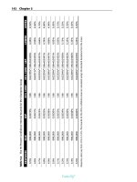
Figure 9.11 is an example of how the calculation takes place. In this example,
choosing a minimum support level of 10 percent would eliminate all the com-
binations with three items—and their associated rules—from consideration.
This is an example where pruning does not have an effect on the best rule since
the best rule has only two items. In the case of pizza, these toppings are all
fairly common, so are not pruned individually. If anchovies were included in
the analysis—and there are only 15 pizzas containing them out of the 2,000—
then a minimum support of 10 percent, or even 1 percent, would eliminate
anchovies during the first pass.
The best choice for minimum support depends on the data and the situa-
tion. It is also possible to vary the minimum support as the algorithm pro-
gresses. For instance, using different levels at different stages you can find
uncommon combinations of common items (by decreasing the support level
for successive steps) or relatively common combinations of uncommon items

(by increasing the support level).
The Problem of Big Data
A typical fast food restaurant offers several dozen items on its menu, say 100.
To use probabilities to generate association rules, counts have to be calculated
for each combination of items. The number of combinations of a given size
tends to grow exponentially. A combination with three items might be a small
fries, cheeseburger, and medium Diet Coke. On a menu with 100 items, how
many combinations are there with three different menu items? There are
161,700! This calculation is based on the binomial formula On the other hand,
a typical supermarket has at least 10,000 different items in stock, and more typ-
ically 20,000 or 30,000.
Figure 9.11 This example shows how to count up the frequencies on pizza sales for
market basket analysis.
Calculating the support, confidence, and lift quickly gets out of hand as the
number of items in the combinations grows. There are almost 50 million pos-
sible combinations of two items in the grocery store and over 100 billion com-
binations of three items. Although computers are getting more powerful and
A pizza restaurant has sold 2000 pizzas, of which:
100 are mushroom only, 150 are pepperoni, 200 are extra cheese
400 are mushroom and pepperoni, 300 are mushroom and extra cheese, 200 are pepperoni and extra cheese
100 are mushroom, pepperoni, and extra cheese.
550 have no extra toppings.
We need to calculate the probabilities for all possible combinations of items.
There are three rules with all three items:
Support = 5%
Confidence = 5% divided by 25% = 0.2
Lift = 20%(100/500) divided by 40%(800/2000) = 0.5
100 pizzas or 5%
100 + 400 + 300 + 100 = 900 pizzas or 45%
150 + 400 + 200 + 100 = 850 pizzas or 42.5%

200 + 300 + 200 + 100 = 800 pizzas or 40%
400 + 100 = 500 pizzas or 25%
300 + 100 = 400 pizzas or 20%
200 + 100 = 300 pizzas or 15%
Support = 5%
Confidence = 5% divided by 20% = 0.25
Lift = 25%(100/400) divided by 42.5%(850/2000) = 0.588
Support = 5%
Confidence = 5% divided by 15% = 0.333
Lift = 33.3%(100/300) divided by 45%(900/2000) = 0.74
Support = 25%
Confidence = 25% divided by 42.5% = 0.588
Lift = 55.6%(500/900) divided by 43.5%(200/850) = 1.31
The best rule has
only two items:
Just mushroom
Mushroom and pepperoni
Mushroom and extra cheese
The works
314 Chapter 9
470643 c09.qxd 3/8/04 11:15 AM Page 314
470643 c09.qxd 3/8/04 11:15 AM Page 315
Market Basket Analysis and Association Rules 315
cheaper, it is still very time-consuming to calculate the counts for this number
of combinations. Calculating the counts for five or more items is prohibitively
expensive. The use of product hierarchies reduces the number of items to a
manageable size.
The number of transactions is also very large. In the course of a year, a
decent-size chain of supermarkets will generate tens or hundreds of millions
of transactions. Each of these transactions consists of one or more items, often

several dozen at a time. So, determining if a particular combination of items is
present in a particular transaction may require a bit of effort—multiplied a
million-fold for all the transactions.
Extending the Ideas
The basic ideas of association rules can be applied to different areas, such as
comparing different stores and making some enhancements to the definition
of the rules. These are discussed in this section.
Using Association Rules to Compare Stores
Market basket analysis is commonly used to make comparisons between loca-
tions within a single chain. The rule about toilet bowl cleaner sales in hardware
stores is an example where sales at new stores are compared to sales at existing
stores. Different stores exhibit different selling patterns for many reasons:
regional trends, the effectiveness of management, dissimilar advertising, and
varying demographic patterns in the catchment area, for example. Air condi-
tioners and fans are often purchased during heat waves, but heat waves affect
only a limited region. Within smaller areas, demographics of the catchment
area can have a large impact; we would expect stores in wealthy areas to exhibit
different sales patterns from those in poorer neighborhoods. These are exam-
ples where market basket analysis can help to describe the differences and
serve as an example of using market basket analysis for directed data mining.
How can association rules be used to make these comparisons? The first
step is augmenting the transactions with virtual items that specify which
group, such as an existing location or a new location, that the transaction
comes from. Virtual items help describe the transaction, although the virtual
item is not a product or service. For instance, a sale at an existing hardware
store might include the following products:
■■ A hammer
■■ A box of nails
■■ Extra-fine sandpaper
470643 c09.qxd 3/8/04 11:15 AM Page 316

316 Chapter 9
TIP Adding virtual transactions in to the market basket data makes it possible
to find rules that include store characteristics and customer characteristics.
After augmenting the data to specify where it came from, the transaction
looks like:
a hammer,
a box of nails,
extra fine sandpaper,
“at existing hardware store.”
To compare sales at store openings versus existing stores, the process is:
1. Gather data for a specific period (such as 2 weeks) from store openings.
Augment each of the transactions in this data with a virtual item saying
that the transaction is from a store opening.
2. Gather about the same amount of data from existing stores. Here you
might use a sample across all existing stores, or you might take all the
data from stores in comparable locations. Augment the transactions in
this data with a virtual item saying that the transaction is from an exist-
ing store.
3. Apply market basket analysis to find association rules in each set.
4. Pay particular attention to association rules containing the virtual items.
Because association rules are undirected data mining, the rules act as start-
ing points for further hypothesis testing. Why does one pattern exist at exist-
ing stores and another at new stores? The rule about toilet bowl cleaners and
store openings, for instance, suggests looking more closely at toilet bowl
cleaner sales in existing stores at different times during the year.
Using this technique, market basket analysis can be used for many other
types of comparisons:
■■ Sales during promotions versus sales at other times
■■ Sales in various geographic areas, by county, standard statistical metro-
politan area (SSMA), direct marketing area (DMA), or country

■■ Urban versus suburban sales
■■ Seasonal differences in sales patterns
Adding virtual items to each basket of goods enables the standard associa-
tion rule techniques to make these comparisons.
470643 c09.qxd 3/8/04 11:15 AM Page 317
Market Basket Analysis and Association Rules 317
Dissociation Rules
A dissociation rule is similar to an association rule except that it can have the
connector “and not” in the condition in addition to “and.” A typical dissocia-
tion rule looks like:
if A and not B, then C.
Dissociation rules can be generated by a simple adaptation of the basic mar-
ket basket analysis algorithm. The adaptation is to introduce a new set of items
that are the inverses of each of the original items. Then, modify each transaction
so it includes an inverse item if, and only if, it does not contain the original item.
For example, Table 9.8 shows the transformation of a few transactions. The ¬
before the item denotes the inverse item.
There are three downsides to including these new items. First, the total
number of items used in the analysis doubles. Since the amount of computa-
tion grows exponentially with the number of items, doubling the number of
items seriously degrades performance. Second, the size of a typical transaction
grows because it now includes inverted items. The third issue is that the fre-
quency of the inverse items tends to be much larger than the frequency of the
original items. So, minimum support constraints tend to produce rules in
which all items are inverted, such as:
if NOT A and NOT B then NOT C.
These rules are less likely to be actionable.
Sometimes it is useful to invert only the most frequent items in the set used
for analysis. This is particularly valuable when the frequency of some of the
original items is close to 50 percent, so the frequencies of their inverses are also

close to 50 percent.
Table 9.8 Transformation of Transactions to Generate Dissociation Rules
CUSTOMER ITEMS CUSTOMER WITH INVERSE ITEMS
1 {A, B, C} 1 {A, B, C}
2 {A} 2 {A, ¬B, ¬C}
3 {A, C} 3 {A, ¬B, C}
4 {A} 4 {A, ¬B, ¬C}
5 {} 5 {¬A, ¬B, ¬C}
470643 c09.qxd 3/8/04 11:15 AM Page 318
318 Chapter 9
Sequential Analysis Using Association Rules
Association rules find things that happen at the same time—what items are
purchased at a given time. The next natural question concerns sequences of
events and what they mean. Examples of results in this area are:
■■ New homeowners purchase shower curtains before purchasing furniture.
■■ Customers who purchase new lawnmowers are very likely to purchase
a new garden hose in the following 6 weeks.
■■ When a customer goes into a bank branch and asks for an account rec-
onciliation, there is a good chance that he or she will close all his or her
accounts.
Time-series data usually requires some way of identifying the customer
over time. Anonymous transactions cannot reveal that new homeowners buy
shower curtains before they buy furniture. This requires tracking each cus-
tomer, as well as knowing which customers recently purchased a home. Since
larger purchases are often made with credit cards or debit cards, this is less of
a problem. For problems in other domains, such as investigating the effects of
medical treatments or customer behavior inside a bank, all transactions typi-
cally include identity information.
WARNING In order to consider time-series analyses on your customers,
there has to be some way of identifying customers. Without a way of tracking

individual customers, there is no way to analyze their behavior over time.
For the purposes of this section, a time series is an ordered sequence of items.
It differs from a transaction only in being ordered. In general, the time series
contains identifying information about the customer, since this information is
used to tie the different transactions together into a series. Although there are
many techniques for analyzing time series, such as ARIMA (a statistical tech-
nique) and neural networks, this section discusses only how to manipulate the
time-series data to apply the market basket analysis.
In order to use time series, the transaction data must have two additional
features:
■■ A timestamp or sequencing information to determine when transac-
tions occurred relative to each other
■■ Identifying information, such as account number, household ID, or cus-
tomer ID that identifies different transactions as belonging to the same
customer or household (sometimes called an economic marketing unit)
470643 c09.qxd 3/8/04 11:15 AM Page 319
Market Basket Analysis and Association Rules 319
Building sequential rules is similar to the process of building association
rules:
1. All items purchased by a customer are treated as a single order, and
each item retains the timestamp indicating when it was purchased.
2. The process is the same for finding groups of items that appear
together.
3. To develop the rules, only rules where the items on the left-hand side
were purchased before items on the right-hand side are considered.
The result is a set of association rules that can reveal sequential patterns.
Lessons Learned
Market basket data describes what customers purchase. Analyzing this data is
complex, and no single technique is powerful enough to provide all the
answers. The data itself typically describes the market basket at three different

levels. The order is the event of the purchase; the line-items are the items in the
purchase, and the customer connects orders together over time.
Many important questions about customer behavior can be answered by
looking at product sales over time. Which are the best selling items? Which
items that sold well last year are no longer selling well this year? Inventory
curves do not require transaction level data. Perhaps the most important
insight they provide is the effect of marketing interventions—did sales go up
or down after a particular event?
However, inventory curves are not sufficient for understanding relation-
ships among items in a single basket. One technique that is quite powerful is
association rules. This technique finds products that tend to sell together in
groups. Sometimes is the groups are sufficient for insight. Other times, the
groups are turned into explicit rules—when certain items are present then we
expect to find certain other items in the basket.
There are three measures of association rules. Support tells how often the
rule is found in the transaction data. Confidence says how often when the “if”
part is true that the “then” part is also true. And, lift tells how much better the
rule is at predicting the “then” part as compared to having no rule at all.
The rules so generated fall into three categories. Useful rules explain a rela-
tionship that was perhaps unexpected. Trivial rules explain relationships that
are known (or should be known) to exist. And inexplicable rules simply do not
make sense. Inexplicable rules often have weak support.
470643 c09.qxd 3/8/04 11:15 AM Page 320
320 Chapter 9
Market basket analysis and association rules provide ways to analyze item-
level detail, where the relationships between items are determined by the
baskets they fall into. In the next chapter, we’ll turn to link analysis, which
generalizes the ideas of “items” linked by “relationships,” using the back-
ground of an area of mathematics called graph theory.
470643 c10.qxd 3/8/04 11:16 AM Page 321

Link Analysis
10
CHAPTER
The international route maps of British Airways and Air France offer more
than just trip planning help. They also provide insights into the history and
politics of their respective homelands and of lost empires. A traveler bound
from New York to Mombasa changes planes at Heathrow; one bound for
Abidjan changes at Charles de Gaul. The international route maps show how
much information can be gained from knowing how things are connected.
Which Web sites link to which other ones? Who calls whom on the tele-
phone? Which physicians prescribe which drugs to which patients? These
relationships are all visible in data, and they all contain a wealth of informa-
tion that most data mining techniques are not able to take direct advantage of.
In our ever-more-connected world (where, it has been claimed, there are no
more than six degrees of separation between any two people on the planet),
understanding relationships and connections is critical. Link analysis is the
data mining technique that addresses this need.
Link analysis is based on a branch of mathematics called graph theory. This
chapter reviews the key notions of graphs, then shows how link analysis has
been applied to solve real problems. Link analysis is not applicable to all types
of data nor can it solve all types of problems. However, when it can be used, it
321
470643 c10.qxd 3/8/04 11:16 AM Page 322
322 Chapter 10
often yields very insightful and actionable results. Some areas where it has
yielded good results are:
■■ Identifying authoritative sources of information on the World Wide
Web by analyzing the links between its pages
■■ Analyzing telephone call patterns to identify particular market seg-
ments such as people working from home

■■ Understanding physician referral patterns; a referral is a relationship
between two physicians, once again, naturally susceptible to link analysis
Even where links are explicitly recorded, assembling them into a useful
graph can be a data-processing challenge. Links between Web pages are
encoded in the HTML of the pages themselves. Links between telephones
are recorded in call detail records. Neither of these data sources is useful for
link analysis without considerable preprocessing, however. In other cases, the
links are implicit and part of the data mining challenge is to recognize them.
The chapter begins with a brief introduction to graph theory and some of
the classic problems that it has been used to solve. It then moves on to appli-
cations in data mining such as search engine rankings and analysis of call
detail records.
Basic Graph Theory
Graphs are an abstraction developed specifically to represent relationships.
They have proven very useful in both mathematics and computer science for
developing algorithms that exploit these relationships. Fortunately, graphs are
quite intuitive, and there is a wealth of examples that illustrate how to take
advantage of them.
A graph consists of two distinct parts:
■■ Nodes (sometimes called vertices) are the things in the graph that have
relationships. These have names and often have additional useful
properties.
■■ Edges are pairs of nodes connected by a relationship. An edge is repre-
sented by the two nodes that it connects, so (A, B) or AB represents the
edge that connects A and B. An edge might also have a weight in a
weighted graph.
Figure 10.1 illustrates two graphs. The graph on the left has four nodes con-
nected by six edges and has the property that there is an edge between every
pair of nodes. Such a graph is said to be fully connected. It could be represent-
ing daily flights between Atlanta, New York, Cincinnati, and Salt Lake City on

an airline where these four cities serve as regional hubs. It could also represent
TEAMFLY

Team-Fly
®

470643 c10.qxd 3/8/04 11:16 AM Page 323
Link Analysis 323

four people, all of whom know each other, or four mutually related leads for a
criminal investigation. The graph on the right has one node in the center con-
nected to four other nodes. This could represent daily flights connecting
Atlanta to Birmingham, Greenville, Charlotte, and Savannah on an airline that
serves the Southeast from a hub in Atlanta, or a restaurant frequented by four
credit card customers. The graph itself captures the information about what is
connected to what. Without any labels, it can describe many different situa-
tions. This is the power of abstraction.
A few points of terminology about graphs. Because graphs are so useful for
visualizing relationships, it is nice when the nodes and edges can be drawn
with no intersecting edges. The graphs in Figure 10.2 have this property. They
are planar graphs, since they can be drawn on a sheet of paper (what mathe-
maticians call a plane) without having any edges intersect. Figure 10.2 shows
two graphs that cannot be drawn without having at least two edges cross.
There is, in fact, a theorem in graph theory that says that if a graph is nonpla-
nar, then lurking inside it is one of the two previously described graphs.
When a path exists between any two nodes in a graph, the graph is said to
be connected. For the rest of this chapter, we assume that all graphs are con-
nected, unless otherwise specified. A path, as its name implies, is an ordered
sequence of nodes connected by edges. Consider a graph where each node
represents a city, and the edges are flights between pairs of cities. On such a
graph, a node is a city and an edge is a flight segment—two cities that are con-
nected by a nonstop flight. A path is an itinerary of flight segments that go
from one city to another, such as from Greenville, South Carolina to Atlanta,
from Atlanta to Chicago, and from Chicago to Peoria.
A fully connected graph with
A graph with five nodes
four nodes and six edges. In
and four edges.
a fully connected graph, there

is an edge between every pair
of nodes.
Figure 10.1 Two examples of graphs.
470643 c10.qxd 3/8/04 11:16 AM Page 324
324 Chapter 10
Three nodes cannot connect
to three other nodes without
intersect.
two edges crossing over
each other.
A fully-connected graph
with five nodes must also
have edges that intersect.
Oops! These edges
Figure 10.2 Not all graphs can be drawn without having some edges cross over each other.
Figure 10.3 is an example of a weighted graph, one in which the edges have
weights associated with them. In this case, the nodes represent products pur-
chased by customers. The weights on the edges represent the support for the
association, the percentage of market baskets containing both products. Such
graphs provide an approach for solving problems in market basket analysis
and are also a useful means of visualizing market basket data. This product
association graph is an example of an undirected graph. The graph shows that
22.12 percent of market baskets at this health food grocery contain both yellow
peppers and bananas. By itself, this does not explain whether yellow pepper
sales drive banana sales or vice versa, or whether something else drives the
purchase of all yellow fruits and vegetables.
One very common problem in link analysis is finding the shortest path
between two nodes. Which is shortest, though, depends on the weights
assigned to the edges. Consider the graph of flights between cities. Does short-
est refer to distance? To the fewest number of flight segments? To the shortest

flight time? Or to the least expensive? All these questions are answered the
same way using graphs—the only difference is the weights on the edges.
The following two sections describe two classic problems in graph theory
that illustrate the power of graphs to represent and solve problems. Few data
mining problems are exactly like these two problems, but the problems give a
flavor of how the simple construction of graphs leads to some interesting solu-
tions. They are presented to familiarize the reader with graphs by providing
examples of key concepts in graph theory and to provide a stronger basis for
discussing link analysis.
470643 c10.qxd 3/8/04 11:16 AM Page 325
Link Analysis 325
Body Care
Organic Broccoli
Kitchen
Bananas
Red Leaf
Salad Mix
3
.2
5
8
.58
5.21
7.32
3.35
3.4
3
.
7
6.63

6.
2
8
Yellow Peppers
Red Peppers
Vine Tomatoes
Organic Peaches
Floral
3.68
Figure 10.3 This is an example of a weighted graph where the edge weights are the
number of transactions containing the items represented by the nodes at either end.
Seven Bridges of Königsberg
One of the earliest problems in graph theory originated with a simple chal-
lenge posed in the eighteenth century by the Swiss mathematician Leonhard
Euler. As shown in the simple map in Figure 10.4, Königsberg had two islands
in the Pregel River connected to each other and to the rest of the city by a total
of seven bridges. On either side of the river or on the islands, it is possible to
get to any of the bridges. Figure 10.4 shows one path through the town that
crosses over five bridges exactly once. Euler posed the question: Is it possible
to walk over all seven bridges exactly once, starting from anywhere in the city,
without getting wet or using a boat? As an historical note, the problem has sur-
vived longer than the name of the city. In the eighteenth century, Königsberg
was a prominent Prussian city on the Baltic Sea nestled between Lithuania and
Poland. Now, it is known as Kaliningrad, the westernmost Russian enclave,
separated from the rest of Russia by Lithuania and Belarus.
In order to solve this problem, Euler invented the notation of graphs. He rep-
resented the map of Königsberg as the simple graph with four vertices and seven
edges in Figure 10.5. Some pairs of nodes are connected by more than one edge,
indicating that there is more than one bridge between them. Finding a route that
traverses all the bridges in Königsberg exactly one time is equivalent to finding a

path in the graph that visits every edge exactly once. Such a path is called an
Eulerian path in honor of the mathematician who posed and solved this problem.
470643 c10.qxd 3/8/04 11:16 AM Page 326
326 Chapter 10
A
B
C
D
N
S
EW
Pregel River
Figure 10.4 The Pregel River in Königsberg has two islands connected by a total of seven
bridges.
A
C D
A
C
1
A
C
2
AD
BD
B
C
2
B
C
1

CD
B
Figure 10.5 This graph represents the layout of Königsberg. The edges are bridges and the
nodes are the riverbanks and islands.
470643 c10.qxd 3/8/04 11:16 AM Page 327
Link Analysis 327
Showing that an Eulerian path exists only when the degrees on all nodes are
about paths in the graph. Consider one path through the bridges:
A → C → B →C →D
AC
1
→ BC
1
→ BC
2
→ CD
four edges visiting it, and node B has two. Since the edges come in pairs, each
path contains all edges in the graph and visits all the nodes, such a path exists
only when all the nodes in the graph (minus the two end nodes) can serve as
of those nodes is even.
graph. By keeping track of the degrees of the nodes, it is possible to construct
such a path when there are at most two nodes whose degree is odd.
WHY DO THE DEGREES HAVE TO BE EVEN?
even (except at most two) rests on a simple observation. This observation is
The edges being used are:
The edges connecting the intermediate nodes in the path come in pairs. That
is, there is an outgoing edge for every incoming edge. For instance, node C has
intermediate node has an even number of edges in the path. Since an Eulerian
intermediate nodes for the path. This is another way of saying that the degree
Euler also showed that the opposite is true. When all the nodes in a graph

(save at most two) have an even degree, then an Eulerian path exists. This
proof is a bit more complicated, but the idea is rather simple. To construct an
Eulerian path, start at any node (even one with an odd degree) and move to
any other connected node which has an even degree. Remove the edge just
traversed from the graph and make it the first edge in the Eulerian path. Now,
the problem is to find an Eulerian path starting at the second node in the
Euler devised a solution based on the number of edges going into or out of
each node in the graph. The number of such edges is called the degree of a
node. For instance, in the graph representing the seven bridges of Königsberg,
the nodes representing the shores both have a degree of three—corresponding
to the fact that there are three bridges connecting each shore to the islands. The
other two nodes, representing the islands, have degrees of 5 and 3. Euler
showed that an Eulerian path exists only when the degrees of all the nodes in
a graph are even, except at most two (see technical aside). So, there is no way
to walk over the seven bridges of Königsberg without traversing a bridge
more than once, since there are four nodes whose degrees are odd.
Traveling Salesman Problem
A more recent problem in graph theory is the “Traveling Salesman Problem.”
In this problem, a salesman needs to visit customers in a set of cities. He plans
on flying to one of the cities, renting a car, visiting the customer there, then
driving to each of other cities to visit each of the rest of his customers. He
470643 c10.qxd 3/8/04 11:16 AM Page 328
328 Chapter 10
leaves the car in the last city and flies home. There are many possible routes
that the salesman can take. What route minimizes the total distance that he
travels while still allowing him to visit each city exactly one time?
The Traveling Salesman Problem is easily reformulated using graphs, since
graphs are a natural representation of cities connected by roads. In the graph
representing this problem, the nodes are cities and each edge has a weight cor-
responding to the distance between the two cities connected by the edge. The

Traveling Salesman Problem therefore is asking: “What is the shortest path
that visits all the nodes in a graph exactly one time?” Notice that this problem
is different from the Seven Bridges of Königsberg. We are not interested in sim-
ply finding a path that visits all nodes exactly once, but of all possible paths we
want the shortest one. Notice that all Eulerian paths have exactly the same
length, since they contain exactly the same edges. Asking for the shortest
Eulerian path does not make sense.
Solving the Traveling Salesman Problem for three or four cities is not diffi-
cult. The most complicated graph with four nodes is a completely connected
graph where every node in the graph is connected to every other node. In this
graph, 24 different paths visit each node exactly once. To count the number of
paths, start at any of nodes (there are four possibilities), then go to any of the
other three remaining ones, then to any of the other two, and finally to the last
node (4
*
3
*
2
*
1 = 4! = 24). A completely connected graph with n nodes has n!
(n factorial) distinct paths that contain all nodes. Each path has a slightly dif-
ferent collection of edges, so their lengths are usually different. Since listing
the 24 possible paths is not that hard, finding the shortest path is not particu-
larly difficult for this simple case.
The problem of finding the shortest path connecting nodes was first investi-
gated by the Irish mathematician Sir William Rowan Hamilton. His study of
minimizing energy in physical systems led him to investigate minimizing
energy in certain discrete systems that he represented as graphs. In honor of
him, a path that visits all nodes in a graph exactly once is called a Hamiltonian
path.

The Traveling Salesman Problem is difficult to solve. Any solution must con-
sider all of the possible paths through the graph in order to determine which
one is the shortest. The number of paths in a completely connected graph grows
very fast—as a factorial. What is true for completely connected graphs is true
for graphs in general: The number of possible paths visiting all the nodes grows
like an exponential function of the number of nodes (although there are a few
simple graphs where this is not true). So, as the number of cities increases, the
effort required to find the shortest path grows exponentially. Adding just one
more city (with associated roads) can result in a solution that takes twice as
long—or more—to find.
470643 c10.qxd 3/8/04 11:16 AM Page 329
Link Analysis 329
This lack of scalability is so important that mathematicians have given it a
name: NP—where NP means that all known algorithms used to solve the
problem scale exponentially—not like a polynomial. These problems are con-
sidered difficult. In fact, the Traveling Salesman Problem is so difficult that it is
used for evaluating parallel computers and exotic computing methods—such
as using DNA or the mysteries of quantum physics as the basis of computers
instead of the more familiar computer chips made of silicon.
All of this graph theory aside, there are pretty good heuristic algorithms for
computers that provide reasonable solutions to the Traveling Salesman
Problem. The resulting paths are relatively short paths, although they are not
guaranteed to be as short as the shortest possible one. This is a useful fact if
you have a similar problem. One common algorithm is the greedy algorithm:
start the path with the shortest edge in the graph, then lengthen the path
with the shortest edge available at either end that visits a new node. The result-
ing path is generally pretty short, although not necessarily the shortest (see
Figure 10.6).
TIP Often it is better to use an algorithm that yields good, but not perfect
results, instead of trying to analyze the difficulty of arriving at the ideal solution

or giving up because there is no guarantee of finding an optimal solution. As
Voltaire remarked, “Le mieux est l’ennemi du bien.” (The best is the enemy of
the good.)
A
B C D 9
18
11
2
1
12
2 E
Figure 10.6 In this graph, the shortest path (ABCDE) has a length of 24, but the greedy
algorithm finds a much longer path (CDBEA).
470643 c10.qxd 3/8/04 11:16 AM Page 330
330 Chapter 10
Directed Graphs
The graphs discussed so far are undirected. In undirected graphs, the edges
are like expressways between nodes: they go in both directions. In a directed
graph, the edges are like one-way roads. An edge going from A to B is distinct
from an edge going from B to A. A directed edge from A to B is an outgoing edge
of A and an incoming edge of B.
Directed graphs are a powerful way of representing data:
■■ Flight segments that connect a set of cities
■■ Hyperlinks between Web pages
■■ Telephone calling patterns
■■ State transition diagrams
Two types of nodes are of particular interest in directed graphs. All the
edges connected to a source node are outgoing edges. Since there are no incom-
ing edges, no path exists from any other node in the graph to any of the source
nodes. When all the edges on a node are incoming edges, the node is called a

sink node. The existence of source nodes and sink nodes is an important differ-
ence between directed graphs and their undirected cousins.
An important property of directed graphs is whether the graph contains any
paths that start and end at the same vertex. Such a path is called a cycle, imply-
ing that the path could repeat itself endlessly: ABCABCABC and so on. If a
directed graph contains at least one cycle, it is called cyclic. Cycles in a graph of
flight segments, for instance, might be the path of a single airplane. In a call
graph, members of a cycle call each other—these are good candidates for a
“friends and family–style” promotion, where the whole group gets a discount,
or for marketing conference call services.
Detecting Cycles in a Graph
There is a simple algorithm to detect whether a directed graph has any cycles.
This algorithm starts with the observation that if a directed graph has no sink
vertices, and it has at least one edge, then any path can be extended arbitrarily.
Without any sink vertices, the terminating node of a path is always connected
to another node, so the path can be extended by appending that node. Simi-
larly, if the graph has no source nodes, then we can always prepend a node to
the beginning of the path. Once the path contains more nodes than there are
nodes in the graph, we know that the path must visit at least one node twice.
Call this node X. The portion of the path between the first X and the second X
in the path is a cycle, so the graph is cyclic.
Now consider the case when a graph has one or more source nodes and one
or more sink nodes. It is pretty obvious that source nodes and sink nodes
470643 c10.qxd 3/8/04 11:16 AM Page 331
Link Analysis 331
cannot be part of a cycle. Removing the source and sink nodes from the graph,
along with all their edges, does not affect whether the graph is cyclic. If the
resulting graph has no sink nodes or no source nodes, then it contains a cycle,
as just shown. The process of removing sink nodes, source nodes, and their
edges is repeated until one of the following occurs:

■■ No more edges or no more nodes are left. In this case, the graph has no
cycles.
■■ Some edges remain but there are no source or sink nodes. In this case,
the graph is cyclic.
If no cycles exist, then the graph is called an acyclic graph. These graphs are
useful for describing dependencies or one-way relationships between things.
For instance, different products often belong to nested hierarchies that can be
represented by acyclic graphs. The decision trees described in Chapter 6 are
another example.
In an acyclic graph, any two nodes have a well-defined precedence relation-
ship with each other. If node A precedes node B in some path that contains both
A and B, then A will precede B in all paths containing both A and B (otherwise
there would be a cycle). In this case, we say that A is a predecessor of B and that
B is a successor of A. If no paths contain both A and B, then A and B are disjoint.
This strict ordering can be an important property of the nodes and is sometimes
useful for data mining purposes.
A Familiar Application of Link Analysis
Most readers of this book have probably used the Google search engine. Its
phenomenal popularity stems from its ability to help people find reasonably
good material on pretty much any subject. This feat is accomplished through
link analysis.
The World Wide Web is a huge directed graph. The nodes are Web pages and
the edges are the hyperlinks between them. Special programs called spiders or
web crawlers are continually traversing these links to update maps of the huge
directed graph that is the web. Some of these spiders simply index the content
of Web pages for use by purely text-based search engines. Others record the
Web’s global structure as a directed graph that can be used for analysis.
Once upon a time, search engines analyzed only the nodes of this graph.
Text from a query was compared with text from the Web pages using tech-
niques similar to those described in Chapter 8. Google’s approach (which has

now been adopted by other search engines) is to make use of the information
encoded in the edges of the graph as well as the information found in the nodes.
470643 c10.qxd 3/8/04 11:16 AM Page 332
332 Chapter 10
The Kleinberg Algorithm
Some Web sites or magazine articles are more interesting than others even if
they are devoted to the same topic. This simple idea is easy to grasp but hard
to explain to a computer. So when a search is performed on a topic that many
people write about, it is hard to find the most interesting or authoritative
documents in the huge collection that satisfies the search criteria.
Professor Jon Kleinberg of Cornell University came up with one widely
adopted technique for addressing this problem. His approach takes advantage
of the insight that in creating a link from one site to another, a human being is
making a judgment about the value of the site being linked to. Each link to
another site is effectively a recommendation of that site. Cumulatively, the
independent judgments of many Web site designers who all decide to provide
links to the same target are conferring authority on that target. Furthermore,
the reliability of the sites making the link can be judged according to the
authoritativeness of the sites they link to. The recommendations of a site with
many other good recommendations can be given more weight in determining
the authority of another.
In Kleinberg’s terminology, a page that links to many authorities is a hub; a
page that is linked to by many hubs is an authority. These ideas are illustrated
in Figure 10.7 The two concepts can be used together to tell the difference
between authority and mere popularity. At first glance, it might seem that a
good method for finding authoritative Web sites would be to rank them by the
number of unrelated sites linking to them. The problem with this technique is
that any time the topic is mentioned, even in passing, by a popular site (one
with many inbound links), it will be ranked higher than a site that is much
more authoritative on the particular subject though less popular in general.

The solution is to rank pages, not by the total number of links pointing
to them, but by the number of subject-related hubs that point to them.
Google.com uses a modified and enhanced version of the basic Kleinberg
algorithm described here.
A search based on link analysis begins with an ordinary text-based search.
This initial search provides a pool of pages (often a couple hundred) with
which to start the process. It is quite likely that the set of documents returned
by such a search does not include the documents that a human reader would
judge to be the most authoritative sources on the topic. That is because the
most authoritative sources on a topic are not necessarily the ones that use the
words in the search string most frequently. Kleinberg uses the example of
a search on the keyword “Harvard.” Most people would agree that www.
harvard.edu is one of the most authoritative sites on this topic, but in a purely
content-based analysis, it does not stand out among the more than a million
Web pages containing the word “Harvard” so it is quite likely that a text-based
search will not return the university’s own Web site among its top results. It is
very likely, however, that at least a few of the documents returned will contain
TEAMFLY

Team-Fly
®

470643 c10.qxd 3/8/04 11:16 AM Page 333
Link Analysis 333
a link to Harvard’s home page or, failing that, that some page that points to
one of the pages in the pool of pages will also point to www.harvard.edu.
An essential feature of Kleinberg’s algorithm is that it does not simply take
the pages returned by the initial text-based search and attempt to rank them; it
uses them to construct the much larger pool of documents that point to or are
pointed to by any of the documents in the root set. This larger pool contains
much more global structure—structure that can be mined to determine which
documents are considered to be most authoritative by the wide community of
people who created the documents in the pool.
The Details: Finding Hubs and Authorities
Kleinberg’s algorithm for identifying authoritative sources has three phases:
1. Creating the root set
2. Identifying the candidates
3. Ranking hubs and authorities

In the first phase, a root set of pages is formed using a text-based search
engine to find pages containing the search string. In the second phase, this root
set is expanded to include documents that point to or are pointed to by docu-
ments in the root set. This expanded set contains the candidates. In the third
phase, which is iterative, the candidates are ranked according to their strength
as hubs (documents that have links to many authoritative documents) and
authorities (pages that have links from many authoritative hubs).
Creating the Root Set
The root set of documents is generated using a content-based search. As a first
step, stop words (common words such as “a,” “an,” “the,” and so on) are
removed from the original search string supplied. Then, depending on the par-
ticular content-based search strategy employed, the remaining search terms
may undergo stemming. Stemming reduces words to their root form by remov-
ing plural forms and other endings due to verb conjugation, noun declension,
and so on. Then, the Web index is searched for documents containing the
terms in the search string. There are many variations on the details of how
matches are evaluated, which is one reason why performing the same search
on two text-based search engines yields different results. In any case, some
combination of the number of matching terms, the rarity of the terms matched,
and the number of times the search terms are mentioned in a document is used
to give the indexed documents a score that determines their rank in relation to
the query. The top n documents are used to establish the root set. A typical
value for n is 200.
470643 c10.qxd 3/8/04 11:16 AM Page 334
334 Chapter 10
Identifying the Candidates
In the second phase, the root set is expanded to create the set of candidates. The
candidate set includes all pages that any page in the root set links to along with
a subset of the pages that link to any page in the root set. Locating pages that
link to a particular target page is simple if the global structure of the Web is

available as a directed graph. The same task can also be accomplished with an
index-based text search using the URL of the target page as the search string.
The reason for using only a subset of the pages that link to each page in the
root set is to guard against the possibility of an extremely popular site in the
root set bringing in an unmanageable number of pages. There is also a param-
eter d that limits the number of pages that may be brought into the candidate
set by any single member of the root set.
If more than d documents link to a particular document in the root set, then
an arbitrary subset of d documents is brought into the candidate set. A typical
value for d is 50. The candidate set typically ends up containing 1,000 to 5,000
documents.
This basic algorithm can be refined in various ways. One possible refine-
ment, for instance, is to filter out any links from within the same domain,
many of which are likely to be purely navigational. Another refinement is to
allow a document in the root set to bring in at most m pages from the same site.
This is to avoid being fooled by “collusion” between all the pages of a site to,
for example, advertise the site of the Web site designer with a “this site
designed by” link on every page.
Ranking Hubs and Authorities
The final phase is to divide the candidate pages into hubs and authorities and
rank them according to their strength in those roles. This process also has the
effect of grouping together pages that refer to the same meaning of a search
term with multiple meanings—for instance, Madonna the rock star versus the
Madonna and Child in art history or Jaguar the car versus jaguar the big cat. It
also differentiates between authorities on the topic of interest and sites that are
simply popular in general. Authoritative pages on the correct topic are not
only linked to by many pages, they tend to be linked to by the same pages. It is
these hub pages that tie together the authorities and distinguish them from
unrelated but popular pages. Figure 10.7 illustrates the difference between
hubs, authorities, and unrelated popular pages.

Hubs and authorities have a mutually reinforcing relationship. A strong hub
is one that links to many strong authorities; a strong authority is one that is
linked to by many strong hubs. The algorithm therefore proceeds iteratively,
first adjusting the strength rating of the authorities based on the strengths of
the hubs that link to them and then adjusting the strengths of the hubs based
on the strength of the authorities to which they link.
470643 c10.qxd 3/8/04 11:16 AM Page 335
Link Analysis 335
Hubs Authorities Popular Site
Figure 10.7 Google uses link analysis to distinguish hubs, authorities, and popular pages.
For each page, there is a value A that measures its strength as an authority
and a value H that measures its strength as a hub. Both these values are ini-
tialized to 1 for all pages. Then, the A value for each page is updated by adding
up the H values of all the pages that link to them. The A values for each page
are then normalized so that the sum of their squares is equal to 1. Then the H
values are updated in a similar manner. The H value for each page is set to the
sum of the A values of the pages it links to, and the new H values are normal-
ized so that the sum of their squares is equal to 1. This process is repeated until
an equilibrium set of A and H values is reached. The pages that end up with
the highest H values are the strongest hubs; those with the strongest A values
are the strongest authorities.
The authorities returned by this application of link analysis tend to be
strong examples of one particular possible meaning of the search string. A
search on a contentious topic such as “gay marriage” or “Taiwan indepen-
dence” yields strong authorities on both sides because the global structure of
the Web includes tightly connected subgraphs representing documents main-
tained by like-minded authors.
470643 c10.qxd 3/8/04 11:16 AM Page 336
336 Chapter 10
Hubs and Authorities in Practice

The strongest case for the advantage of adding link analysis to text-based search-
ing comes from the market place. Google, a search engine developed at Stanford
by Sergey Brin and Lawence Page using an approach very similar to Klein-
berg’s, was the first of the major search engines to make use of link analysis to
find hubs and authorities. It quickly surpassed long-entrenched search services
such as AltaVista and Yahoo! The reason was qualitatively better searches.
The authors noticed that something was special about Google back in April
of 2001 when we studied the web logs from our company’s site, www
.data-miners.com. At that time, industry surveys gave Google and AltaVista
approximately equal 10 percent shares of the market for web searches, and yet
Google accounted for 30 percent of the referrals to our site while AltaVista
accounted for only 3 percent. This is apparently because Google was better
able to recognize our site as an authority for data mining consulting because it
was less confused by the large number of sites that use the phrase “data min-
ing” even though they actually have little to do with the topic.
Case Study: Who Is Using Fax Machines from Home?
Graphs appear in data from other industries as well. Mobile, local, and long-
distance telephone service providers have records of every telephone call that
their customers make and receive. This data contains a wealth of information
about the behavior of their customers: when they place calls, who calls them,
whether they benefit from their calling plan, to name a few. As this case study
shows, link analysis can be used to analyze the records of local telephone calls
to identify which residential customers have a high probability of having fax
machines in their home.
Why Finding Fax Machines Is Useful
What is the use of knowing who owns a fax machine? How can a telephone
provider act on this information? In this case, the provider had developed a
package of services for residential work-at-home customers. Targeting such
customers for marketing purposes was a revolutionary concept at the com-
pany. In the tightly regulated local phone market of not so long ago, local ser-

vice providers lost revenue from work-at-home customers, because these
customers could have been paying higher business rates instead of lower resi-
dential rates. Far from targeting such customers for marketing campaigns,
the local telephone providers would deny such customers residential rates—
punishing them for behaving like a small business. For this company, develop-
ing and selling work-at-home packages represented a new foray into customer
service. One question remained. Which customers should be targeted for the
new package?