Business process improvement_5 doc
Bạn đang xem bản rút gọn của tài liệu. Xem và tải ngay bản đầy đủ của tài liệu tại đây (1.92 MB, 29 trang )
Comparison
of the 3
central
composite
designs
The diagrams in Figure 3.21 illustrate the three types of central
composite designs for two factors. Note that the CCC explores the
largest process space and the CCI explores the smallest process space.
Both the CCC and CCI are rotatable designs, but the CCF is not. In the
CCC design, the design points describe a circle circumscribed about
the factorial square. For three factors, the CCC design points describe
a sphere around the factorial cube.
Determining
in Central Composite Designs
The value of
is chosen to
maintain
rotatability
To maintain rotatability, the value of
depends on the number of
experimental runs in the factorial portion of the central composite
design:
If the factorial is a full factorial, then
However, the factorial portion can also be a fractional factorial design
of resolution V.
Table 3.23 illustrates some typical values of as a function of the
number of factors.
Values of
depending on
the number of
factors in the
factorial part
of the design
TABLE 3.23 Determining
for Rotatability
Number of
Factors
Factorial
Portion
Scaled Value for
Relative to ±1
2
2
2
2
2/4
= 1.414
3
2
3
2
3/4
= 1.682
4
2
4
2
4/4
= 2.000
5
2
5-1
2
4/4
= 2.000
5
2
5
2
5/4
= 2.378
6
2
6-1
2
5/4
= 2.378
6
2
6
2
6/4
= 2.828
5.3.3.6.1. Central Composite Designs (CCD)
(4 of 5) [5/1/2006 10:30:40 AM]
Orthogonal
blocking
The value of also depends on whether or not the design is
orthogonally blocked. That is, the question is whether or not the
design is divided into blocks such that the block effects do not affect
the estimates of the coefficients in the 2nd order model.
Example of
both
rotatability
and
orthogonal
blocking for
two factors
Under some circumstances, the value of
allows simultaneous
rotatability and orthogonality. One such example for k = 2 is shown
below:
BLOCK X1 X2
1 -1 -1
1 1 -1
1 -1 1
1 1 1
1 0 0
1 0 0
2 -1.414 0
2 1.414 0
2 0 -1.414
2 0 1.414
2 0 0
2 0 0
Additional
central
composite
designs
Examples of other central composite designs will be given after
Box-Behnken designs are described.
5.3.3.6.1. Central Composite Designs (CCD)
(5 of 5) [5/1/2006 10:30:40 AM]
5. Process Improvement
5.3. Choosing an experimental design
5.3.3. How do you select an experimental design?
5.3.3.6. Response surface designs
5.3.3.6.2.Box-Behnken designs
An alternate
choice for
fitting
quadratic
models that
requires 3
levels of
each factor
and is
rotatable (or
"nearly"
rotatable)
The Box-Behnken design is an independent quadratic design in that it
does not contain an embedded factorial or fractional factorial design. In
this design the treatment combinations are at the midpoints of edges of
the process space and at the center. These designs are rotatable (or near
rotatable) and require 3 levels of each factor. The designs have limited
capability for orthogonal blocking compared to the central composite
designs.
Figure 3.22 illustrates a Box-Behnken design for three factors.
Box-Behnken
design for 3
factors
FIGURE 3.22 A Box-Behnken Design for Three Factors
5.3.3.6.2. Box-Behnken designs
(1 of 2) [5/1/2006 10:30:40 AM]
Geometry of
the design
The geometry of this design suggests a sphere within the process space
such that the surface of the sphere protrudes through each face with the
surface of the sphere tangential to the midpoint of each edge of the
space.
Examples of Box-Behnken designs are given on the next page.
5.3.3.6.2. Box-Behnken designs
(2 of 2) [5/1/2006 10:30:40 AM]
5. Process Improvement
5.3. Choosing an experimental design
5.3.3. How do you select an experimental design?
5.3.3.6. Response surface designs
5.3.3.6.3.Comparisons of response surface
designs
Choosing a Response Surface Design
Various
CCD designs
and
Box-Behnken
designs are
compared
and their
properties
discussed
Table 3.24 contrasts the structures of four common quadratic designs one might
use when investigating three factors. The table combines CCC and CCI designs
because they are structurally identical.
For three factors, the Box-Behnken design offers some advantage in requiring a
fewer number of runs. For 4 or more factors, this advantage disappears.
Structural
comparisons
of CCC
(CCI), CCF,
and
Box-Behnken
designs for
three factors
TABLE 3.24 Structural Comparisons of CCC (CCI), CCF, and
Box-Behnken Designs for Three Factors
CCC (CCI) CCF Box-Behnken
Rep X1 X2 X3 Rep X1 X2 X3 Rep X1 X2 X3
1 -1 -1 -1 1 -1 -1 -1 1 -1 -1 0
1 +1 -1 -1 1 +1 -1 -1 1 +1 -1 0
1 -1 +1 -1 1 -1 +1 -1 1 -1 +1 0
1 +1 +1 -1 1 +1 +1 -1 1 +1 +1 0
1 -1 -1 +1 1 -1 -1 +1 1 -1 0 -1
1 +1 -1 +1 1 +1 -1 +1 1 +1 0 -1
1 -1 +1 +1 1 -1 +1 +1 1 -1 0 +1
1 +1 +1 +1 1 +1 +1 +1 1 +1 0 +1
1 -1.682 0 0 1 -1 0 0 1 0 -1 -1
1 1.682 0 0 1 +1 0 0 1 0 +1 -1
1 0 -1.682 0 1 0 -1 0 1 0 -1 +1
1 0 1.682 0 1 0 +1 0 1 0 +1 +1
5.3.3.6.3. Comparisons of response surface designs
(1 of 5) [5/1/2006 10:30:41 AM]
1 0 0 -1.682 1 0 0 -1 3 0 0 0
1 0 0 1.682 1 0 0 +1
6 0 0 0 6 0 0 0
Total Runs = 20 Total Runs = 20 Total Runs = 15
Factor
settings for
CCC and
CCI three
factor
designs
Table 3.25 illustrates the factor settings required for a central composite
circumscribed (CCC) design and for a central composite inscribed (CCI) design
(standard order), assuming three factors, each with low and high settings of 10
and 20, respectively. Because the CCC design generates new extremes for all
factors, the investigator must inspect any worksheet generated for such a design
to make certain that the factor settings called for are reasonable.
In Table 3.25, treatments 1 to 8 in each case are the factorial points in the design;
treatments 9 to 14 are the star points; and 15 to 20 are the system-recommended
center points. Notice in the CCC design how the low and high values of each
factor have been extended to create the star points. In the CCI design, the
specified low and high values become the star points, and the system computes
appropriate settings for the factorial part of the design inside those boundaries.
TABLE 3.25 Factor Settings for CCC and CCI Designs for Three
Factors
Central Composite
Circumscribed CCC
Central Composite
Inscribed CCI
Sequence
Number
X1 X2 X3
Sequence
Number
X1 X2 X3
1 10 10 10 1 12 12 12
2 20 10 10 2 18 12 12
3 10 20 10 3 12 18 12
4 20 20 10 4 18 18 12
5 10 10 20 5 12 12 18
6 20 10 20 6 18 12 18
7 10 20 20 7 12 12 18
8 20 20 20 8 18 18 18
9 6.6 15 15 * 9 10 15 15
10 23.4 15 15 * 10 20 15 15
11 15 6.6 15 * 11 15 10 15
12 15 23.4 15 * 12 15 20 15
13 15 15 6.6 * 13 15 15 10
14 15 15 23.4 * 14 15 15 20
15 15 15 15 15 15 15 15
16 15 15 15 16 15 15 15
17 15 15 15 17 15 15 15
5.3.3.6.3. Comparisons of response surface designs
(2 of 5) [5/1/2006 10:30:41 AM]
18 15 15 15 18 15 15 15
19 15 15 15 19 15 15 15
20 15 15 15 20 15 15 15
* are star points
Factor
settings for
CCF and
Box-Behnken
three factor
designs
Table 3.26 illustrates the factor settings for the corresponding central composite
face-centered (CCF) and Box-Behnken designs. Note that each of these designs
provides three levels for each factor and that the Box-Behnken design requires
fewer runs in the three-factor case.
TABLE 3.26 Factor Settings for CCF and Box-Behnken Designs for
Three Factors
Central Composite
Face-Centered CCC
Box-Behnken
Sequence
Number
X1 X2 X3
Sequence
Number
X1 X2 X3
1 10 10 10 1 10 10 10
2 20 10 10 2 20 10 15
3 10 20 10 3 10 20 15
4 20 20 10 4 20 20 15
5 10 10 20 5 10 15 10
6 20 10 20 6 20 15 10
7 10 20 20 7 10 15 20
8 20 20 20 8 20 15 20
9 10 15 15 * 9 15 10 10
10 20 15 15 * 10 15 20 10
11 15 10 15 * 11 15 10 20
12 15 20 15 * 12 15 20 20
13 15 15 10 * 13 15 15 15
14 15 15 20 * 14 15 15 15
15 15 15 15 15 15 15 15
16 15 15 15
17 15 15 15
18 15 15 15
19 15 15 15
20 15 15 15
* are star points for the CCC
5.3.3.6.3. Comparisons of response surface designs
(3 of 5) [5/1/2006 10:30:41 AM]
Properties of
classical
response
surface
designs
Table 3.27 summarizes properties of the classical quadratic designs. Use this table
for broad guidelines when attempting to choose from among available designs.
TABLE 3.27 Summary of Properties of Classical Response Surface Designs
Design Type Comment
CCC
CCC designs provide high quality predictions over the entire
design space, but require factor settings outside the range of the
factors in the factorial part. Note: When the possibility of running
a CCC design is recognized before starting a factorial experiment,
factor spacings can be reduced to ensure that ±
for each coded
factor corresponds to feasible (reasonable) levels.
Requires 5 levels for each factor.
CCI
CCI designs use only points within the factor ranges originally
specified, but do not provide the same high quality prediction
over the entire space compared to the CCC.
Requires 5 levels of each factor.
CCF
CCF designs provide relatively high quality predictions over the
entire design space and do not require using points outside the
original factor range. However, they give poor precision for
estimating pure quadratic coefficients.
Requires 3 levels for each factor.
Box-Behnken
These designs require fewer treatment combinations than a
central composite design in cases involving 3 or 4 factors.
The Box-Behnken design is rotatable (or nearly so) but it contains
regions of poor prediction quality like the CCI. Its "missing
corners" may be useful when the experimenter should avoid
combined factor extremes. This property prevents a potential loss
of data in those cases.
Requires 3 levels for each factor.
5.3.3.6.3. Comparisons of response surface designs
(4 of 5) [5/1/2006 10:30:41 AM]
Number of
runs
required by
central
composite
and
Box-Behnken
designs
Table 3.28 compares the number of runs required for a given number of factors
for various Central Composite and Box-Behnken designs.
TABLE 3.28 Number of Runs Required by Central Composite and
Box-Behnken Designs
Number of Factors Central Composite Box-Behnken
2 13 (5 center points) -
3 20 (6 centerpoint runs) 15
4 30 (6 centerpoint runs) 27
5 33 (fractional factorial) or 52 (full factorial) 46
6 54 (fractional factorial) or 91 (full factorial) 54
Desirable Features for Response Surface Designs
A summary
of desirable
properties
for response
surface
designs
G. E. P. Box and N. R. Draper in "Empirical Model Building and Response
Surfaces," John Wiley and Sons, New York, 1987, page 477, identify desirable
properties for a response surface design:
Satisfactory distribution of information across the experimental region.
- rotatability
●
Fitted values are as close as possible to observed values.
- minimize residuals or error of prediction
●
Good lack of fit detection.●
Internal estimate of error.●
Constant variance check.●
Transformations can be estimated.●
Suitability for blocking.●
Sequential construction of higher order designs from simpler designs●
Minimum number of treatment combinations.●
Good graphical analysis through simple data patterns.●
Good behavior when errors in settings of input variables occur.●
5.3.3.6.3. Comparisons of response surface designs
(5 of 5) [5/1/2006 10:30:41 AM]
5. Process Improvement
5.3. Choosing an experimental design
5.3.3. How do you select an experimental design?
5.3.3.6. Response surface designs
5.3.3.6.4.Blocking a response surface design
How can we block a response surface design?
When
augmenting
a resolution
V design to
a CCC
design by
adding star
points, it
may be
desirable to
block the
design
If an investigator has run either a 2
k
full factorial or a 2
k-p
fractional factorial
design of at least resolution V, augmentation of that design to a central
composite design (either CCC of CCF) is easily accomplished by adding an
additional set (block) of star and centerpoint runs. If the factorial experiment
indicated (via the t test) curvature, this composite augmentation is the best
follow-up option (follow-up options for other situations will be discussed later).
An
orthogonal
blocked
response
surface
design has
advantages
An important point to take into account when choosing a response surface
design is the possibility of running the design in blocks. Blocked designs are
better designs if the design allows the estimation of individual and interaction
factor effects independently of the block effects. This condition is called
orthogonal blocking. Blocks are assumed to have no impact on the nature and
shape of the response surface.
CCF
designs
cannot be
orthogonally
blocked
The CCF design does not allow orthogonal blocking and the Box-Behnken
designs offer blocking only in limited circumstances, whereas the CCC does
permit orthogonal blocking.
5.3.3.6.4. Blocking a response surface design
(1 of 5) [5/1/2006 10:30:42 AM]
Axial and
factorial
blocks
In general, when two blocks are required there should be an axial block and a
factorial block. For three blocks, the factorial block is divided into two blocks
and the axial block is not split. The blocking of the factorial design points
should result in orthogonality between blocks and individual factors and
between blocks and the two factor interactions.
The following Central Composite design in two factors is broken into two
blocks.
Table of
CCD design
with 2
factors and
2 blocks
TABLE 3.29 CCD: 2 Factors, 2 Blocks
Pattern Block X1 X2 Comment
1 -1 -1 Full Factorial
-+ 1 -1 +1 Full Factorial
+- 1 +1 -1 Full Factorial
++ 1 +1 +1 Full Factorial
00 1 0 0 Center-Full Factorial
00 1 0 0 Center-Full Factorial
00 1 0 0 Center-Full Factorial
-0 2 -1.414214 0 Axial
+0 2 +1.414214 0 Axial
0- 2 0 -1.414214 Axial
0+ 2 0 +1.414214 Axial
00 2 0 0 Center-Axial
00 2 0 0 Center-Axial
00 2 0 0 Center-Axial
Note that the first block includes the full factorial points and three centerpoint
replicates. The second block includes the axial points and another three
centerpoint replicates. Naturally these two blocks should be run as two separate
random sequences.
Table of
CCD design
with 3
factors and
3 blocks
The following three examples show blocking structure for various designs.
TABLE 3.30 CCD: 3 Factors 3 Blocks, Sorted by Block
Pattern Block X1 X2 X3 Comment
1 -1 -1 -1 Full Factorial
-++ 1 -1 +1 +1 Full Factorial
+-+ 1 +1 -1 +1 Full Factorial
++- 1 +1 +1 -1 Full Factorial
000 1 0 0 0 Center-Full Factorial
000 1 0 0 0 Center-Full Factorial
+ 2 -1 -1 +1 Full Factorial
5.3.3.6.4. Blocking a response surface design
(2 of 5) [5/1/2006 10:30:42 AM]
-+- 2 -1 +1 -1 Full Factorial
+ 2 +1 -1 -1 Full Factorial
+++ 2 +1 +1 +1 Full Factorial
000 2 0 0 0 Center-Full Factorial
000 2 0 0 0 Center-Full Factorial
-00 3 -1.63299 0 0 Axial
+00 3 +1.63299 0 0 Axial
0-0 3 0 -1.63299 0 Axial
0+0 3 0 +1.63299 0 Axial
00- 3 0 0 -1.63299 Axial
00+ 3 0 0 +1.63299 Axial
000 3 0 0 0 Axial
000 3 0 0 0 Axial
Table of
CCD design
with 4
factors and
3 blocks
TABLE 3.31 CCD: 4 Factors, 3 Blocks
Pattern Block X1 X2 X3 X4 Comment
+ 1 -1 -1 -1 +1 Full Factorial
+- 1 -1 -1 +1 -1 Full Factorial
-+ 1 -1 +1 -1 -1 Full Factorial
-+++ 1 -1 +1 +1 +1 Full Factorial
+ 1 +1 -1 -1 -1 Full Factorial
+-++ 1 +1 -1 +1 +1 Full Factorial
++-+ 1 +1 +1 -1 +1 Full Factorial
+++- 1 +1 +1 +1 -1 Full Factorial
0000 1 0 0 0 0 Center-Full Factorial
0000 1 0 0 0 0 Center-Full Factorial
2 -1 -1 -1 -1 Full Factorial
++ 2 -1 -1 +1 +1 Full Factorial
-+-+ 2 -1 +1 -1 +1 Full Factorial
-++- 2 -1 +1 +1 -1 Full Factorial
+ + 2 +1 -1 -1 +1 Full Factorial
+-+- 2 +1 -1 +1 -1 Full Factorial
++ 2 +1 +1 -1 -1 Full Factorial
++++ 2 +1 +1 +1 +1 Full Factorial
0000 2 0 0 0 0 Center-Full Factorial
0000 2 0 0 0 0 Center-Full Factorial
-000 3 -2 0 0 0 Axial
+000 3 +2 0 0 0 Axial
+000 3 +2 0 0 0 Axial
0-00 3 0 -2 0 0 Axial
0+00 3 0 +2 0 0 Axial
00-0 3 0 0 -2 0 Axial
5.3.3.6.4. Blocking a response surface design
(3 of 5) [5/1/2006 10:30:42 AM]
00+0 3 0 0 +2 0 Axial
000- 3 0 0 0 -2 Axial
000+ 3 0 0 0 +2 Axial
0000 3 0 0 0 0 Center-Axial
Table
of
CCD
design
with 5
factors
and 2
blocks
TABLE 3.32 CCD: 5 Factors, 2 Blocks
Pattern Block X1 X2 X3 X4 X5 Comment
+ 1 -1 -1 -1 -1 +1 Fractional Factorial
+- 1 -1 -1 -1 +1 -1 Fractional Factorial
+ 1 -1 -1 +1 -1 -1 Fractional Factorial
+++ 1 -1 -1 +1 +1 +1 Fractional Factorial
-+ 1 -1 +1 -1 -1 -1 Fractional Factorial
-+-++ 1 -1 +1 -1 +1 +1 Fractional Factorial
-++-+ 1 -1 +1 +1 -1 +1 Fractional Factorial
-+++- 1 -1 +1 +1 +1 -1 Fractional Factorial
+ 1 +1 -1 -1 -1 -1 Fractional Factorial
+ ++ 1 +1 -1 -1 +1 +1 Fractional Factorial
+-+-+ 1 +1 -1 +1 -1 +1 Fractional Factorial
+-++- 1 +1 -1 +1 +1 -1 Fractional Factorial
++ + 1 +1 +1 -1 -1 +1 Fractional Factorial
++-+- 1 +1 +1 -1 +1 -1 Fractional Factorial
+++ 1 +1 +1 +1 -1 -1 Fractional Factorial
+++++ 1 +1 +1 +1 +1 +1 Fractional Factorial
00000 1 0 0 0 0 0 Center-Fractional
Factorial
00000 1 0 0 0 0 0 Center-Fractional
Factorial
00000 1 0 0 0 0 0 Center-Fractional
Factorial
00000 1 0 0 0 0 0 Center-Fractional
Factorial
00000 1 0 0 0 0 0 Center-Fractional
Factorial
00000 1 0 0 0 0 0 Center-Fractional
Factorial
-0000 2 -2 0 0 0 0 Axial
+0000 2 +2 0 0 0 0 Axial
0-000 2 0 -2 0 0 0 Axial
0+000 2 0 +2 0 0 0 Axial
00-00 2 0 0 -2 0 0 Axial
00+00 2 0 0 +2 0 0 Axial
000-0 2 0 0 0 -2 0 Axial
5.3.3.6.4. Blocking a response surface design
(4 of 5) [5/1/2006 10:30:42 AM]
000+0 2 0 0 0 +2 0 Axial
0000- 2 0 0 0 0 -2 Axial
0000+ 2 0 0 0 0 +2 Axial
00000 2 0 0 0 0 0 Center-Axial
5.3.3.6.4. Blocking a response surface design
(5 of 5) [5/1/2006 10:30:42 AM]
5. Process Improvement
5.3. Choosing an experimental design
5.3.3. How do you select an experimental design?
5.3.3.7.Adding centerpoints
Center point, or `Control' Runs
Centerpoint
runs provide
a check for
both process
stability and
possible
curvature
As mentioned earlier in this section, we add centerpoint runs
interspersed among the experimental setting runs for two purposes:
To provide a measure of process stability and
inherent variability
1.
To check for curvature.2.
Centerpoint
runs are not
randomized
Centerpoint runs should begin and end the experiment, and should be
dispersed as evenly as possible throughout the design matrix. The
centerpoint runs are not randomized! There would be no reason to
randomize them as they are there as guardians against process instability
and the best way to find instability is to sample the process on a regular
basis.
Rough rule
of thumb is
to add 3 to 5
center point
runs to your
design
With this in mind, we have to decide on how many centerpoint runs to
do. This is a tradeoff between the resources we have, the need for
enough runs to see if there is process instability, and the desire to get the
experiment over with as quickly as possible. As a rough guide, you
should generally add approximately 3 to 5 centerpoint runs to a full or
fractional factorial design.
5.3.3.7. Adding centerpoints
(1 of 4) [5/1/2006 10:30:42 AM]
Table of
randomized,
replicated
2
3
full
factorial
design with
centerpoints
In the following Table we have added three centerpoint runs to the
otherwise randomized design matrix, making a total of nineteen runs.
TABLE 3.32 Randomized, Replicated 2
3
Full Factorial Design
Matrix with Centerpoint Control Runs Added
Random Order Standard Order SPEED FEED DEPTH
1 not applicable not applicable 0 0 0
2 1 5 -1 -1 1
3 2 15 -1 1 1
4 3 9 -1 -1 -1
5 4 7 -1 1 1
6 5 3 -1 1 -1
7 6 12 1 1 -1
8 7 6 1 -1 1
9 8 4 1 1 -1
10 not applicable not applicable 0 0 0
11 9 2 1 -1 -1
12 10 13 -1 -1 1
13 11 8 1 1 1
14 12 16 1 1 1
15 13 1 -1 -1 -1
16 14 14 1 -1 1
17 15 11 -1 1 -1
18 16 10 1 -1 -1
19 not applicable not applicable 0 0 0
Preparing a
worksheet
for operator
of
experiment
To prepare a worksheet for an operator to use when running the
experiment, delete the columns `RandOrd' and `Standard Order.' Add an
additional column for the output (Yield) on the right, and change all `-1',
`0', and `1' to original factor levels as follows.
5.3.3.7. Adding centerpoints
(2 of 4) [5/1/2006 10:30:42 AM]
Operator
worksheet
TABLE 3.33 DOE Worksheet Ready to Run
Sequence
Number
Speed Feed Depth Yield
1 20 0.003 0.015
2 16 0.001 0.02
3 16 0.005 0.02
4 16 0.001 0.01
5 16 0.005 0.02
6 16 0.005 0.01
7 24 0.005 0.01
8 24 0.001 0.02
9 24 0.005 0.01
10 20 0.003 0.015
11 24 0.001 0.01
12 16 0.001 0.02
13 24 0.005 0.02
14 24 0.005 0.02
15 16 0.001 0.01
16 24 0.001 0.02
17 16 0.005 0.01
18 24 0.001 0.01
19 20 0.003 0.015
Note that the control (centerpoint) runs appear at rows 1, 10, and 19.
This worksheet can be given to the person who is going to do the
runs/measurements and asked to proceed through it from first row to last
in that order, filling in the Yield values as they are obtained.
Pseudo Center points
Center
points for
discrete
factors
One often runs experiments in which some factors are nominal. For
example, Catalyst "A" might be the (-1) setting, catalyst "B" might be
coded (+1). The choice of which is "high" and which is "low" is
arbitrary, but one must have some way of deciding which catalyst
setting is the "standard" one.
These standard settings for the discrete input factors together with center
points for the continuous input factors, will be regarded as the "center
points" for purposes of design.
5.3.3.7. Adding centerpoints
(3 of 4) [5/1/2006 10:30:42 AM]
Center Points in Response Surface Designs
Uniform
precision
In an unblocked response surface design, the number of center points
controls other properties of the design matrix. The number of center
points can make the design orthogonal or have "uniform precision." We
will only focus on uniform precision here as classical quadratic designs
were set up to have this property.
Variance of
prediction
Uniform precision ensures that the variance of prediction is the same at
the center of the experimental space as it is at a unit distance away from
the center.
Protection
against bias
In a response surface context, to contrast the virtue of uniform precision
designs over replicated center-point orthogonal designs one should also
consider the following guidance from Montgomery ("Design and
Analysis of Experiments," Wiley, 1991, page 547), "A uniform precision
design offers more protection against bias in the regression coefficients
than does an orthogonal design because of the presence of third-order
and higher terms in the true surface.
Controlling
and the
number of
center
points
Myers, Vining, et al, ["Variance Dispersion of Response Surface
Designs," Journal of Quality Technology, 24, pp. 1-11 (1992)] have
explored the options regarding the number of center points and the value
of
somewhat further: An investigator may control two parameters,
and the number of center points (n
c
), given k factors. Either set =
2
(k/4)
(for rotatability) or an axial point on perimeter of design
region. Designs are similar in performance with
preferable as k
increases. Findings indicate that the best overall design performance
occurs with
and 2 n
c
5.
5.3.3.7. Adding centerpoints
(4 of 4) [5/1/2006 10:30:42 AM]
5. Process Improvement
5.3. Choosing an experimental design
5.3.3. How do you select an experimental design?
5.3.3.8.Improving fractional factorial
design resolution
Foldover
designs
increase
resolution
Earlier we saw how fractional factorial designs resulted in an alias
structure that confounded main effects with certain interactions. Often it
is useful to know how to run a few additional treatment combinations to
remove alias structures that might be masking significant effects or
interactions.
Partial
foldover
designs
break up
specific
alias
patterns
Two methods will be described for selecting these additional treatment
combinations:
Mirror-image foldover designs (to build a resolution
IV design from a resolution III design)
●
Alternative foldover designs (to break up specific
alias patterns).
●
5.3.3.8. Improving fractional factorial design resolution
[5/1/2006 10:30:43 AM]
5. Process Improvement
5.3. Choosing an experimental design
5.3.3. How do you select an experimental design?
5.3.3.8. Improving fractional factorial design resolution
5.3.3.8.1.Mirror-Image foldover designs
A foldover
design is
obtained
from a
fractional
factorial
design by
reversing the
signs of all
the columns
A mirror-image fold-over (or foldover, without the hyphen) design is
used to augment fractional factorial designs to increase the resolution
of and Plackett-Burman designs. It is obtained by reversing the
signs of all the columns of the original design matrix. The original
design runs are combined with the mirror-image fold-over design runs,
and this combination can then be used to estimate all main effects clear
of any two-factor interaction. This is referred to as: breaking the alias
link between main effects and two-factor interactions.
Before we illustrate this concept with an example, we briefly review
the basic concepts involved.
Review of Fractional 2
k-p
Designs
A resolution
III design,
combined
with its
mirror-image
foldover,
becomes
resolution IV
In general, a design type that uses a specified fraction of the runs from
a full factorial and is balanced and orthogonal is called a fractional
factorial.
A 2-level fractional factorial is constructed as follows: Let the number
of runs be 2
k-p
. Start by constructing the full factorial for the k-p
variables. Next associate the extra factors with higher-order
interaction columns. The Table shown previously details how to do this
to achieve a minimal amount of confounding.
For example, consider the 2
5-2
design (a resolution III design). The full
factorial for k = 5 requires 2
5
= 32 runs. The fractional factorial can be
achieved in 2
5-2
= 8 runs, called a quarter (1/4) fractional design, by
setting X4 = X1*X2 and X5 = X1*X3.
5.3.3.8.1. Mirror-Image foldover designs
(1 of 5) [5/1/2006 10:30:43 AM]
Design
matrix for a
2
5-2
fractional
factorial
The design matrix for a 2
5-2
fractional factorial looks like:
TABLE 3.34 Design Matrix for a 2
5-2
Fractional Factorial
run X1 X2 X3 X4 = X1X2 X5 = X1X3
1 -1 -1 -1 +1 +1
2 +1 -1 -1 -1 -1
3 -1 +1 -1 -1 +1
4 +1 +1 -1 +1 -1
5 -1 -1 +1 +1 -1
6 +1 -1 +1 -1 +1
7 -1 +1 +1 -1 -1
8 +1 +1 +1 +1 +1
Design Generators, Defining Relation and the Mirror-Image
Foldover
Increase to
resolution IV
design by
augmenting
design matrix
In this design the X1X2 column was used to generate the X4 main
effect and the X1X3 column was used to generate the X5 main effect.
The design generators are: 4 = 12 and 5 = 13 and the defining relation
is I = 124 = 135 = 2345. Every main effect is confounded (aliased) with
at least one first-order interaction (see the confounding structure for
this design).
We can increase the resolution of this design to IV if we augment the 8
original runs, adding on the 8 runs from the mirror-image fold-over
design. These runs make up another 1/4 fraction design with design
generators 4 = -12 and 5 = -13 and defining relation I = -124 = -135 =
2345. The augmented runs are:
Augmented
runs for the
design matrix
run X1 X2 X3 X4 = -X1X2 X5 = -X1X3
9 +1 +1 +1 -1 -1
10 -1 +1 +1 +1 +1
11 +1 -1 +1 +1 -1
12 -1 -1 +1 -1 +1
13 +1 +1 -1 -1 +1
14 -1 +1 -1 +1 -1
15 +1 -1 -1 +1 +1
16 -1 -1 -1 -1 -1
5.3.3.8.1. Mirror-Image foldover designs
(2 of 5) [5/1/2006 10:30:43 AM]
Mirror-image
foldover
design
reverses all
signs in
original
design matrix
A mirror-image foldover design is the original design with all signs
reversed. It breaks the alias chains between every main factor and
two-factor interactionof a resolution III design. That is, we can
estimate all the main effects clear of any two-factor interaction.
A 1/16 Design Generator Example
2
7-3
example
Now we consider a more complex example.
We would like to study the effects of 7 variables. A full 2-level
factorial, 2
7
, would require 128 runs.
Assume economic reasons restrict us to 8 runs. We will build a 2
7-4
=
2
3
full factorial and assign certain products of columns to the X4, X5,
X6 and X7 variables. This will generate a resolution III design in which
all of the main effects are aliased with first-order and higher interaction
terms. The design matrix (see the previous Table for a complete
description of this fractional factorial design) is:
Design
matrix for
2
7-3
fractional
factorial
Design Matrix for a 2
7-3
Fractional Factorial
run X1 X2 X3
X4 =
X1X2
X5 =
X1X3
X6 =
X2X3
X7 =
X1X2X3
1 -1 -1 -1 +1 +1 +1 -1
2 +1 -1 -1 -1 -1 +1 +1
3 -1 +1 -1 -1 +1 -1 +1
4 +1 +1 -1 +1 -1 -1 -1
5 -1 -1 +1 +1 -1 -1 +1
6 +1 -1 +1 -1 +1 -1 -1
7 -1 +1 +1 -1 -1 +1 -1
8 +1 +1 +1 +1 +1 +1 +1
Design
generators
and defining
relation for
this example
The design generators for this 1/16 fractional factorial design are:
4 = 12, 5 = 13, 6 = 23 and 7 = 123
From these we obtain, by multiplication, the defining relation:
I = 124 = 135 = 236 = 347 = 257 = 167 = 456 = 1237 =
2345 = 1346 = 1256 = 1457 = 2467 = 3567 = 1234567.
5.3.3.8.1. Mirror-Image foldover designs
(3 of 5) [5/1/2006 10:30:43 AM]
Computing
alias
structure for
complete
design
Using this defining relation, we can easily compute the alias structure
for the complete design, as shown previously in the link to the
fractional design Table given earlier. For example, to figure out which
effects are aliased (confounded) with factor X1 we multiply the
defining relation by 1 to obtain:
1 = 24 = 35 = 1236 = 1347 = 1257 = 67 = 1456 = 237 = 12345 =
346 = 256 = 457 = 12467 = 13567 = 234567
In order to simplify matters, let us ignore all interactions with 3 or
more factors; we then have the following 2-factor alias pattern for X1:
1 = 24 = 35 = 67 or, using the full notation, X1 = X2*X4 = X3*X5 =
X6*X7.
The same procedure can be used to obtain all the other aliases for each
of the main effects, generating the following list:
1 = 24 = 35 = 67
2 = 14 = 36 = 57
3 = 15 = 26 = 47
4 = 12 = 37 = 56
5 = 13 = 27 = 46
6 = 17 = 23 = 45
7 = 16 = 25 = 34
Signs in
every column
of original
design matrix
reversed for
mirror-image
foldover
design
The chosen design used a set of generators with all positive signs. The
mirror-image foldover design uses generators with negative signs for
terms with an even number of factors or, 4 = -12, 5 = -13, 6 = -23 and 7
= 123. This generates a design matrix that is equal to the original
design matrix with every sign in every column reversed.
If we augment the initial 8 runs with the 8 mirror-image foldover
design runs (with all column signs reversed), we can de-alias all the
main effect estimates from the 2-way interactions. The additional runs
are:
5.3.3.8.1. Mirror-Image foldover designs
(4 of 5) [5/1/2006 10:30:43 AM]
Design
matrix for
mirror-image
foldover runs
Design Matrix for the Mirror-Image Foldover Runs of the
2
7-3
Fractional Factorial
run X1 X2 X3
X4 =
X1X2
X5 =
X1X3
X6 =
X2X3
X7 =
X1X2X3
1 +1 +1 +1 -1 -1 -1 +1
2 -1 +1 +1 +1 +1 -1 -1
3 +1 -1 +1 +1 -1 +1 -1
4 -1 -1 +1 -1 +1 +1 +1
5 +1 +1 -1 -1 +1 +1 -1
6 -1 +1 -1 +1 -1 +1 +1
7 +1 -1 -1 +1 +1 -1 +1
8 -1 -1 -1 -1 -1 -1 -1
Alias
structure for
augmented
runs
Following the same steps as before and making the same assumptions
about the omission of higher-order interactions in the alias structure,
we arrive at:
1 = -24 = -35 = -67
2 = -14 = -36 =- 57
3 = -15 = -26 = -47
4 = -12 = -37 = -56
5 = -13 = -27 = -46
6 = -17 = -23 = -45
7 = -16 = -25 = -34
With both sets of runs, we can now estimate all the main effects free
from two factor interactions.
Build a
resolution IV
design from a
resolution III
design
Note: In general, a mirror-image foldover design is a method to build
a resolution IV design from a resolution III design. It is never used to
follow-up a resolution IV design.
5.3.3.8.1. Mirror-Image foldover designs
(5 of 5) [5/1/2006 10:30:43 AM]
5. Process Improvement
5.3. Choosing an experimental design
5.3.3. How do you select an experimental design?
5.3.3.8. Improving fractional factorial design resolution
5.3.3.8.2.Alternative foldover designs
Alternative
foldover
designs can
be an
economical
way to break
up a selected
alias pattern
The mirror-image foldover (in which signs in all columns are reversed)
is only one of the possible follow-up fractions that can be run to
augment a fractional factorial design. It is the most common choice
when the original fraction is resolution III. However, alternative
foldover designs with fewer runs can often be utilized to break up
selected alias patterns. We illustrate this by looking at what happens
when the signs of a single factor column are reversed.
Example of
de-aliasing a
single factor
Previously, we described how we de-alias all the factors of a
2
7-4
experiment. Suppose that we only want to de-alias the X4 factor.
This can be accomplished by only changing the sign of X4 = X1X2 to
X4 = -X1X2. The resulting design is:
Table
showing
design
matrix of a
reverse X4
foldover
design
TABLE 3.36 A "Reverse X4" Foldover Design
run X1 X2 X3 X4 = -X1X2 X5 = -X1X3 X6 = X2X3 X7 = X1X2X3
1 -1 -1 -1 -1 +1 +1 -1
2 +1 -1 -1 +1 -1 +1 +1
3 -1 +1 -1 +1 +1 -1 +1
4 +1 +1 -1 -1 -1 -1 -1
5 -1 -1 +1 -1 -1 -1 +1
6 +1 -1 +1 +1 +1 -1 -1
7 -1 +1 +1 +1 -1 +1 -1
8 +1 +1 +1 -1 +1 +1 +1
5.3.3.8.2. Alternative foldover designs
(1 of 3) [5/1/2006 10:30:44 AM]