Computational Fluid Mechanics and Heat Transfer Third Edition_11 docx

§7.6 Heat transfer during cross flow over cylinders 379
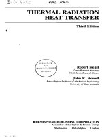
Figure 7.13 Comparison of Churchill and Bernstein’s correla-
tion with data by many workers from several countries for heat
transfer during cross flow over a cylinder. (See [7.24] for data
sources.) Fluids include air, water, and sodium, with both q
w
and T
w
constant.
All properties in eqns. (7.65)to(7.68) are to be evaluated at a film tem-
perature T
f
= (T
w
+T
∞
)

2.
Example 7.7
An electric resistance wire heater 0.0001 m in diameter is placed per-
pendicular to an air flow. It holds a temperature of 40
◦
Cina20
◦
C air
flow while it dissipates 17.8W/m of heat to the flow. How fast is the
air flowing?
Solution.
h = (17.8W/m)


[π(0.0001 m)(40 − 20)K]= 2833
W/m
2
K. Therefore, Nu
D
= 2833(0.0001)/0.0264 = 10.75, where we
have evaluated k = 0.0264 at T = 30
◦
C. We now want to find the Re
D
for which Nu
D
is 10.75. From Fig. 7.13 we see that Re
D
is around 300
380 Forced convection in a variety of configurations §7.6
when the ordinate is on the order of 10. This means that we can solve
eqn. (7.66) to get an accurate value of Re
D
:
Re
D
=



(
Nu
D
−0.3)



1 +

0.4
Pr

2/3

1/4

0.62 Pr
1/3



2
but Pr = 0.71, so
Re
D
=



(10.75 −0.3)


1 +

0.40

0.71

2/3

1/4

0.62(0.71)
1/3



2
= 463
Then
u
∞
=
ν
D
Re
D
=

1.596 ×10
−5
10
−4

463 = 73.9m/s
The data scatter in Re

D
is quite small—less than 10%, it would
appear—in Fig. 7.13. Therefore, this method can be used to measure
local velocities with good accuracy. If the device is calibrated, its
accuracy is improved further. Such an air speed indicator is called a
hot-wire anemometer, as discussed further in Problem 7.45.
Heat transfer during flow across tube bundles
A rod or tube bundle is an arrangement of parallel cylinders that heat, or
are being heated by, a fluid that might flow normal to them, parallel with
them, or at some angle in between. The flow of coolant through the fuel
elements of all nuclear reactors being used in this country is parallel to
the heating rods. The flow on the shell side of most shell-and-tube heat
exchangers is generally normal to the tube bundles.
Figure 7.14 shows the two basic configurations of a tube bundle in
a cross flow. In one, the tubes are in a line with the flow; in the other,
the tubes are staggered in alternating rows. For either of these configura-
tions, heat transfer data can be correlated reasonably well with power-law
relations of the form
Nu
D
= C Re
n
D
Pr
1/3
(7.69)
but in which the Reynolds number is based on the maximum velocity,
u
max
= u

av
in the narrowest transverse area of the passage
§7.6 Heat transfer during cross flow over cylinders 381
Figure 7.14 Aligned and staggered tube rows in tube bundles.
Thus, the Nusselt number based on the average heat transfer coefficient
over any particular isothermal tube is
Nu
D
=
hD
k
and Re
D
=
u
max
D
ν
Žukauskas at the Lithuanian Academy of Sciences Institute in Vilnius
has written two comprehensive review articles on tube-bundle heat trans-
382 Forced convection in a variety of configurations §7.6
fer [7.26, 7.27]. In these he summarizes his work and that of other Soviet
workers, together with earlier work from the West. He was able to corre-
late data over very large ranges of Pr, Re
D
, S
T
/D, and S
L
/D (see Fig. 7.14)

with an expression of the form
Nu
D
= Pr
0.36
(
Pr/Pr
w
)
n
fn
(
Re
D
)
with n =



0 for gases
1
4
for liquids
(7.70)
where properties are to be evaluated at the local fluid bulk temperature,
except for Pr
w
, which is evaluated at the uniform tube wall temperature,
T
w

.
The function fn(Re
D
) takes the following form for the various circum-
stances of flow and tube configuration:
100  Re
D
 10
3
:
aligned rows: fn
(
Re
D
)
= 0.52 Re
0.5
D
(7.71a)
staggered rows: fn
(
Re
D
)
= 0.71 Re
0.5
D
(7.71b)
10
3

 Re
D
 2 ×10
5
:
aligned rows: fn
(
Re
D
)
= 0.27 Re
0.63
D
,S
T
/S
L
 0.7
(7.71c)
For S
T
/S
L
< 0.7, heat exchange is much less effective.
Therefore, aligned tube bundles are not designed in this
range and no correlation is given.
staggered rows: fn
(
Re
D

)
= 0.35
(
S
T
/S
L
)
0.2
Re
0.6
D
,
S
T
/S
L
 2 (7.71d)
fn
(
Re
D
)
= 0.40 Re
0.6
D
,S
T
/S
L

> 2 (7.71e)
Re
D
> 2 ×10
5
:
aligned rows: fn
(
Re
D
)
= 0.033 Re
0.8
D
(7.71f)
staggered rows: fn
(
Re
D
)
= 0.031
(
S
T
/S
L
)
0.2
Re
0.8

D
,
Pr > 1 (7.71g)
Nu
D
= 0.027
(
S
T
/S
L
)
0.2
Re
0.8
D
,
Pr = 0.7 (7.71h)
All of the preceding relations apply to the inner rows of tube bundles.
The heat transfer coefficient is smaller in the rows at the front of a bundle,
§7.6 Heat transfer during cross flow over cylinders 383
Figure 7.15 Correction for the heat
transfer coefficients in the front rows of a
tube bundle [7.26].
facing the oncoming flow. The heat transfer coefficient can be corrected
so that it will apply to any of the front rows using Fig. 7.15.
Early in this chapter we alluded to the problem of predicting the heat
transfer coefficient during the flow of a fluid at an angle other than 90
◦
to the axes of the tubes in a bundle. Žukauskas provides the empirical

corrections in Fig. 7.16 to account for this problem.
The work of Žukauskas does not extend to liquid metals. However,
Kalish and Dwyer [7.28] present the results of an experimental study of
heat transfer to the liquid eutectic mixture of 77.2% potassium and 22.8%
sodium (called NaK). NaK is a fairly popular low-melting-point metallic
coolant which has received a good deal of attention for its potential use in
certain kinds of nuclear reactors. For isothermal tubes in an equilateral
triangular array, as shown in Fig. 7.17, Kalish and Dwyer give
Nu
D
=

5.44 +0.228 Pe
0.614





C
P −D
P

sin φ + sin
2
φ
1 +sin
2
φ


(7.72)
Figure 7.16 Correction for the heat
transfer coefficient in flows that are not
perfectly perpendicular to heat exchanger
tubes [7.26].
384 Forced convection in a variety of configurations §7.7
Figure 7.17 Geometric correction for
the Kalish-Dwyer equation (7.72).
where
• φ is the angle between the flow direction and the rod axis.
• P is the “pitch” of the tube array, as shown in Fig. 7.17, and D is
the tube diameter.
• C is the constant given in Fig. 7.17.
• Pe
D
is the Péclét number based on the mean flow velocity through
the narrowest opening between the tubes.
• For the same uniform heat flux around each tube, the constants in
eqn. (7.72) change as follows: 5.44 becomes 4.60; 0.228 becomes
0.193.
7.7 Other configurations
At the outset, we noted that this chapter would move further and further
beyond the reach of analysis in the heat convection problems that it dealt
with. However, we must not forget that even the most completely em-
pirical relations in Section 7.6 were devised by people who were keenly
aware of the theoretical framework into which these relations had to fit.
Notice, for example, that eqn. (7.66) reduces to Nu
D
∝


Pe
D
as Pr be-
comes small. That sort of theoretical requirement did not just pop out
of a data plot. Instead, it was a consideration that led the authors to
select an empirical equation that agreed with theory at low Pr.
Thus, the theoretical considerations in Chapter 6 guide us in correlat-
ing limited data in situations that cannot be analyzed. Such correlations
§7.7 Other configurations 385
can be found for all kinds of situations, but all must be viewed critically.
Many are based on limited data, and many incorporate systematic errors
of one kind or another.
In the face of a heat transfer situation that has to be predicted, one
can often find a correlation of data from similar systems. This might in-
volve flow in or across noncircular ducts; axial flow through tube or rod
bundles; flow over such bluff bodies as spheres, cubes, or cones; or flow
in circular and noncircular annuli. The Handbook of Heat Transfer [7.29],
the shelf of heat transfer texts in your library, or the journals referred
to by the Engineering Index are among the first places to look for a cor-
relation curve or equation. When you find a correlation, there are many
questions that you should ask yourself:
• Is my case included within the range of dimensionless parameters
upon which the correlation is based, or must I extrapolate to reach
my case?
• What geometric differences exist between the situation represented
in the correlation and the one I am dealing with? (Such elements as
these might differ:
(a) inlet flow conditions;
(b) small but important differences in hardware, mounting brack-
ets, and so on;

(c) minor aspect ratio or other geometric nonsimilarities
• Does the form of the correlating equation that represents the data,
if there is one, have any basis in theory? (If it is only a curve fit to
the existing data, one might be unjustified in using it for more than
interpolation of those data.)
• What nuisance variables might make our systems different? For
example:
(a) surface roughness;
(b) fluid purity;
(c) problems of surface wetting
• To what extend do the data scatter around the correlation line? Are
error limits reported? Can I actually see the data points? (In this
regard, you must notice whether you are looking at a correlation
386 Chapter 7: Forced convection in a variety of configurations
on linear or logarithmic coordinates. Errors usually appear smaller
than they really are on logarithmic coordinates. Compare, for ex-
ample, the data of Figs. 8.3 and 8.10.)
• Are the ranges of physical variables large enough to guarantee that
I can rely on the correlation for the full range of dimensionless
groups that it purports to embrace?
• Am I looking at a primary or secondary source (i.e., is this the au-
thor’s original presentation or someone’s report of the original)? If
it is a secondary source, have I been given enough information to
question it?
• Has the correlation been signed by the persons who formulated it?
(If not, why haven’t the authors taken responsibility for the work?)
Has it been subjected to critical review by independent experts in
the field?
Problems
7.1 Prove that in fully developed laminar pipe flow, (−dp/dx)R

2

4µ
is twice the average velocity in the pipe. To do this, set the
mass flow rate through the pipe equal to (ρu
av
)(area).
7.2 A flow of air at 27
◦
C and 1 atm is hydrodynamically fully de-
veloped ina1cmI.D. pipe with u
av
= 2m/s. Plot (to scale) T
w
,
q
w
, and T
b
as a function of the distance x after T
w
is changed
or q
w
is imposed:
a. In the case for which T
w
= 68.4
◦
C = constant.

b. In the case for which q
w
= 378 W/m
2
= constant.
Indicate x
e
t
on your graphs.
7.3 Prove that C
f
is 16/Re
D
in fully developed laminar pipe flow.
7.4 Air at 200
◦
C flows at 4 m/sovera3cmO.D. pipe that is kept
at 240
◦
C. (a) Find h. (b) If the flow were pressurized water at
200
◦
C, what velocities would give the same h, the same Nu
D
,
and the same Re
D
? (c) If someone asked if you could model
the water flow with an air experiment, how would you answer?
[u

∞
= 0.0156 m/s for same Nu
D
.]
Problems 387
7.5 Compare the h value calculated in Example 7.3 with those
calculated from the Dittus-Boelter, Colburn, and Sieder-Tate
equations. Comment on the comparison.
7.6 Water at T
b
local
= 10
◦
C flows ina3cmI.D. pipe at 1 m/s. The
pipe walls are kept at 70
◦
C and the flow is fully developed.
Evaluate h and the local value of dT
b
/dx at the point of inter-
est. The relative roughness is 0.001.
7.7 Water at 10
◦
C flows overa3cmO.D. cylinder at 70
◦
C. The
velocity is 1 m/s. Evaluate
h.
7.8 Consider the hot wire anemometer in Example 7.7. Suppose
that 17.8W/m is the constant heat input, and plot u

∞
vs. T
wire
over a reasonable range of variables. Must you deal with any
changes in the flow regime over the range of interest?
7.9 Water at 20
◦
C flows at 2 m/s over a 2 m length of pipe, 10 cm in
diameter, at 60
◦
C. Compare h for flow normal to the pipe with
that for flow parallel to the pipe. What does the comparison
suggest about baffling in a heat exchanger?
7.10 A thermally fully developed flow of NaK in a 5 cm I.D. pipe
moves at u
av
= 8m/s. If T
b
= 395
◦
C and T
w
is constant at
403
◦
C, what is the local heat transfer coefficient? Is the flow
laminar or turbulent?
7.11 Water entersa7cmI.D. pipe at 5
◦
C and moves through it at an

average speed of 0.86 m/s. The pipe wall is kept at 73
◦
C. Plot
T
b
against the position in the pipe until (T
w
− T
b
)/68 = 0.01.
Neglect the entry problem and consider property variations.
7.12 Air at 20
◦
C flows over a very large bank of 2 cm O.D. tubes
that are kept at 100
◦
C. The air approaches at an angle 15
◦
off
normal to the tubes. The tube array is staggered, with S
L
=
3.5cmandS
T
= 2.8 cm. Find h on the first tubes and on the
tubes deep in the array if the air velocity is 4.3m/s before it
enters the array. [
h
deep
= 118 W/m

2
K.]
7.13 Rework Problem 7.11 using a single value of
h evaluated at
3(73 − 5)/4 = 51
◦
C and treating the pipe as a heat exchan-
ger. At what length would you judge that the pipe is no longer
efficient as an exchanger? Explain.
388 Chapter 7: Forced convection in a variety of configurations
7.14 Go to the periodical engineering literature in your library. Find
a correlation of heat transfer data. Evaluate the applicability of
the correlation according to the criteria outlined in Section 7.7.
7.15 Water at 24
◦
C flows at 0.8m/s in a smooth, 1.5 cm I.D. tube
that is kept at 27
◦
C. The system is extremely clean and quiet,
and the flow stays laminar until a noisy air compressor is turned
on in the laboratory. Then it suddenly goes turbulent. Calcu-
late the ratio of the turbulent h to the laminar h.[h
turb
=
4429 W/m
2
K.]
7.16 Laboratory observations of heat transfer during the forced flow
of air at 27
◦

C over a bluff body, 12 cm wide, kept at 77
◦
C yield
q = 646 W/m
2
when the air moves 2 m/s and q = 3590 W/m
2
when it moves 18 m/s. In another test, everything else is the
same, but now 17
◦
C water flowing 0.4m/s yields 131,000 W/m
2
.
The correlations in Chapter 7 suggest that, with such limited
data, we can probably create a fairly good correlation in the
form:
Nu
L
= CRe
a
Pr
b
. Estimate the constants C, a, and b by
cross-plotting the data on log-log paper.
7.17 Air at 200 psia flows at 12 m/s in an 11 cm I.D. duct. Its bulk
temperature is 40
◦
C and the pipe wall is at 268
◦
C. Evaluate h

if ε/D = 0.00006.
7.18 How does
h during cross flow over a cylindrical heat vary with
the diameter when Re
D
is very large?
7.19 Air enters a 0.8 cm I.D. tube at 20
◦
C with an average velocity
of 0.8m/s. The tube wall is kept at 40
◦
C. Plot T
b
(x) until it
reaches 39
◦
C. Use properties evaluated at [(20 +40)/2]
◦
C for
the whole problem, but report the local error in h at the end
to get a sense of the error incurred by the simplification.
7.20 Write Re
D
in terms of
˙
m in pipe flow and explain why this rep-
resentation could be particularly useful in dealing with com-
pressible pipe flows.
7.21 NaK at 394
◦

C flows at 0.57 m/s across a 1.82 m length of
0.036 m O.D. tube. The tube is kept at 404
◦
C. Find h and the
heat removal rate from the tube.
7.22 Verify the value of h specified in Problem 3.22.
Problems 389
7.23 Check the value of h given in Example 7.3 by using Reynolds’s
analogy directly to calculate it. Which h do you deem to be in
error, and by what percent?
7.24 A homemade heat exchanger consists of a copper plate, 0.5 m
square, with 201.5 cm I.D. copper tubes soldered to it. The
ten tubes on top are evenly spaced across the top and parallel
with two sides. The ten on the bottom are also evenly spaced,
but they run at 90
◦
to the top tubes. The exchanger is used to
cool methanol flowing at 0.48 m/s in the tubes from an initial
temperature of 73
◦
C, using water flowing at 0.91 m/s and en-
tering at 7
◦
C. What is the temperature of the methanol when
it is mixed in a header on the outlet side? Make a judgement
of the heat exchanger.
7.25 Given that
Nu
D
= 12.7at(2/Gz) = 0.004, evaluate Nu

D
at
(2/Gz) = 0.02 numerically, using Fig. 7.4. Compare the result
with the value you read from the figure.
7.26 Report the maximum percent scatter of data in Fig. 7.13. What
is happening in the fluid flow when the scatter is worst?
7.27 Water at 27
◦
C flows at 2.2m/s in a 0.04 m I.D. thin-walled
pipe. Air at 227
◦
C flows across it at 7.6m/s. Find the pipe
wall temperature.
7.28 Freshly painted aluminum rods, 0.02 m in diameter, are with-
drawn from a drying oven at 150
◦
C and cooled ina3m/s cross
flow of air at 23
◦
C. How long will it take to cool them to 50
◦
C
so that they can be handled?
7.29 At what speed, u
∞
, must 20
◦
C air flow across an insulated
tube before the insulation on it will do any good? The tube is
at 60

◦
C and is 6 mm in diameter. The insulation is 12 mm in
diameter, with k = 0.08 W/m·K. (Notice that we do not ask for
the u
∞
for which the insulation will do the most harm.)
7.30 Water at 37
◦
C flows at 3 m/s across at 6 cm O.D. tube that is
held at 97
◦
C. In a second configuration, 37
◦
C water flows at an
average velocity of 3 m/s through a bundle of 6 cm O.D. tubes
that are held at 97
◦
C. The bundle is staggered, with S
T
/S
L
= 2.
Compare the heat transfer coefficients for the two situations.
390 Chapter 7: Forced convection in a variety of configurations
7.31 It is proposed to cool 64
◦
C air as it flows, fully developed,
ina1mlength of 8 cm I.D. smooth, thin-walled tubing. The
coolant is Freon 12 flowing, fully developed, in the opposite di-
rection, in eight smooth 1 cm I.D. tubes equally spaced around

the periphery of the large tube. The Freon enters at −15
◦
C and
is fully developed over almost the entire length. The average
speeds are 30 m/s for the air and 0.5m/s for the Freon. De-
termine the exiting air temperature, assuming that soldering
provides perfect thermal contact between the entire surface of
the small tubes and the surface of the large tube. Criticize the
heat exchanger design and propose some design improvement.
7.32 Evaluate
Nu
D
using Giedt’s data for air flowing over a cylinder
at Re
D
= 140, 000. Compare your result with the appropriate
correlation and with Fig. 7.13.
7.33 A 25 mph wind blows across a 0.25 in. telephone line. What is
the pitch of the hum that it emits?
7.34 A large Nichrome V slab, 0.2 m thick, has two parallel 1 cm I.D.
holes drilled through it. Their centers are 8 cm apart. One
carries liquid CO
2
at 1.2m/s from a −13
◦
C reservoir below.
The other carries methanol at 1.9m/s from a 47
◦
C reservoir
above. Take account of the intervening Nichrome and compute

the heat transfer. Need we worry about the CO
2
being warmed
up by the methanol?
7.35 Consider the situation described in Problem 4.38 but suppose
that you do not know
h. Suppose, instead, that you know there
isa10m/s cross flow of 27
◦
C air over the rod. Then rework
the problem.
7.36 A liquid whose properties are not known flows across a 40 cm
O.D. tube at 20 m/s. The measured heat transfer coefficient is
8000 W/m
2
K. We can be fairly confident that Re
D
is very large
indeed. What would
h be if D were 53 cm? What would
h be
if u
∞
were 28 m/s?
7.37 Water flows at 4 m/s, at a temperature of 100
◦
C,ina6cmI.D.
thin-walled tube witha2cmlayer of 85% magnesia insulation
on it. The outside heat transfer coefficient is 6 W/m
2

K, and the
outside temperature is 20
◦
C. Find: (a) U based on the inside
Problems 391
area, (b) Q W/m, and (c) the temperature on either side of the
insulation.
7.38 Glycerin is added to water in a mixing tank at 20
◦
C. The mix-
ture discharges througha4mlength of 0.04 m I.D. tubing
under a constant 3 m head. Plot the discharge rate in m
3
/hr
as a function of composition.
7.39 Plot
h as a function of composition for the discharge pipe in
Problem 7.38. Assume a small temperature difference.
7.40 Rework Problem 5.40 without assuming the Bi number to be
very large.
7.41 Water enters a 0.5 cm I.D. pipe at 24
◦
C. The pipe walls are held
at 30
◦
C. Plot T
b
against distance from entry if u
av
is 0.27 m/s,

neglecting entry behavior in your calculation. (Indicate the en-
try region on your graph, however.)
7.42 Devise a numerical method to find the velocity distribution
and friction factor for laminar flow in a square duct of side
length a. Set up a square grid of size N by N and solve the
difference equations by hand for N = 2, 3, and 4. Hint: First
show that the velocity distribution is given by the solution to
the equation
∂
2
u
∂x
2
+
∂
2
u
∂y
2
= 1
where u = 0 on the sides of the square and we define
u =
u

[(a
2
/µ)(dp/dz)], x = (x/a), and y = (y/a). Then show
that the friction factor, f [eqn. (7.34)], is given by
f =
−2

ρu
av
a
µ

udxdy
Note that the area integral can be evaluated as

u/N
2
.
7.43 Chilled air at 15
◦
C enters a horizontal duct at a speed of 1 m/s.
The duct is made of thin galvanized steel and is not insulated.
A 30 m section of the duct runs outdoors through humid air
at 30
◦
C. Condensation of moisture on the outside of the duct
is undesirable, but it will occur if the duct wall is at or below
392 Chapter 7: Forced convection in a variety of configurations
the dew point temperature of 20
◦
C. For this problem, assume
that condensation rates are so low that their thermal effects
can be ignored.
a. Suppose that the duct’s square cross-section is 0.3 m by
0.3 m and the effective outside heat transfer coefficient
is 5 W/m
2

K in still air. Determine whether condensation
occurs.
b. The single duct is replaced by four circular horizontal
ducts, each 0.17 m in diameter. The ducts are parallel
to one another in a vertical plane with a center-to-center
separation of 0.5 m. Each duct is wrapped with a layer
of fiberglass insulation 6 cm thick (k
i
= 0.04 W/m·K) and
carries air at the same inlet temperature and speed as be-
fore. If a 15 m/s wind blows perpendicular to the plane
of the circular ducts, find the bulk temperature of the air
exiting the ducts.
7.44 An x-ray “monochrometer” is a mirror that reflects only a sin-
gle wavelength from a broadband beam of x-rays. Over 99%
of the beam’s energy arrives on other wavelengths and is ab-
sorbed creating a high heat flux on part of the surface of the
monochrometer. Consider a monochrometer made from a sil-
icon block 10 mm long and 3 mm by 3 mm in cross-section
which absorbs a flux of 12.5 W/mm
2
over an area of 6 mm
2
on
one face (a heat load of 75 W). To control the temperature, it
is proposed to pump liquid nitrogen through a circular chan-
nel bored down the center of the silicon block. The channel is
10 mm long and 1 mm in diameter. LN
2
enters the channel at

80 K and a pressure of 1.6 MPa (T
sat
= 111.5 K). The entry to
this channel is a long, straight, unheated passage of the same
diameter.
a. For what range of mass flow rates will the LN
2
have a bulk
temperature rise of less than a 1.5 K over the length of the
channel?
b. At your minimum flow rate, estimate the maximum wall
temperature in the channel. As a first approximation, as-
sume that the silicon conducts heat well enough to dis-
tribute the 75 W heat load uniformly over the channel
References 393
surface. Could boiling occur in the channel? Discuss the
influence of entry length and variable property effects.
7.45 Turbulent fluid velocities are sometimes measured with a con-
stant temperature hot-wire anemometer, which consists of a
long, fine wire (typically platinum, 4µm in diameter and 1.25
mm long) supported between two much larger needles. The
needles are connected to an electronic bridge circuit which
electrically heats the wire while adjusting the heating voltage,
V
w
, so that the wire’s temperature — and thus its resistance,
R
w
— stays constant. The electrical power dissipated in the
wire, V

2
w
/R
w
, is convected away at the surface of the wire. An-
alyze the heat loss from the wire to show
V
2
w
= (T
wire
−T
flow
)

A +Bu
1/2

where u is the instantaneous flow speed perpendicular to the
wire. Assume that u is between 2 and 100 m/s and that the
fluid is an isothermal gas. The constants A and B depend on
properties, dimensions, and resistance; they are usually found
by calibration of the anemometer. This result is called King’s
law.
7.46 (a) Show that the Reynolds number for a circular tube may be
written in terms of the mass flow rate as Re
D
= 4
˙
m


πµD.
(b) Show that this result does not apply to a noncircular tube,
specifically Re
D
h
≠ 4
˙
m

πµD
h
.
References
[7.1] F. M. White. Viscous Fluid Flow. McGraw-Hill Book Company, New
York, 1974.
[7.2] S. S. Mehendale, A. M. Jacobi, and R. K. Shah. Fluid flow and heat
transfer at micro- and meso-scales with application to heat ex-
changer design. Appl. Mech. Revs., 53(7):175–193, 2000.
[7.3] W. M. Kays and M. E. Crawford. Convective Heat and Mass Transfer.
McGraw-Hill Book Company, New York, 3rd edition, 1993.
394 Chapter 7: Forced convection in a variety of configurations
[7.4] R. K. Shah and M. S. Bhatti. Laminar convective heat transfer
in ducts. In S. Kakaç, R. K. Shah, and W. Aung, editors, Hand-
book of Single-Phase Convective Heat Transfer, chapter 3. Wiley-
Interscience, New York, 1987.
[7.5] R. K. Shah and A. L. London. Laminar Flow Forced Convection in
Ducts. Academic Press, Inc., New York, 1978. Supplement 1 to the
series Advances in Heat Transfer.
[7.6] L. Graetz. Über die wärmeleitfähigkeit von flüssigkeiten. Ann.

Phys., 25:337, 1885.
[7.7] S. R. Sellars, M. Tribus, and J. S. Klein. Heat transfer to laminar
flow in a round tube or a flat plate—the Graetz problem extended.
Trans. ASME, 78:441–448, 1956.
[7.8] M. S. Bhatti and R. K. Shah. Turbulent and transition flow convec-
tive heat transfer in ducts. In S. Kakaç, R. K. Shah, and W. Aung,
editors, Handbook of Single-Phase Convective Heat Transfer, chap-
ter 4. Wiley-Interscience, New York, 1987.
[7.9] F. Kreith. Principles of Heat Transfer. Intext Press, Inc., New York,
3rd edition, 1973.
[7.10] A. P. Colburn. A method of correlating forced convection heat
transfer data and a comparison with fluid friction. Trans. AIChE,
29:174, 1933.
[7.11] L. M. K. Boelter, V. H. Cherry, H. A. Johnson, and R. C. Martinelli.
Heat Transfer Notes. McGraw-Hill Book Company, New York, 1965.
[7.12] E. N. Sieder and G. E. Tate. Heat transfer and pressure drop of
liquids in tubes. Ind. Eng. Chem., 28:1429, 1936.
[7.13] B. S. Petukhov. Heat transfer and friction in turbulent pipe flow
with variable physical properties. In T.F. Irvine, Jr. and J. P. Hart-
nett, editors, Advances in Heat Transfer, volume 6, pages 504–564.
Academic Press, Inc., New York, 1970.
[7.14] V. Gnielinski. New equations for heat and mass transfer in turbu-
lent pipe and channel flow. Int. Chemical Engineering, 16:359–368,
1976.
References 395
[7.15] S. E. Haaland. Simple and explicit formulas for the friction factor
in turbulent pipe flow. J. Fluids Engr., 105:89–90, 1983.
[7.16] T. S. Ravigururajan and A. E. Bergles. Development and verifica-
tion of general correlations for pressure drop and heat transfer
in single-phase turbulent flow in enhanced tubes. Exptl. Thermal

Fluid Sci., 13:55–70, 1996.
[7.17] R. L. Webb. Enhancement of single-phase heat transfer. In S. Kakaç,
R. K. Shah, and W. Aung, editors, Handbook of Single-Phase Con-
vective Heat Transfer, chapter 17. Wiley-Interscience, New York,
1987.
[7.18] B. Lubarsky and S. J. Kaufman. Review of experimental investiga-
tions of liquid-metal heat transfer. NACA Tech. Note 3336, 1955.
[7.19] C. B. Reed. Convective heat transfer in liquid metals. In S. Kakaç,
R. K. Shah, and W. Aung, editors, Handbook of Single-Phase Convec-
tive Heat Transfer, chapter 8. Wiley-Interscience, New York, 1987.
[7.20] R. A. Seban and T. T. Shimazaki. Heat transfer to a fluid flowing
turbulently in a smooth pipe with walls at a constant temperature.
Trans. ASME, 73:803, 1951.
[7.21] R. N. Lyon, editor. Liquid Metals Handbook. A.E.C. and Dept. of the
Navy, Washington, D.C., 3rd edition, 1952.
[7.22] J. H. Lienhard. Synopsis of lift, drag, and vortex frequency data
for rigid circular cylinders. Bull. 300. Wash. State Univ., Pullman,
1966.
[7.23] W. H. Giedt. Investigation of variation of point unit-heat-transfer
coefficient around a cylinder normal to an air stream. Trans. ASME,
71:375–381, 1949.
[7.24] S. W. Churchill and M. Bernstein. A correlating equation for forced
convection from gases and liquids to a circular cylinder in cross-
flow. J. Heat Transfer, Trans. ASME, Ser. C, 99:300–306, 1977.
[7.25] S. Nakai and T. Okazaki. Heat transfer from a horizontal circular
wire at small Reynolds and Grashof numbers—1 pure convection.
Int. J. Heat Mass Transfer, 18:387–396, 1975.
396 Chapter 7: Forced convection in a variety of configurations
[7.26] A. Žukauskas. Heat transfer from tubes in crossflow. In T.F. Irvine,
Jr. and J. P. Hartnett, editors, Advances in Heat Transfer, volume 8,

pages 93–160. Academic Press, Inc., New York, 1972.
[7.27] A. Žukauskas. Heat transfer from tubes in crossflow. In T. F.
Irvine, Jr. and J. P. Hartnett, editors, Advances in Heat Transfer,
volume 18, pages 87–159. Academic Press, Inc., New York, 1987.
[7.28] S. Kalish and O. E. Dwyer. Heat transfer to NaK flowing through
unbaffled rod bundles. Int. J. Heat Mass Transfer, 10:1533–1558,
1967.
[7.29] W. M. Rohsenow, J. P. Hartnett, and Y. I. Cho, editors. Handbook
of Heat Transfer. McGraw-Hill, New York, 3rd edition, 1998.
8. Natural convection in single-
phase fluids and during film
condensation
There is a natural place for everything to seek, as:
Heavy things go downward, fire upward, and rivers to the sea.
The Anatomy of Melancholy, R. Burton, 1621
8.1 Scope
The remaining convection mechanisms that we deal with are to a large
degree gravity-driven. Unlike forced convection, in which the driving
force is external to the fluid, these so-called natural convection processes
are driven by body forces exerted directly within the fluid as the result
of heating or cooling. Two such mechanisms that are rather alike are:
• Natural convection. When we speak of natural convection without
any qualifying words, we mean natural convection in a single-phase
fluid.
• Film condensation. This natural convection process has much in
common with single-phase natural convection.
We therefore deal with both mechanisms in this chapter. The govern-
ing equations are developed side by side in two brief opening sections.
Then each mechanism is developed independently in Sections 8.3 and
8.4 and in Section 8.5, respectively.

Chapter 9 deals with other natural convection heat transfer processes
that involve phase change—for example:
397
398 Natural convection in single-phase fluids and during film condensation §8.2
• Nucleate boiling. This heat transfer process is highly disordered as
opposed to the processes described in Chapter 8.
• Film boiling. This is so similar to film condensation that it is usually
treated by simply modifying film condensation predictions.
• Dropwise condensation. This bears some similarity to nucleate boil-
ing.
8.2 The nature of the problems of film condensation
and of natural convection
Description
The natural convection problem is sketched in its simplest form on the
left-hand side of Fig. 8.1. Here we see a vertical isothermal plate that
cools the fluid adjacent to it. The cooled fluid sinks downward to form a
b.l. The figure would be inverted if the plate were warmer than the fluid
next to it. Then the fluid would buoy upward.
On the right-hand side of Fig. 8.1 is the corresponding film conden-
sation problem in its simplest form. An isothermal vertical plate cools
an adjacent vapor, which condenses and forms a liquid film on the wall.
1
The film is normally very thin and it flows off, rather like a b.l., as the
figure suggests. While natural convection can carry fluid either upward
or downward, a condensate film can only move downward. The temper-
ature in the film rises from T
w
at the cool wall to T
sat
at the outer edge

of the film.
In both problems, but particularly in film condensation, the b.l. and
the film are normally thin enough to accommodate the b.l. assumptions
[recall the discussion following eqn. (6.13)]. A second idiosyncrasy of
both problems is that δ and δ
t
are closely related. In the condensing
film they are equal, since the edge of the condensate film forms the edge
of both b.l.’s. In natural convection, δ and δ
t
are approximately equal
when Pr is on the order of unity or less, because all cooled (or heated)
fluid must buoy downward (or upward). When Pr is large, the cooled (or
heated) fluid will fall (or rise) and, although it is all very close to the wall,
this fluid, with its high viscosity, will also drag unheated liquid with it.
1
It might instead condense into individual droplets, which roll of without forming
into a film. This process, called dropwise condensation, is dealt with in Section 9.9.
§8.2 The nature of the problems of film condensation and of natural convection 399
Figure 8.1 The convective boundary layers for natural con-
vection and film condensation. In both sketches, but particu-
larly in that for film condensation, the y-coordinate has been
stretched.
In this case, δ can exceed δ
t
. We deal with cases for which δ  δ
t
in the
subsequent analysis.
Governing equations

To describe laminar film condensation and laminar natural convection,
we must add a gravity term to the momentum equation. The dimensions
of the terms in the momentum equation should be examined before we
do this. Equation (6.13) can be written as

u
∂u
∂x
+v
∂u
∂y

m
s
2
  
=
kg·m
kg·s
2
=
N
kg
=−
1
ρ
dp
dx
m
3

kg
N
m
2
·m

 
=
N
kg
+ν
∂
2
u
∂y
2
m
2
s
m
s ·m
2
  
=
m
s
2
=
N
kg

where ∂p/∂x  dp/dx in the b.l. and where µ  constant. Thus, every
term in the equation has units of acceleration or (equivalently) force per
unit mass. The component of gravity in the x-direction therefore enters
400 Natural convection in single-phase fluids and during film condensation §8.2
the momentum balance as (+g). This is because x and g point in the
same direction. Gravity would enter as −g if it acted opposite the x-
direction.
u
∂u
∂x
+v
∂u
∂y
=−
1
ρ
dp
dx
+g +ν
∂
2
u
∂y
2
(8.1)
In the two problems at hand, the pressure gradient is the hydrostatic
gradient outside the b.l. Thus,
dp
dx
= ρ

∞
g

 
natural
convection
dp
dx
= ρ
g
g

 
film
condensation
(8.2)
where ρ
∞
is the density of the undisturbed fluid and ρ
g
(and ρ
f
below)
are the saturated vapor and liquid densities. Equation (8.1) then becomes
u
∂u
∂x
+v
∂u
∂y

=

1 −
ρ
∞
ρ

g + ν
∂
2
u
∂y
2
for natural convection (8.3)
u
∂u
∂x
+v
∂u
∂y
=

1 −
ρ
g
ρ
f

g + ν
∂

2
u
∂y
2
for film condensation (8.4)
Two boundary conditions, which apply to both problems, are
u

y = 0

= 0
the no-slip condition
v

y = 0

= 0 no flow into the wall

(8.5a)
The third b.c. is different for the film condensation and natural convec-
tion problems:
∂u
∂y





y=δ
= 0

condensation:
no shear at the edge of the film
u

y = δ

= 0
natural convection:
undisturbed fluid outside the b.l.











(8.5b)
The energy equation for either of the two cases is eqn. (6.40):
u
∂T
∂x
+v
∂T
∂y
= α
∂

2
T
∂y
2
We leave the identification of the b.c.’s for temperature until later.
The crucial thing we must recognize about the momentum equation
at the moment is that it is coupled to the energy equation. Let us consider
how that occurs:
§8.3 Laminar natural convection on a vertical isothermal surface 401
In natural convection: The velocity, u, is driven by buoyancy, which is
reflected in the term (1 −ρ
∞
/ρ)g in the momentum equation. The
density, ρ = ρ(T), varies with T , so it is impossible to solve the
momentum and energy equations independently of one another.
In film condensation: The third boundary condition (8.5b) for the mo-
mentum equation involves the film thickness, δ. But to calculate δ
we must make an energy balance on the film to find out how much
latent heat—and thus how much condensate—it has absorbed. This
will bring (T
sat
−T
w
) into the solution of the momentum equation.
Recall that the boundary layer on a flat surface, during forced convec-
tion, was easy to analyze because the momentum equation could be
solved completely before any consideration of the energy equation was
attempted. We do not have that advantage in predicting natural convec-
tion or film condensation.
8.3 Laminar natural convection on a vertical

isothermal surface
Dimensional analysis and experimental data
Before we attempt a dimensional analysis of the natural convection prob-
lem, let us simplify the buoyancy term, (ρ −ρ
∞
)g

ρ, in the momentum
equation (8.3). The equation was derived for incompressible flow, but we
modified it by admitting a small variation of density with temperature in
this term only. Now we wish to eliminate (ρ −ρ
∞
) in favor of (T −T
∞
)
with the help of the coefficient of thermal expansion, β:
β ≡
1
v
∂v
∂T




p
=−
1
ρ
∂ρ

∂T




p
−
1
ρ
ρ − ρ
∞
T − T
∞
=−

1 −ρ
∞

ρ

T − T
∞
(8.6)
where v designates the specific volume here, not a velocity component.
Figure 8.2 shows natural convection from a vertical surface that is
hotter than its surroundings. In either this case or on the cold plate
shown in Fig. 8.1, we replace (1 − ρ
∞
/ρ)g with −gβ(T − T
∞

). The sign
(see Fig. 8.2) is the same in either case. Then
u
∂u
∂x
+v
∂u
∂y
=−gβ(T − T
∞
) +ν
∂
2
u
∂y
2
(8.7)
402 Natural convection in single-phase fluids and during film condensation §8.3
Figure 8.2 Natural convection from a
vertical heated plate.
where the minus sign corresponds to plate orientation in Fig. 8.1a. This
conveniently removes ρ from the equation and makes the coupling of
the momentum and energy equations very clear.
The functional equation for the heat transfer coefficient, h, in natural
convection is therefore (cf. Section 6.4)
h or
h = fn

k, |T
w

−T
∞
|,x or L, ν, α, g, β

where L is a length that must be specified for a given problem. Notice that
while h was assumed to be independent of ∆T in the forced convection
problem (Section 6.4), the explicit appearance of (T − T
∞
) in eqn. (8.7)
suggests that we cannot make that assumption here. There are thus eight
variables in W, m, s, and
◦
C (where we again regard J as a unit independent
of N and m); so we look for 8−4 = 4 pi-groups. For
h and a characteristic
length, L, the groups may be chosen as
Nu
L
≡
hL
k
, Pr ≡
ν
α
, Π
3
≡
L
3
ν

2


g


, Π
4
≡ β |T
w
−T
∞
|=β ∆T
where we set ∆T ≡|T
w
−T
∞
|. Two of these groups are new to us:
• Π
3
≡ gL
3
/ν
2
: This characterizes the importance of buoyant forces
relative to viscous forces.
2
2
Note that gL is dimensionally the same as a velocity squared—say, u
2

. Then

Π
3
can be interpreted as a Reynolds number: uL/ν. In a laminar b.l. we recall that Nu ∝
Re
1/2
; so here we expect that Nu ∝ Π
1/4
3
.
§8.3 Laminar natural convection on a vertical isothermal surface 403
• Π
4
≡ β∆T : This characterizes the thermal expansion of the fluid.
For an ideal gas,
β =
1
v
∂
∂T

RT
p

p
=
1
T
∞

where R is the gas constant. Therefore, for ideal gases
β ∆T =
∆T
T
∞
(8.8)
It turns out that Π
3
and Π
4
(which do not bear the names of famous
people) usually appear as a product. This product is called the Grashof
(pronounced Gráhs-hoff) number,
3
Gr
L
, where the subscript designates
the length on which it is based:
Π
3
Π
4
≡ Gr
L
=
gβ∆TL
3
ν
2
(8.9)

Two exceptions in which Π
3
and Π
4
appear independently are rotating
systems (where Coriolis forces are part of the body force) and situations
in which β∆T is no longer  1 but instead approaches unity. We there-
fore expect to correlate data in most other situations with functional
equations of the form
Nu = fn(Gr, Pr) (8.10)
Another attribute of the dimensionless functional equation is that the
primary independent variable is usually the product of Gr and Pr. This
is called the Rayleigh number, Ra
L
, where the subscript designates the
length on which it is based:
Ra
L
≡ Gr
L
Pr =
gβ∆TL
3
αν
(8.11)
3
Nu, Pr, Π
3
, Π
4

, and Gr were all suggested by Nusselt in his pioneering paper on
convective heat transfer [8.1]. Grashof was a notable nineteenth-century mechanical
engineering professor who was simply given the honor of having a dimensionless group
named after him posthumously (see, e.g., [8.2]). He did not work with natural convec-
tion.