Adaptive Techniques for Dynamic Processor Optimization Theory and Practice by Alice Wang and Samuel Naffziger_3 doc

Chapter 1 Technology Challenges Motivating Adaptive Techniques 23
[20] N. Kimizuka, Y. Yasuda, T. Iwamoto*, I. Yamamoto, K. Takano, Y. Aki-
yama, and K. Imai, “Ultra-Low Standby Power (U-LSTP) 65-nm Node
CMOS Technology Utilizing HfSiON Dielectric and Body-Biasing
Scheme,” Symposium on VLSI Technology, Digest of Tech. Papers, pp.
218–219, June 2005.
Chapter 2 Technological Boundaries of Voltage
and Frequency Scaling for Power Performance
Tuning
Maurice Meijer
1
, José Pineda de Gyvez
1,2
1
NXP Semiconductors,
2
Eindhoven University of Technology
2.1 Adaptive Power Performance Tuning of ICs
The integration density of Integrated Circuits is doubling every 18 months.
Soon, advanced process generations will integrate 1 billion transistors on a
single chip. Such chips are the heart of a new generation of devices that are
changing our daily life fundamentally. Power consumption of conventional
electronic devices is a major concern because the dense devices produce a
significant amount of heat imposing constraints on circuit performance and
IC packaging. The case for portable devices is obvious, e.g. the goal is to
maximize battery time. Designing ICs for low power will be a key
practical and competitive advantage in the coming decade.
From a technological standpoint, power consumption can be reduced by
downscaling transistor dimensions. CMOS transistor scaling consists of

In this chapter, we concentrate on technological quantitative pointers for

adaptive voltage scaling (AVS) and adaptive body biasing (ABB) in
modern CMOS digital designs. In particular, we will present the power
savings that can be expected, the power-delay trade-offs that can be made,
and the implications of these techniques on present semiconductor techn-
ologies. Furthermore, we will show to which extent process-dependent
performance compensation can be used. Our presentation is a result of
extensive analyses based on test-circuits fabricated in the state-of-the-art
CMOS processes. Experimental results have been obtained for both 90nm
and 65nm CMOS technology nodes.
A. Wang, S. Naffziger (eds.), Adaptive Techniques for Dynamic Processor Optimization,
DOI: 10.1007/978-0-387-76472-6_2, © Springer Science+Business Media, LLC 2008

26 Maurice Meijer, José Pineda de Gyvez
reducing all dimensions by a factor k (≈1.4), enabling higher integration
density [1]. In the constant-field scaling scenario, the circuit speed
increases, theoretically, with the amount of scaling k. Constant-field
scaling has known benefits such as lower power per circuit, constant
power density, and power-delay product that increases by k
3
. However, for
CMOS technology, over the last 10 years, it has been impossible to scale
power supply voltage (V
DD
) while maintaining speed because of the
constraints on the threshold voltage (V
th
) [2]. Due to increasing leakage
current in scaled devices, V
th
is not lowered to avoid significant static

power consumption. Therefore, the electrical field is rising in proportion to
k resulting now in almost constant circuit power despite scaling, increased
power density by k
2
, and power-delay product improvement by a factor of
k only. In essence, the limits of a scaling process are caused by physical
effects that do not scale properly, among them are quantum-mechanical
tunneling, discrete carrier doping, and other voltage-related effects such as
the subthreshold swing, and built-in voltage and minimum voltage swings.

supply voltage
power
AVS
nom V
DD
max V
DD
min V
DD
supply voltage
power
AVS
nom V
DD
max V
DD
min V
DD

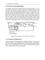
Figure 2.1 Power trends as a function of the supply voltage.

Besides technology scaling, one of the most effective ways to reduce
active power consumption is by lowering V
DD
. Ideally, quadratic power
savings are observed as displayed in Figure 2.1. V
DD
reduction can be
applied to a complete chip, but it is most effective when it is applied to local
voltage domains with own performance requirements. A common approach
is to perform dynamic supply scaling, which exploits the temporal domain to
optimize V
DD
at run-time. This technique dynamically varies both operating
frequency and supply voltage in response to workload demands. In this way,
a processing unit always operates at the desired performance level while
consuming the minimal amount of power. Two basic flavors exist, namely
dynamic voltage scaling (DVS) and adaptive voltage scaling (AVS). DVS is
Chapter 2 Technological Boundaries of Voltage and Frequency Scaling 27
an open-loop approach, and it is based on the selection of operating points
from a predefined {f,V} table. Alternatively, AVS is a closed-loop approach,
and its operating points are based only on the frequency. Software decides
on the performance required for the existing workload and selects a target
frequency. The voltage is then automatically adjusted to support this
frequency. AVS is considered as the most effective technique for achieving
power savings through V
DD
scaling.

body bias voltage

leakage
ABB
nom V
th
min V
th
max V
th
Forward biasingReverse biasing
body bias voltage
leakage
ABB
nom V
th
min V
th
max V
th
Forward biasingReverse biasing

Figure 2.2 Leakage trends as a function of body biasing.

Yet another, but complementary, approach is to adapt to the threshold
voltage of MOS devices using transistor body biasing. For NMOS, the V
th

is increased when its body–source voltage is biased to be negative. This is
referred to as reverse body biasing (RBB). Alternatively, the V
th
is reduced

when the body–source voltage is biased to be positive. This is referred to
as forward body biasing (FBB). Figure 2.2 illustrates the behavior of
leakage as a function of body biasing in modern nanometer technologies.
Body biasing can effectively reduce the leakage power of the design, by
improving its run-time performance. It is most effective when it is used in
conjunction with V
DD
scaling. Typically, body biasing is done in open-loop
to calibrate circuit frequency or leakage for setting a desired mode of
operation. Adaptive body biasing (ABB) refers to closed-loop control in
which circuit parameters, e.g. speed, are monitored, compared, and
controlled against desired values.
Not surprisingly, in recent years, the application of adaptive circuit
techniques to control either or both V
DD
and V
th
has gained increased
attention. This stems from the fact that modern electronics are hampered
by the variation of fundamental process and performance parameters such
as threshold voltage and power consumption. Design technologies such as
28 Maurice Meijer, José Pineda de Gyvez
AMD’s PowerNow! [3], Transmeta’s LongRun [4], Intel’s Enhanced
SpeedStep [5], are vivid examples of commercial ICs that use power
management based on V
DD
scaling. In addition to these commercial
accomplishments, chip demonstrators with V
DD
and V

th
scaling capabilities
have also been reported in the literature archival [6–8]. Other reported uses
of V
DD
and V
th
scaling, besides power management in processors, are in
testing [9], product binning [10], and yield tuning [11].
2.2 AVS- and ABB-Scaling Operations
As the benefits of V
DD
and V
th
scaling are known, we concentrate on
quantitative pointers for using such know-how in deep submicron
technologies. For this purpose, we have evaluated various process
technologies to determine technological boundaries for AVS and ABB when
applied to digital logic circuits. Our evaluation is based on an extensive
analysis of test-circuits fabricated in 90nm general-purpose (GP), 90nm low-
power (LP), and 65nm low-power (LP) triple-well CMOS processes.
For all three CMOS processes, we have designed a clock generator unit
(CGU) that consists of multiple independent ring-oscillators and
corresponding selection circuitry. We use these CGU designs to determine
power-performance trade-offs and leakage reduction factors with AVS and
ABB. Each ring-oscillator uses minimum-sized standard-cell inverters as
delay elements and a nand-2 gate for enabling control. The power supply
of the clock generator can be controlled externally. Body biasing is
enabled for N-well and P-well independently through triple-well isolation.
The exact same clock generator was laid out in 90nm GP and LP-CMOS

using a commercial place-and-route tool with constrained area-routing
features. The 65nm LP-CMOS clock generator was designed full-custom
using digital standard cells. Our second test-chip is a circular shift-register,
which has only been laid out in 90nm LP-CMOS. The design contains 8K
flip-flops and 50K logic gates. The logic gates are connected as delay lines
between two consecutive flip-flop stages, which have an average logic
depth of six cells. One can emulate the activity of any digital core with this
circular shift register by shifting in a sequence of zeros and ones. Like the
CGU, it has independent bias control over supply voltage, N-well and P-
well biasing. The CGU provides the clock to the shift-register. The shift-
register is used to perform correlated measurements against the CGU for
validation purposes. All measurements have been performed using a
Verigy 93K SoC test system in a controlled temperature environment. The
temperature is controlled by a Temptronic Thermostream.
Chapter 2 Technological Boundaries of Voltage and Frequency Scaling 29
Devices in 90nm GP-CMOS operate at a nominal V
DD
of 1V; their
counterparts in LP-CMOS operate at 1.2V. GP-CMOS devices exhibit a
lower V
th
than LP-CMOS devices. On average, the nominal V
th
is about
0.27V, 0.37V, and 0.43V for 90nm GP, 90nm LP, and 65nm LP-CMOS,
respectively. Since ABB enables adaptation of these nominal V
th
values, we
will show the range over which V
th

can be tuned for one of the considered
process technologies. Figure 2.3 puts into perspective V
th
versus body
biasing for 65nm LP-CMOS devices as obtained from circuit simulations.
Observe that the actual value of V
th
and its sensitivity to body bias strongly
depend on the process corner: fast, typical, or slow. For the typical NMOS
device, body biasing from 0.4V (FBB) down to –1.2V (RBB) spans over a
V
th
range of about 135mV. This range is somewhat larger for PMOS devices
(~180mV). Since RBB has a direct impact on leakage reduction, it will
become evident that this technique is not very effective because the
sensitivity of V
th
to V
BS
is small. In the next sections, we quantify the impact
of these V
th
ranges on circuit power-performance tuning.

0
0.1
0.2
0.3
0.4
0.5

0.6
0.7
-2 -1.5 -1 -0.5 0 0.5
Body-to-source voltage [V]
Threshold voltage [V]
65nm LP-CMOS
NMOS W/L=1μm/L
min
fast
typical
slow
FBB
RBB
0
0.1
0.2
0.3
0.4
0.5
0.6
0.7
0.8
-0.500.511.52
Body-to-source voltage [V]
Threshold voltage [V]
RBB
FBB
65nm LP-CMOS
PMOS W/L=1μm/L
min

fast
typical
slow

Figure 2.3 V
th
adaptation through body biasing in 65nm LP-CMOS.
Let us now briefly introduce the conventions used for the AVS and
ABB schemes. Figure 2.4 shows a graph of frequency versus power as a
function of either or both AVS and ABB. The thick line shows the nominal
trend when the supply voltage is varied from its maximum to its minimum
value. The AVS operation consists of sweeping the supply voltage while
maintaining a nominal constant body bias. The ABB is essentially the
contrary approach: the supply voltage is kept constant and the body bias is
swept. Here, it holds that frequency and power have an almost linear
negative dependence on the threshold voltage. The result is a “cloud” of
frequency–power points for a given supply voltage. Finally, AVS+ABB
corresponds to the case when both supply voltage and body biasing are
swept.

30 Maurice Meijer, José Pineda de Gyvez

power
frequency
AVS
A
V
S
+
A

B
B
ABB
min V
th
max V
th
nom V
th
nom V
DD
max V
DD
min V
DD

Figure 2.4 AVS and ABB operations.
Table 2.1 presents the voltage ranges that we employed during our
measurements. Observe that the wells were forward biased for at most
0.4V and reverse biased by 1V (GP) or 1.2V (LP). Forward biasing is
constrained by the turn-on voltage of the transistors’ body–source junction
diode. Essentially, reverse biasing is unconstrained, but high reverse
biasing voltages result in increased gate-induced drain leakage.
Table 2.1 Voltage conventions for scaling operations.

90nm GP 90nm/65nm LP
AVS
V
DD
[0.5,1.0]V [0.6,1.2]V

ABB
V
nwell
[V
DD
–0.4,V
DD
+1.0]V [V
DD
–0.4,V
DD
+1.2]V

V
pwell
[–1.0,0.4]V [–1.2,0.4]V
AVS+ABB
V
DD

V
nwell
V
pwell

[0.5,1.0]V
[V
DD
–0.4,V
DD

+1.0]V
[–1.0,0.4]V
[0.6,1.2]V
[V
DD
–0.4,V
DD
+1.2]V
[–1.2,0.4]V

In the next sections, we will illustrate how these techniques can be used
to alter the power performance of integrated circuits. Please note that in the
next sections, we will use the term ringo to refer to the ring oscillators in
the CGU.
Chapter 2 Technological Boundaries of Voltage and Frequency Scaling 31
2.3 Frequency Scaling and Tuning
In most applications, there is not always a need for peak performance. In
those cases, AVS can be used to lower the supply voltage and to slow
down the core’s computing power. In fact, operating frequency and supply
voltage for a circuit design are coupled. This relationship can be expressed
by Sakurai’s alpha-power model [12]:
()
DD
thDD
V
VV
Kf
α
−
⋅≈

(2.1)

where f is the operating frequency, K is a proportionality factor, and
α
is a
process-dependent parameter that models velocity saturation. In the case of
velocity-saturated devices, α is close to 1 and the frequency scales almost
linearly with V
DD
.

1E+6
10E+6
100E+
6
1E+9
0.5 0.6 0.7 0.8 0.9 1.0 1.1 1.2 1.3
Power supply voltage [V]
Frequency [Hz]
1E+6
10E+6
100E+6
1E+9
Frequency [Hz]
Power supply voltage [V]
ABB
maxV
th
AVS

minV
th

Figure 2.5 Frequency scaling and tuning for the 65nm LP-CMOS ringo.
Let us now investigate the frequency-scaling and tuning ranges offered
by AVS and ABB in 65nm LP-CMOS. For this purpose, we determined
the dynamic range of a 101-stage ringo that is part of the CGU test-chip.
Figure 2.5 shows the ringo frequency as a function of power supply. Each
cloud of dots is associated to a unique supply voltage. Each dot in a cloud
corresponds to a unique N-well and P-well bias combination, and the line
joining the clouds indicates the nominal trend. The ringo frequency at
nominal supply (V
DD
=1.2V) is 327MHz, and 16.2MHz at minimum supply
(V
DD
=0.6V). This results in an AVS tuning range of about 310MHz. Recall
32 Maurice Meijer, José Pineda de Gyvez

-1.2
-1.1
-1
-0.9
-0.8
-0.7
-0.6
-0.5
-0.4
-0.3
-0.2

-0.1
0
0.1
0.2
0.3
0.4
0.8
0.9
1
1.1
1.2
1.3
1.4
1.5
1.6
1.7
1.8
1.9
2
2.1
2.2
2.3
2.4
P-well bias voltage [V]
N-well bias voltage [V]
Nominal

000E+0
50E+6
100E+6

150E+6
200E+6
250E+6
300E+6
350E+6
400E+6
-1.2 -1.1 -1 -0.9 -0.8 -0.7 -0.6 -0.5 -0.4 -0.3 -0.2 -0.1 0 0.1 0.2 0.3 0.4
Well bias voltage [V]
Frequency [Hz]
V
DD
=1.2V
V
DD
=0.6V
V
DD
=0.7V
V
DD
=0.8V
V
DD
=0.9V
V
DD
=1.0V
V
DD
=1.1V

Nominal
V
nwell
=V
DD
-V
pwell

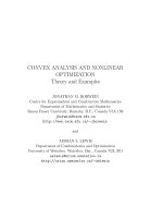
We can now analyze the impact of ABB as a frequency-tuning
mechanism at each V
DD
point. Notice that the relative-tuning range is not
the same for all V
DD
values. In particular, we measured frequency spans of
approximately –87% to +188% at V
DD
=0.6V and approximately ±20% at
V
DD
=1.2V with respect to their nominal frequencies. The larger tuning
range of ABB at reduced supply voltages can be explained by the fact that
the threshold voltage is a larger portion of the gate drive of the transistors.
At such low gate drive, the frequency becomes very sensitive to changes in
V
th
. Notice that a tuning range of –87% at V
DD
=0.6V implies an 8.1× lower
frequency for RBB. In fact, at V

DD
=0.6V, the circuit operates in the
subthreshold region for strong reverse body-biasing conditions. In this
case, the current is exponentially related to the gate drive voltage, and the
frequency is much lower than in case of nominal body biasing. For the
measured silicon, ABB gives an absolute tuning range of 135MHz for the
chosen N-well and P-well voltages when operating at V
DD
=1.2V. At
V
DD
=0.6V, this tuning range is around 45MHz. Figure 2.6a shows a
contour plot of the ABB-scaling operation at V
DD
=1.2V. The contours are
at 20MHz intervals, and the nominal frequency is at 327MHz. Notice that
that the V
th
is about 0.43V on average for this technology at nominal V
DD
.
When operating at reduced V
DD
, the V
th
increases due to of drain-induced
barrier lowering (DIBL). At V
DD
=0.6V, the V
th

increases by about 100mV.
The large frequency reduction with AVS is because the supply voltage
becomes close to the V
th
. For those low V
DD
s, the transistors are no longer
velocity saturated (α=2). For the applied range, AVS renders an
approximate 20× frequency reduction. If the lower bound of AVS would
be set to 0.7V, the frequency reduces by about 7×.
Figure 2.6 Frequency dependence on body-bias voltages; (a) Independent well
biasing and V
DD
=1.2V, (b) Symmetrical well biasing and various V
DD
voltages.
Chapter 2 Technological Boundaries of Voltage and Frequency Scaling 33
it is possible to change the V
th
of the PMOS and NMOS transistors
independently and still attain the same frequency. Obviously, the choice of
V
th
has a significant impact on leakage power consumption as we will
show later in this chapter. Figure 2.6b shows the frequency tuning for the
ABB-scaling operation as function of a symmetrical well bias (V
nwell
=V
DD
–

V
pwell
) and various supply voltages. Notice that the frequency saturates for
strong, reverse body biasing due to its limited V
th
control range.
The same analysis has been performed for ringos in 90nm CMOS. A
summary of the measured frequency-scaling and tuning ranges is given in
Table 2.2. Notice the large frequency-scaling range for 65nm LP-CMOS
as well as the large frequency-tuning range at reduced V
DD
. For severe
reverse body biasing, the threshold voltage saturates yielding as a result an
asymptotic limit on the lowest possible operating frequency. Observe that
GP-CMOS shows a lower dependence on V
DD
and V
th
as compared to LP-
CMOS primarily because the threshold voltage of the former technology is
lower.
Table 2.2 Frequency-scaling and tuning ranges for 90nm/65nm CMOS.

90nm GP 90nm LP 65nm LP
AVS
3.4× 5.9× 20.1×
ABB
V
DD
/2

V
DD

[–29,24]%
[–8,6]%
[–81,76]%
[–27,15]%
[–87,188]%
[–22,19]%
AVS+ABB
5.1× 34.9× 194.1×
2.4 Power and Frequency Tuning
The ultimate use of the AVS and ABB schemes is for performance tuning
with performance being the optimal combination of frequency and power,
i.e. the lowest power for a given frequency. To investigate the available
power–frequency-tuning range offered by AVS and ABB in 65nm LP-
CMOS, we consider the same ring oscillator as before. Figure 2.7 presents
a plot of the ringo frequency as function of the total power of the CGU,
e.g. both CGU-static and dynamic power consumption of the ringo. In our
experiments, static power takes into account all sources of leakage, e.g.
subthreshold leakage, gate-oxide leakage, etc.

34 Maurice Meijer, José Pineda de Gyvez
000E+0
50E+6
100E+6
150E+6
200E+6
250E+6
300E+6

350E+6
400E+6
450E+6
000E+0 20E-6 40E-6 60E-6 80E-6 100E-6 120E-6 140E-6 160E-6 180E-6
Power consumption [W]
Frequency [Hz]
ABB
V
DD
=1.2V
V
DD
=1.1V
V
DD
=1.0V
V
DD
=0.9V
0.8V
0.7V
0.6V
maxV
th
minV
th
nomV
th
AVS

Figure 2.7 Frequency versus total power.
The plot of Figure 2.7 allows us to evaluate power savings and tuning-
range control of AVS and ABB. Measurement results indicate 82× power
savings by 20.1× frequency downscaling, using AVS when downscaling
V
DD
from 1.2V to 0.6V. The use of ABB at V
DD
= 1.2V results in ±22%
power and ±20% frequency tuning with respect to the nominal operating
point. At V
DD
= 0.6V, we observe a power-tuning range that spans from
78% to +217% and a frequency-tuning range from –87% to +188% with
respect to no ABB. The combination of AVS and ABB yields ~790×
power savings with ~194× frequency scaling from the highest possible
frequency (minimum V
th
) to the lowest one (maximum V
th
). These results
show the strength of the combined use of AVS and ABB.

250E+6
300E+6
350E+6
400E+6
450E+6
500E+6
550E+6

600E+6
500.0E-6 700.0E-6 900.0E-6 1.1E-3 1.3E-3 1.5E-3
Frequency [Hz]
V
DD
=1.2V
V
DD
=1.1V
V
DD
=1.0V
A
B
150E+6
200E+6
250E+6
300E+6
350E+6
400E+6
40E-6 60E-6 80E-6 100E-6 120E-6 140E-6 160E-6 180E-
6

V
DD
=1.2V
V
DD
=1.1V
V

DD
=1.0V
A
B
Frequency [Hz]
Frequency [Hz]
Power consumption [W]
Power consumption [W]

Figure 2.8 Frequency versus total power trade-off; (a) 65nm LP-CMOS, (b) 90nm
LP-CMOS.
Let us now explore possible power-performance tradeoffs by using AVS
and ABB. Figure 2.8a shows a zoom-in of Figure 2.7 at V
DD
=1.2V. If
AVS and ABB are applied such that the nominal V
DD
becomes 1.1V
Chapter 2 Technological Boundaries of Voltage and Frequency Scaling 35
instead of 1.2V, and the V
th
s are pulled to a smaller value as indicated by
arrow A in Figure 2.8a, we see that it is possible to achieve ~14% power
savings with no frequency penalty. A more aggressive V
DD
downscaling to
1.0V, while pulling the V
th
s to their minimum value, results in 40% power
savings at about 16% frequency penalty as indicated by arrow B. Similar

results have been found for 90nm LP-CMOS as shown in Figure 2.8b. In
this case, the index factors are 16% power savings with no frequency
penalty at V
DD
=1.1V and 39% power savings with 11% frequency penalty
at V
DD
=1.0V. The benefits of combined AVS+ABB are not found to be
technology-node dependent for the considered LP-CMOS process
technologies. For 90nm GP-CMOS, however, a slightly larger voltage
dependency of performance was observed. Downscaling from its nominal
V
DD
of 1.0V–0.9V, and lowering the V
th
s a minimum, results in ~23%
power savings with ~6% frequency penalty. At V
DD
=0.8V and minimum
V
th
s, ~48% power savings are achieved with ~18% frequency penalty only.
This indicates that there exists a lower frequency-tuning range with ABB
for GP-CMOS.
000E+0
20E-3
40E-3
60E-3
80E-3
100E-3

120E-3
-1.2 -1 -0.8 -0.6 -0.4 -0.2 0 0.2 0.4
P-well bias volta
g
e
[
V
]
Total power core [W]
N-well
biasing
V
DD
=1.2V
maxV
th
minV
th

Figure 2.9 Power of 90nm LP-CMOS core as a function of well biasing.
Next we will investigate the properties of ABB in 90nm LP-CMOS on
the shift register. Figure 2.9 shows the core’s total power for a given
circuit activity and V
DD
=1.2V. Each dot in the clouds is associated to an N-
well biasing condition. The line joining the clouds indicates the case when
symmetric well biasing is applied. Observe that the well biasing allows a
total power-tuning range of about 36mW; this represents about 40% of the
nominal power consumption.
36 Maurice Meijer, José Pineda de Gyvez

000E+0
20E-3
40E-3
60E-3
80E-3
100E-3
120E-3
000.0E+0 200.0E-6 400.0E-6 600.0E-6 800.0E-6 1.0E-3 1.2E-3 1.4E-3
Total power ringo [W]
Total power core [W]
V
DD
=1.2V
V
DD
=
0.6V
V
DD
=
0.7V
V
DD
=
0.8V
V
DD
=0.9V
V
DD

=1.0V
V
DD
=1.1V
ABB
AVS

Figure 2.10 Total power correlation for the shift register and the ringo for
different V
DD
values.
Figure 2.10 shows the power consumption correlation between the shift
register and the ringo for different V
DD
values. In this plot, we have used
the same conventions as before, i.e. each cloud is associated to a unique
V
DD
value and each point in the cloud corresponds to a unique N-well and
P-well bias combination. The shift register operates at the same V
DD
as the
CGU, while its operating frequency is provided by the CGU. The circuit
activity of the shift register is kept constant. The dynamic power
dominates the total power in both circuit blocks, and therefore, their total
power can be estimated by P ≈ aC
⋅
V
DD
2

⋅
f, where aC represents the
switching circuit capacitance. Since both circuit blocks operate at the same
supply voltage and frequency, their power consumption is linearly related
by a ratio determined by the switching circuit capacitance. This can be
observed in Figure 2.10, where the power consumption of the circuit
blocks remains linearly correlated while applying AVS and/or ABB.
Table 2.3 puts into perspective the power–frequency ranges for the
ringos in the considered process technologies. Notice that there exist large
power–frequency ranges for each process technology. For the cases of
AVS only, or AVS+ABB, the ratio of power and frequency shows a factor
of 4× energy savings when scaling for the nominal V
DD
to half of its value.
This indicates that the total ringo power is dominated by dynamic power
consumption. Furthermore, observe that LP-CMOS offers a larger power-
and frequency-tuning range than GP-CMOS when utilizing ABB alone.
The frequency-tuning range of GP-CMOS is about 3× lower.

Chapter 2 Technological Boundaries of Voltage and Frequency Scaling 37
Table 2.3 Power–frequency-tuning ranges for 90nm and 65nm CMOS.
90nm GP 90nm LP 65nm LP
AVS
Power savings +
frequency penalty
13.7×
3.4×
23.6×
5.9×
82.0×

20.1×
ABB
V
DD
/2
Power tuning
Frequency tuning
[–29,29]%
[–29,24]%
[–77,65]%
[–81,76]%
[–78,217]%
[–87,188]%
V
DD

Power tuning
Frequency tuning
[–9,10]%
[–8,6]%
[–25,14]%
[–27,15]%
[–25,28]%
[–22,19]%
AVS+ABB
Power savings +
frequency penalty
21.2×
5.1×
117.1×

34.9×
790.5×
194.1×
2.5 Leakage Power Control
Leakage power is one of the main concerns in deep submicron
technologies. In fact, AVS and ABB are often used for leakage reduction
purposes. For older process technologies, leakage current is dominated by
subthreshold conduction. Subthreshold leakage for a given device strongly
depends on threshold voltage choice, process condition, supply voltage,
and temperature. For sub-100nm CMOS, other leakage components have
become increasingly important [13]. The most prominent ones are direct
tunneling currents through the thin gate-oxide and gate-induced drain
leakage (GIDL). Both leakage components are strongly V
DD
dependent.
Figure 2.11 puts into perspective leakage current as a function of power
supply and temperature for a high-V
th
NMOS device in 65nm LP-CMOS
technology. These results are obtained through circuit simulations for a
typical process condition. Observe in Figure 2.11a that subthreshold
leakage, gate-oxide tunneling, and GIDL currents are of the same order of
magnitude at nominal process–voltage–temperature conditions. Both
Figure 2.11a,b show that the dominant leakage component in the total
leakage depends on the operating condition.
10E-15
100E-15
1E-12
10E-12
100E-12

0.4 0.5 0.6 0.7 0.8 0.9 1 1.1 1.2 1.3 1.4
Power supply voltage in [V]
Leakage current in [A/
μ
m]
Total leakage Subthreshold Gate oxide tunneling GIDL

10E-15
100E-15
1E-12
10E-12
100E-12
1E-9
-50 -25 0 25 50 75 100 125 150
Temperature in [degC]
Leakage current in [A
/
μ
m]
Total leakage Subthreshold Gate oxide tunneling GIDL

Figure 2.11 Leakage current trends for a 65nm LP-CMOS high-V
th
NMOS
device; (a) V
DD
dependency at 25°C, (b) temperature dependency at V
DD
=1.2V.
38 Maurice Meijer, José Pineda de Gyvez

Figure 2.12 shows the impact of AVS and ABB on the leakage current
for our CGU in 65nm LP-CMOS at 25°C. The plot shows measured
leakage current versus body bias for three distinct values of power supply.
Body biasing is applied symmetrically for N-well and P-well, respectively.
The forward and reverse body-biasing ranges are indicated. Clearly, it is
shown in Figure 2.12 that the leakage current grows exponentially when
applying forward body biasing; this is because of the increased
subthreshold leakage when lowering the V
th
s. In reverse body-biasing
operation, the leakage current achieves a minimum value around 500mV
RBB. For stronger reverse body biasing, GIDL dominates the leakage
current eliminating the ability of ABB to reduce leakage. Observe in
Figure 2.12 that applying RBB of 300mV at V
DD
=1.2V is as effective as
lowering V
DD
by that same amount. For larger RBB at V
DD
=1.2V, AVS
becomes more effective to reduce leakage. This is because GIDL and gate-
oxide leakage are strongly reduced for lower V
DD
operation.

1E-09
1E-08
1E-07
1E-06

-1.4 -1.2 -1 -0.8 -0.6 -0.4 -0.2 0 0.2 0.4 0.6
Well bias voltage [V]
CGU leakage current [A]
RBB
FBB
V
DD
=1.2V
V
DD
=0.9V
V
DD
=0.6V

Figure 2.12 Leakage reduction in 65nm LP-CMOS using AVS and ABB.
For the measured die sample, leakage reduces by 5.1× when V
DD
is
scaled down from 1.2V to 0.6V. When using ABB alone at V
DD
= 1.2V,
leakage decreases only by 2.9×. This low impact of ABB is because of a
high level of GIDL as explained before. When using ABB alone at
V
DD
=0.6V, leakage decreases by 6.8×. The combination of AVS with ABB
renders a leakage reduction of 34.6×. Forward body biasing by 0.4V at
V
DD

=1.2V, 0.9V, or 0.6V increases the leakage current by 7.4×, 10.2×, or
13.7×, respectively.
The actual leakage savings utilizing AVS and ABB are impacted by
temperature. At elevated temperatures, the V
th
s become lower causing
subthreshold leakage to become a bigger part of the total leakage current.
Chapter 2 Technological Boundaries of Voltage and Frequency Scaling 39
GIDL depends only weakly on temperature, and gate-oxide leakage is not
temperature dependent. We have also measured temperature dependence
of leakage current for various die samples to quantify its impact on the
potential of AVS and ABB, to reduce leakage. Figure 2.13 shows
experimental results for leakage reduction versus temperature for the same
die sample as before. Observe that AVS becomes less effective to reduce
leakage with increasing temperature, since the related leakage increase is
supply voltage independent. However, the leakage increase is threshold
voltage dependent, and therefore, ABB can reduce leakage slightly more
effectively when temperature increases. At very high temperatures, i.e. the
case of 100°C, the V
th
is lowered so much that ABB cannot further reduce
leakage because of the constrained ABB range we used in our
experiments. The trend of AVS+ABB shows the collective effect of
reducing leakage by AVS and ABB. In this case, leakage savings are about
constant for temperatures up to 75°C.

9.7
34.6
35.8
30.8

5.1
4.0
3.2
2.4
2.8
3.5
3.5
2.6
6.8
8.9
7.2
17.4
0
10
20
30
40
25 50 75 100
Temperature [degC]
Leakage reduction factor
AVS ABB (Vdd=1.2V) ABB (Vdd=0.6V) AVS+ABB

Figure 2.13 Temperature-dependent leakage reduction in 65nm LP-CMOS.
The actual leakage savings achieved by AVS and ABB are also
impacted by process parameter variations. Subthreshold leakage strongly
depends on process state, while gate-oxide leakage and GIDL are only
weakly dependent. Leakage current of the CGU has been measured for 40
die samples from the same silicon wafer at 25°C. We have observed a
leakage current ranging from 17.3nA to 322.6nA, depending on the die
sample. This corresponds to leakage current variations of about 18.7×.

40 Maurice Meijer, José Pineda de Gyvez
Table 2.4 shows the average leakage current savings for 65nm LP-
CMOS obtained for the measured 40 die samples. The reduction factors
for 90nm GP- and LP-CMOS technologies are also shown in this Table.
The product of leakage savings with AVS (V
DD
/2) and ABB yields
substantial benefits as indicated in row AVS+ABB.
Table 2.4 Leakage current reduction for 90nm and 65nm CMOS at 25°C operation.

90nm GP 90nm LP 65nm LP
AVS
5.3× 3.3× 5.6×
ABB
V
DD
/2
V
DD

4.1×
1.2×
6.6×
3.5×
4.5×
2.5×
AVS+ABB

21.6× 21.5× 24.8×
2.6 Performance Compensation
Understanding the trade-offs in performance and power is not sufficient to
ensure a successful outcome of the IC. The basic problem is that failure of
deep submicron process technologies to continue with constant process
tolerances opens avenues for new challenging low-power process options
and emerging design technologies. Basically, the assimilation of distinct
high-performance, low operating power, and low standby power devices
requires circuits and systems that concurrently exploit many degrees of
freedom in both fabrication and design technologies.

130nm CMOS
90nm CMOS
65nm CMOS
Towards slow-corner
Towards fast-corner

Figure 2.14 Energy spread across various technology nodes.
Figure 2.14 shows the impact of process variability on performance
spread of a single inverter for various technology nodes. A proportional
inverter sizing was done across technology nodes for comparison
Chapter 2 Technological Boundaries of Voltage and Frequency Scaling 41
purposes. The inverter has further a fan-out of four gates. The vertical axis
basically shows the spread of speed over three process corners, e.g.
typical–slow–fast. The horizontal axis shows the normalized energy per
operation. Notice that the performance window spread for 130nm, 90nm,
and 65nm CMOS is about 40%, 50%, and 70%, with respect to the
nominal operating conditions, respectively. What this graph also shows is
that for a constant throughput, the wider the performance spread, the better
the opportunities for energy savings are if voltage scaling is applied. For

instance, in 65nm CMOS, the normalized speed of “1” can be achieved at
an energy of “0.6” instead of at an energy of “1” if the power supply is
scaled down. Today’s design practices advocate a worst-case design style
to ensure a target speed. This brings as implications overhead in area and
power as shown in Figure 2.14. Basically, a worst-case design requires
stronger cells, which are bigger in area and are also bigger power
consumers, to meet timing closure of designs that fall beyond the 3σ due
to process variability.
Figure 2.15 shows the impact of process variability on leakage power of
the same inverter. One can see that leakage power spread at nominal supply
voltage can span over 7×, 9×, and 11× for 130nm, 90nm, and 65nm CMOS,
respectively. This spread can be detrimental in ultra low-power designs.
90nm CMOS
65nm CMOS
130nm CMOS
Towards slow-corner
Towards fast-corner

Figure 2.15 Leakage spread across various technology nodes.
As the variation of fundamental parameters such as channel length,
threshold voltage, thin oxide thickness, and interconnect dimensions goes
well beyond acceptable limits, “on-the-fly” performance compensation is
becoming necessary. The influence of process parameter spread on circuit
42 Maurice Meijer, José Pineda de Gyvez
behavior becomes higher and higher. For instance, in older technologies
greater than 0.18μm, a V
th
spread of say 50mV on a nominal V
th
of 450mV

was not that crucial; in nanometer technologies with a nominal V
th
of
250mV, this variation can make circuit operation quite difficult.

250E+6
275E+6
300E+6
325E+6
350E+6
375E+6
400E+6
425E+6
450E+6
000E+0 50E-9 100E-9 150E-9 200E-9 250E-9 300E-9 350E-9 400E-9 450E-9
CGU leaka
g
e current
[
A
]
Frequency [Hz]
slow
fast
typical
unbalanced
Corner results
fast
427MHz, 430nA
fnsp

337MHz, 144nA
typical
336MHz, 71nA
snfp
335MHz, 88nA
slow
270MHz, 17nA

Figure 2.16 Frequency and leakage spread for 40 die samples of the same 65nm
LP-CMOS wafer.
Figure 2.16 shows an example of frequency and leakage spread in which
ringo frequency versus CGU leakage current is plotted at nominal V
DD
for
40 die samples coming from the same 65nm LP-CMOS wafer. The five
corner specifications for ringo frequency versus CGU leakage, as
determined from circuit simulations, are also indicated in Figure 2.16. The
total frequency and the leakage spread of the measured die samples are
about 100MHz and 305nA, respectively. This translates into a relative
frequency spread of ~36% and a relative leakage spread of ~18.7×. Note
that we consider the samples with frequencies below “typical” as yield
losses, while samples above “typical” are consuming unnecessary extra
power. Moreover, the leakage current for a “fast” corner sample is about
~6.1× higher as compared to the “typical” reference, while the leakage
current for a “slow” corner sample is about ~4.2× lower.
Next, we will discuss three strategies for compensating the undesired
process-dependent frequency and leakage spread by means of post-silicon
tuning. A first strategy is to perform post-silicon tuning with ABB only.
From experiments, we have determined the tuning ranges for “fast” and
“slow” samples. Figure 2.17 shows the potential of ABB to compensate

performance for the same die samples as shown before. A 21% frequency
increment from the slow corner renders a target frequency of 327MHz, and