Báo cáo hóa học: " Research Article On the Problem of Bandwidth Partitioning in FDD Block-Fading Single-User MISO/SIMO Systems" docx

Hindawi Publishing Corporation
EURASIP Journal on Advances in Signal Processing
Volume 2008, Article ID 735929, 13 pages
doi:10.1155/2008/735929
Research Article
On the Problem of Bandwidth Partitioning in FDD
Block-Fading Single-User MISO/SIMO Systems
Michel T. Ivrla
ˇ
c and Josef A. Nossek
Lehrstuhl f
¨
ur Netzwerktheorie und Signalverarbeitung, Technische Universit
¨
at M
¨
unchen, 80290 M
¨
unchen, Germany
Correspondence should be addressed to Michel T. Ivrla
ˇ
c,
Received 6 November 2007; Revised 2 April 2008; Accepted 26 June 2008
Recommended by Sven Erik Nordholm
We report on our research activity on the problem of how to optimally partition the available bandwidth of frequency division
duplex, multi-input single-output communication systems, into subbands for the uplink, the downlink, and the feedback. In the
downlink, the transmitter applies coherent beamforming based on quantized channel information which is obtained by feedback
from the receiver. As feedback takes away resources from the uplink, which could otherwise be used to transfer payload data,
it is highly desirable to reserve the “right” amount of uplink resources for the feedback. Under the assumption of random
vector quantization, and a frequency flat, independent and identically distributed block-fading channel, we derive closed-form
expressions for both the feedback quantization and bandwidth partitioning which jointly maximize the sum of the average payload

data rates of the downlink and the uplink. While we do introduce some approximations to facilitate mathematical tractability, the
analytical solution is asymptotically exact as the number of antennas approaches infinity, while for systems with few antennas,
it turns out to be a fairly accurate approximation. In this way, the obtained results are meaningful for practical communication
systems, which usually can only employ a few antennas.
Copyright © 2008 M. T. Ivrla
ˇ
c and J. A. Nossek. This is an open access article distributed under the Creative Commons Attribution
License, which permits unrestricted use, distribution, and reproduction in any medium, provided the original work is properly
cited.
1. INTRODUCTION
In this work, we consider a single-user, frequency division
duplex (FDD) wireless communication system which can be
modeled as a frequency flat fading multi-input single-output
(MISO) system in the downlink, and as a frequency flat fading
single-input multi-output (SIMO) system in the uplink.In
order to achieve the maximum possible channel capacity of
such a communication system, perfect knowledge about the
normalized channel vector has to be present at the receiver in
the uplink, and at the transmitter in the downlink.
In the uplink, the channel between the single transmit
and the multiple receive antennas (the SIMO case) can
be estimated by the receiver by evaluating a received pilot
sequence prior to applying coherent receive beamforming
based on the estimated channel vector, so-called maximum
ratio combining [1]. In the downlink, the situation is more
complicated. Because of the frequency gap between the
uplink and the downlink band, the channel which was
estimated by the receiver in the uplink cannot be used by
the transmitter in the downlink. The channel between the
multiple transmit antennas and the single receive antenna

(the MISO case) has to be estimated by the receiver, and
then transferred back in a quantized form to the transmitter,
suchthatcoherenttransmitbeamformingcanbeapplied,so-
called maximum ratio transmission [2].
The more bits are used for the quantized feedback, the
higher is the obtainable beamforming gain, and hence, the
downlink throughput. However, feedback is taking away
resources from the uplink, which could otherwise be used
to transfer payload data. It is highly desirable to reserve
the “correct” amount of uplink resources for the feedback
such that the overall performance of the downlink and the
uplink is maximized. Moreover, the division of the available
bandwidth into the uplink band and the downlink band
should also be optimized. In this report, we will propose
a way on obtaining an optimized partition of the total
bandwidth into subbands for the uplink, the downlink, and
the feedback.
1.1. Related work
Coherent transmit beamforming for MISO systems based on
quantized feedback was proposed in [3]. The beamforming
2 EURASIP Journal on Advances in Signal Processing
vector is thereby chosen from a finite set, the so-called
codebook, that is known to both the transmitter and the
receiver. After having estimated the channel, the receiver
chooses that vector from the codebook which maximizes
signal-to-noise ratio (SNR). The index of the chosen vector
is then fed back to the transmitter. There are different
ways of designing codebooks for vector quantization [4].
By extending the work in [5], a design method for orthog-
onal codebooks is proposed in [6] which can achieve

full transmit diversity order using quantized equal gain
transmission. In [7], nonorthogonal codebooks are designed
based on Grassmannian line packing [8]. Analytical results
for the performance of optimally quantized beamformers
are developed in [9], where a universal lower bound on
the outage probability for any finite set of beamformers
with quantized feedback is derived. The authors of [10]
propose to maximize the mean-squared weighted inner
product between the channel vector and the quantized
vector, which is shown to lead to a closed form design
algorithm that produces codebooks which reportedly behave
well also for correlated channel vectors. Nondeterminis-
tic approaches using so-called random vector quantiza-
tion (RVQ) are proposed in [11–13], where a codebook
composed of vectors which are uniformly distributed on
the unit sphere is randomly generated each time there
is a significant change of the channel. It is shown in
[11] that RVQ is optimal in terms of capacity in the
large system limit in which both the number of transmit
antennas and the bandwidth tend to infinity with a fixed
ratio. For low number of antennas, numerical results [14]
indicate that RVQ still continues to perform reasonably
well.
The important aspect that feedback occupies resources
that could otherwise be used for payload data, is investigated
in [15, 16]. The cost for channel estimation and feedback is
taken into account in [15] by scaling the mutual information
that is used as a vehicle to compute the block fading
outage probability. In [16], the optimum number of pilot
bits and feedback bits in relation to the size of a radio

frame is analyzed. In particular, for an i.i.d. block fading
channel, upper and lower bounds on the channel capacity
with random vector quantization and limited-rate feedback
are derived, which are functions of the number of pilot
symbols and feedback bits. The optimal amount of pilot
symbols and feedback bits as a fraction of the size of the
radio frame is derived under the assumption of a constant
transmit power and large number of transmit antennas. (It
is shown in [16] that for a constant transmit power, as
the size of the radio frame approaches infinity forming a
fixed ratio with the number N of transmit antennas, the
optimal pilot size and the optimum number of feedback
bits normalized to the antenna number tend to zero at
rate(log N)
−1
.)
1.2. Our approach: optimum resource sharing
While [15, 16] do consider that feedback and pilot symbols
occupy system resources, they treat the flow of payload data
as unidirectional, namely, flowing in the downlink from
the multiantenna transmitter to the single-antenna receiver
(the MISO-case). Furthermore, the asymptotic analysis in
[16] for large antenna numbers keeps the transmit power
constant, which leads to a receiver SNR that increases with
the number of transmit antennas.
In our approach, we propose to share the totally available
resources between downlink, uplink, and feedback such that
the overall system performance in terms of the sum of the
throughputs of the downlink and the uplink is maximized.
In this way, we can also maintain a given and finite SNR at

the receivers with lowest amount of transmit power. Keeping
the receiver SNR constant, instead of the transmit power, has
the advantage that any desired trade-off between bandwidth
efficiency and transmit power efficiency can be implemented
[17]. (We will see in Section 4.7 that a receive SNR of
about 6 dB is optimum in the sense that it maximizes
the product of bandwidth efficiency and transmit power
efficiency.) To be more specific, we are interested in the
following situation.
(1) We consider an FDD system which has N transmit
antennas and a single receive antenna in the down-
link, and N receive antennas and a single transmit
antenna in the uplink.
(2) The system has available a total usable bandwidth B.
(The term “usable” refers to the fact that the com-
munication system may need additional bandwidth
resources, e.g., for channel estimation, synchroniza-
tion, traffic control channels, and guard bands. The
total “usable” bandwidth is the bandwidth which
the system has available for transporting downlink
payload data, uplink payload data, and feedback
information.)
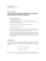
(3) The bandwidth B has to be partitioned into a
bandwidth B
DL
for the downlink band, and into a
bandwidth B
UL
for the uplink band. Furthermore, a
part of the uplink band, with bandwidth B

FB
,hasto
be reserved for feedback rather than for carrying the
uplink payload data. This bandwidth partitioning is
shown in Figure 1.
(4) The uplink and the downlink bands are separated
by a frequency gap, such that instantaneous channel
state information obtained from the uplink cannot
be used in the downlink, hence making feedback of
instantaneous channel state information necessary.
Notice that such a gap in frequency between the
uplink band and the downlink band is necessary in
any FDD system due to implementation issues. (The
huge imbalance in receive and transmit power (usu-
ally more than 100 dB) at the basestation necessitates
a significant gap in frequency in order to insure that
the order of the required filters does not become too
large to be implementable.)
(5) Both the uplink band and the downlink band can be
modeled as frequency flat fading.
M. T. Ivrla
ˇ
c and J. A. Nossek 3
(6) The proposed bandwidth partitioning takes place
according to

B
opt
UL
, B

opt
DL
, B
opt
FB

=
arg max
(B
UL
,B
DL
,B
FB
)

R
DL
(B
DL
, B
FB
)+R
UL
(B
UL
, B
FB
)


,
such that
⎧
⎪
⎪
⎪
⎪
⎪
⎪
⎪
⎨
⎪
⎪
⎪
⎪
⎪
⎪
⎪
⎩
B
DL
> 0,
B
UL
> 0,
0 <B
FB
≤ B
UL
,

B
UL
+ B
DL
= B,
R
UL
= μR
DL
,
(1)
where
R
DL
and R
UL
denote the average payload data
rates in the downlink and the uplink, respectively,
and μ
≥ 0 is a symmetry factor which accounts for
different requirements on payload data rate in the
two different directions. For μ
= 0, the communi-
cation becomes unidirectional (downlink only), that
is, the whole uplink band can be used for feedback.
Of course, (1) can be restated as maximization of
R
DL
with the same constraints, since R
UL

is kept in a fixed
ratio with
R
DL
. However, the formulation (1)hasa
convenient structure which can be used to arrive at
an elegant solution.
1.3. Major assumptions
In order to solve (1), we make the following assumptions.
(1) In the downlink, the N transmit antennas are used
for maximum ratio transmission based on quantized
channel feedback.
(2) An i.i.d. frequency-flat block-fading channel is
assumed for the uplink and the downlink. That is,
the channel is assumed to remain constant within
the time T
dec
, and then to abruptly change to a new,
independent realization.
(3) The channel coefficients between any receive and
transmit antenna are uncorrelated.
(4) Channel estimation errors at the receivers are negli-
gible.
(5) The bandwidth B is completely usable for payload
and feedback. There are additional resources needed
for channel estimation, however, those have to be
present with or without the feedback scheme, so
we do not consider those resources as part of the
optimization.
(6) The quantization of the normalized channel vector

is performed by RVQ using b bits per antenna.
The codebook, therefore, consists of 2
Nb
(pseudo)-
random vectors which are chosen uniformly from
the unit sphere. Each time the channel changes, a
new realization of the codebook is generated. In this
way, the performance of the RVQ is averaged over all
random codebooks (uniform on the unit sphere).
B
B
UL
B
DL
B
FB
FB UL-data DL-data
Figure 1: Partitioning of the available bandwidth into a downlink
band and an uplink band, where the latter accommodates also a
band reserved for feedback. Note that the gap in frequency between
the uplink and the downlink band is not shown in this figure.
(7) The quantized feedback bits are protected by capacity
approaching error control coding.
(8) Capacity approaching error control coding is also
used for the payload data both in the uplink and the
downlink.
(9) The feedback bits can be decoded correctly with
negligible outage.
(10) Feedback has to be received within the time T,where
T

 T
dec
.
2. GENERIC SOLUTION
From the assumptions in Section 1.3,wecanwritewiththe
help of the newly introduced parameter η (which is used
as a nice mathematical way to obtain the notion of outage
capacity while, in effect, only ergodic capacity has to be
computed):
N
·b
T
= η·B
FB
·E[log
2
(1 + SNR
UL
)], (2)
since Nb bits of feedback have to be reliably transferred
within T seconds, requiring an information rate of Nb/T
bits per second. It is important to note that the instanta-
neous receive SNR in the uplink (SNR
UL
) and hence, the
instantaneous uplink channel capacity, fluctuates randomly
because of the block fading channel. Nevertheless, it is highly
important that the feedback information can be decoded
correctly in most cases. In order to ensure correct decoding
with a given probability, we include the factor η,with0<

η
≤ 1. Therefore, in (2), we equate the information rate
Nb/T with η times the ergodic uplink channel capacity.
The smaller the value of η, the higher is the probability
that the instantaneous channel capacity is above η times its
mean value, and hence, the smaller is the probability of a
channel outage. For instance, with N
= 4 and i.i.d. Rayleigh
fading with an average uplink SNR of 6 dB, it turns out,
that correct decoding is possible with 99% probability when
we set η
= 0.4. Therefore, assuming these parameters, (2)
equates the feedback information rate Nb/T, with the 1%-
outage capacity of the feedback channel. In the following, we
consider η as a given system parameter. Note that for large
number of antennas, the fluctuation of SNR
UL
around its
mean value becomes small. Hence, η can be chosen close to
unity:
lim
N →∞
η = 1. (3)
4 EURASIP Journal on Advances in Signal Processing
Furthermore,
R
UL
(b) = B
UL
·E[log

2
(1 + SNR
UL
)]
  
R
UL
without feedback
−
Nb
Tη
,(4)
and finally,
R
DL
(b) = B
DL
·E[log
2
(1 + SNR
DL
)], (5)
where SNR
DL
is the receive SNR in the downlink. Since the
obtainable beamforming gain depends on the quantization
resolution,
R
DL
is a function of the number b of feedback bits

per antenna. The original optimization problem (1)cannow
be solved in three steps.
(1) Assuming that we know B
opt
DL
, find the optimum quan-
tization resolution.
b
opt

B
opt
DL

=
arg max
b

R
DL
(b)+R
UL
(b)

,
= arg max
b

B
opt

DL
·E[log
2
(1 + SNR
DL
)] −
Nb
Tη

,
(6)
since SNR
UL
does not depend on b. Note that this b
opt
will
depend on B
opt
DL
, whose value is unknown at this moment,
but will be computed in the following step.
(2) Find the optimum bandwidth partition.
From (2) immediately follows that
B
opt
FB

B
opt
DL


=
N·b
opt

B
opt
DL

η·T·E[log
2
(1 + SNR
UL
)]
. (7)
Using the last constraint in (1), it follows from (4)and(5)
that
B
opt
UL

B
opt
DL

=
μ
E[log
2
(1 + SNR

DL
)]
E[log
2
(1 + SNR
UL
)]
B
opt
DL

B
opt
DL


 
≥0
+ B
opt
FB

B
opt
DL

.
(8)
With the second to last constraint in (1), it follows from (8)
that

B
opt
DL
=
B − B
opt
FB

B
opt
DL

1+μ(E[log
2
(1 + SNR
DL
)]/E[log
2
(1 + SNR
UL
)])
.
(9)
Note that (9)isanimplicit solution, since it contains the
desired B
opt
DL
both on its left-hand side and on its right-hand
side. However, we will see in Section 4.5 that (9)canbe
transformed into an explicit form, where B

opt
DL
is given as an
explicit function of known system parameters.
(3) Obey the remaining constraints.
As long as
b
opt
> 0,
B
opt
FB
<B,
(10)
we can see from (7)–(9) that the remaining first three con-
straints of (1) are fulfilled. As a consequence, (10)is
necessary and sufficient for the existence of the solution.
The original constraint optimization problem (1)is,
therefore, essentially reduced to the unconstrained problem
(6) of finding b
opt
.
2.1. Simplifications
For the sake of mathematical tractability, we will use the
approximation:
E[log
2
(1 + SNR
DL
)] ≈ log

2
(1 + E[SNR
DL
]). (11)
Note that
E[log
2
(1 + SNR
DL
)] −→ log
2
(1 + E[SNR
DL
])
for

SNR
DL
−→ 0,
N
−→ ∞ .
(12)
That is, the approximation (11) becomes an almost exact
equality either in the low SNR regime, or for large number
of antennas. The latter is due to the fact that with increasing
N the diversity order increases, such that the SNR varies less
and less around its mean value. Using this approximation in
(6), we obtain the optimization problem:

b

opt
= arg max
b
⎛
⎜
⎝
B
DL
·log
2
⎛
⎜
⎝
1+E[SNR
DL
]
  
function of b
⎞
⎟
⎠
−
Nb
Tη
⎞
⎟
⎠
,
(13)
whichismucheasiertosolvethan(6). Because of (12), it

follows that

b
opt
−→ b
opt
for

SNR
DL
−→ 0,
N
−→ ∞ .
(14)
2.2. Preview of key results
In the following sections, we present a detailed derivation
of the solution to the problem (13) and the associated
optimum bandwidth partitioning problem in closed form.
More precisely, for a given system bandwidth B and a
symmetry factor μ, we obtain analytical expressions for
the optimum quantization resolution and the optimum
bandwidth that should be allocated for the downlink, the
uplink, and the feedback.
While the solution is asymptotically exact as the number
of antennas approaches infinity, we will see that it is also
fairly accurate for low antenna numbers. In this way, the
obtained solution is not only attractive from a theoretical
point of view, but also applicable for practical communica-
tion systems. For instance, in the process of standardization
of future wireless communication systems, the proposed

solution may provide valuable input for the discussion about
how fine to quantize channel information and how much
resources to reserve for its feedback.
In order to gain a better feeling about what can be
done with the solution developed in this manuscript, we
would like to present some of the obtained results. For
the sake of clarity, let us look at a concrete example
system, where a totally usable bandwidth B has to be
partitioned. Let the time T during which the feedback
has to arrive be given by T
= 100/B. The considered
system should be a symmetrical one, where the average
M. T. Ivrla
ˇ
c and J. A. Nossek 5
payload data rates are the same in uplink and downlink
(symmetry factor μ
= 1). Moreover, let us assume that
the encoded feedback can be decoded correctly with high
probability, say 99%. This can be accomplished by setting the
factor η (see (2) and the discussion in Section 2)properly.
(The actual value for the factor η depends on the fading
distribution in the uplink, which also depends on the
number N of receive antennas. In the case of i.i.d. Rayleigh
fading it turns out that η
= (0.175, 0.4, 0.57,0.7, 0.79, 1)
in conjunction with N
= (2, 4, 8, 16,32,∞) guarantees
decoding errors below 1%.) In both the uplink and the
downlink, the average SNR is set to 6 dB, which is the

optimum value for a single-stream system that attempts
to be both bandwidth-efficient and power-efficient at the
same time (see the discussion in Section 4.7 for more
details). Using the results derived in this manuscript, we
obtain the optimum bandwidth partition for the described
example system for different number of antennas N
∈
{
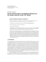
2, 4, 8, 16,32,∞}, as shown in Figure 2. Note that starting
from about 5.4% of the total bandwidth for N
= 2
antennas, the optimum amount of feedback bandwidth
increases strictly monotonic with increasing antenna num-
ber, reaching almost 10% for N
= 8. In case that N →∞,
itturnsoutthatitisoptimumtoreserveexactly20%of
the totally available bandwidth for feedback. It is interesting
to note that this last asymptotic result essentially only
depends on the symmetry factor μ,butnot on system
parameters like bandwidth B,ortimeT. By setting the
symmetry factor μ
= 0, we obtain a pure downlink
system, which makes use of the whole uplink band for
feedback. As we will see in Section 4.6,thissystemismost
happy with a feedback bandwidth of exactly 1/3 of the
available bandwidth, as the number of antennas approaches
infinity.
3. RANDOM VECTOR QUANTIZATION
As described in Section 2, the optimum bandwidth par-
titioning problem can essentially be reformulated in the

unconstrained optimization problem (13). As a prerequisite
for its solution, we need to know the functional relation-
ship:
b
−→ E[SNR
DL
], (15)
that is, in what way the average SNR in the downlink
is influenced by the resolution with which the channel
information is quantized. In this section, the function (15)is
derived, assuming random vector quantization (RVQ). The
motivation for RVQ is both mathematical tractability [13],
and the fact that it can indeed be optimal for large number
of antennas [11].
3.1. Transmit b eamforming
In the downlink, the frequency flat i.i.d. block fading channel
between the N transmit antennas and the single receive
antenna is described by the channel vector h
∈ C
N×1
.The
transmitter applies beamforming with a beamforming vector
u
∈ C
N×1
such that the signal,
r
=

P

T
u
2
2
·E[|s|
2
]
·h
T
u·s + ν, (16)
is received, in case that the signal s
∈ C is transmitted with
power P
T
. Herein, the term ν ∈ C denotes receiver noise
with power σ
2
ν
. The receive SNR in the downlink, therefore,
becomes
SNR
DL
=
E[|r −ν|
2
|h, u]
E[|ν|
2
]
,

=
P
T
·h
2
2
σ
2
ν
  
SNR
max
DL
·
|
h
T
u|
2
h
2
2
·u
2
2
  
γ
,
(17)
where SNR

max
DL
is the maximum obtainable downlink SNR,
while 0
≤ γ ≤ 1 is the relative SNR, which is maximum for
coherent beamforming, that is, if u
= const·h
∗
.
3.2. Quantization and feedback procedure
The receiver generates quantized feedback in the following
way.
(1) The channel vector h is estimated (with negligible
error).
(2) A sequence of 2
Nb
i.i.d. pseudorandom vectors
(u
1
, u
2
, , u
2
Nb
) is generated such that
u
i
∝ N
C
(0

N
, I
N
). (18)
(3) The transmitter generates the same sequence of
pseudorandom vectors.
(4) In case that u
i
is chosen as the beamforming vector,
the resulting relative SNR will be
γ
i
=
|
h
T
u
i
|
2
h
2
2
·u
i

2
2
. (19)
(5) The vector u

i
∗
is selected as the beamforming vector
according to
i
∗
= arg max
i∈{1,2, ,2
Nb
}
γ
i
. (20)
(6) The Nb bit long binary representation of the index
i
∗
is protected by capacity approaching error control
coding and fed back to the transmitter.
(7) Upon successful decoding of the encoded feedback
data, the transmitter begins to use the beamforming
vector u
i
∗
, which leads to an SNR:
SNR
DL
= SNR
max
DL
·γ

i
∗
. (21)
6 EURASIP Journal on Advances in Signal Processing
1B0.8B0.6B0.4B0.2B0
f
N
= 2
N = 4
N
= 8
N
= 16
N
= 32
N
→∞
FB UL-data DL-data
Figure 2: Optimum partitioning of the available bandwidth for a
symmetric (μ
= 1) system operating at average SNR of 6 dB with a
bandwidth-time product of BT
= 100.
3.3. Average receive SNR in the downlink
The average receive SNR in the downlink can now be written
as [13]
E[SNR
DL
] =
P

T
σ
2
ν
·E

h
2
2
·E[γ
i
∗
|h]

,
=
P
T
σ
2
ν
·E

h
2
2


 
SNR

max
DL
·

1 −2
Nb
·B

2
Nb
,
N
N −1

,
= SNR
max
DL
·

1 −2
Nb
·B

2
Nb
,
N
N −1


,
(22)
where
SNR
max
DL
denotes the maximum possible average
SNR that is obtainable in the downlink, and B(
·, ·)is
the beta function [18, 19]. Notice that b
→∞ implies
E[SNR
DL
] → SNR
max
DL
, while b = 0 implies E[SNR
DL
] =
SNR
max
DL
/N.
3.4. Simplifications
While (22)providesanexact expression for the average SNR
in the downlink, it does not seem particularly attractive
to use it directly in the optimum quantization resolution
problem given in (14) since b appears both outside and inside
the beta function. We propose to apply some approximation
to (22) in order to facilitate the solution of the optimum

bandwidth partitioning problem. From [16, 20], an upper
and lower bound on E[γ
i
∗
|h]forb>0canbegiven:
1
≤
E[γ
i
∗
|h]
1 −2
−b
≤ 1+Ψ(b, N), (23)
where
Ψ(b, N)
=
1+(C
Γ
−1)2
−b
+2
−Nb
(1 −2
−b
)(N −1)
, (24)
and C
Γ
= 0.577216 is the Euler Gamma constant [18, 19].

A consequence of
lim
N →∞
Ψ(b, N) = 0 (25)
is that for a constant number b>0 of bits per antenna, the
upper and lower bounds in (23) converge towards each other,
hence,
E[γ
i
∗
|h]−→1−2
−b
for N −→ ∞, b=positive constant.
(26)
The situation is more complicated in case that b approaches
zero as N approaches
∞. Note that b should never approach
zero more quickly than 1/N because, otherwise, the total
number of feedback bits per time T would drop below
unity, which we may consider pathological for a system that
attempts to use feedback. For b
= β/N,withβ ≥ 1 being a
constant, we find
lim
N →∞
Ψ

β
N
, N


=
C
Γ
+2
−β
β·log
e
2
< 1.56. (27)
For large β,weobtainfrom(27)
lim
β →∞
lim
N →∞
Ψ

β
N
, N

=
0. (28)
For β
≥ 84, the upper bound in (23) is less than 1% ahead of
the lower bound. In this way, we can use the approximation
(26) even when b goes linearly down with increasing N,
provided that the factor of proportionality β is large enough.
In practice, β
≥ 100 should be sufficient. We will now

make a final adjustment and propose to use the following
approximation:
E[γ
i
∗
|h] ≈ 1 −2
−b
N −1
N
≥
1
N
. (29)
This does not change the asymptotic behavior for large N,
but makes the approximation exact for b
= 0 since E[γ
i
∗
|h]
is lower bounded by 1/N. By substituting (29) into (22), we
finally arrive at the approximation which we will make use of
subsequently:
E[SNR
DL
] ≈ SNR
max
DL
·

1 −2

−b
N −1
N

. (30)
It is interesting to note that from (30),
(b
= 1) −→ E[SNR
DL
]
≈
lim
b →∞
E[SNR
DL
] + lim
b →0
E[SNR
DL
]
2
,
(31)
that is, for 1 bit quantization per antenna, one can already
achieve half of the maximum possible gain obtainable by the
feedback. For large number of transmit antennas, the loss
in performance compared to ideal coherent beamforming
approaches3dBfrombelow,whenb
= 1 quantization bit
per antenna is used.

M. T. Ivrla
ˇ
c and J. A. Nossek 7
86420
b
0.5
0.6
0.7
0.8
0.9
1
E[γ
i
∗
]
N = 2
Exact
Approximation
(a)
6543210
b
0.2
0.4
0.6
0.8
1
E[γ
i
∗
]

N = 4
Exact
Approximation
(b)
32.521.510.50
b
0.2
0.4
0.6
0.8
1
E[γ
i
∗
]
N = 8
Exact
Approximation
(c)
1.510.50
b
0
0.1
0.3
0.5
0.7
E[γ
i
∗
]

N = 16
Exact
Approximation
(d)
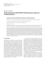
Figure 3: Comparison of the exact value of E[γ
i
∗
]from(22) and the approximation from (30).
Before we end this section, let us briefly have a look
at the difference between the approximation (30) and the
exact solution (22) for the average downlink SNR. We can
see in Figure 3 the average relative SNR, that is, E[γ
i
∗
]asa
function of the number b of quantization bits per antenna
number for different antenna numbers N. For small values
of b,particularlyforb
≤ 1, the approximation does a fairly
good job, even for very small (e.g., N
= 2) antenna numbers.
For larger values of b, the approximation requires higher
antenna numbers to be reasonably accurate. In practice,
N
≥ 8mightbesufficient. Note that in the limit N →∞,
the approximation becomes exact for constant b,andfor
b
= β/N, it becomes exact as also β →∞.Wewillmakeuseof
this property in the next section.
4. OPTIMUM BANDWIDTH PARTITIONING

The results of Section 3.4 on the obtainable average receive
SNR in the downlink for a given resolution of random
vector quantization will be used now to solve the bandwidth
partitioning problem. As our first task, we will compute
the optimum quantization resolution, which maximizes the
sum throughput of the uplink and the downlink. Second,
we show that the product B
DL
T has to be above a certain
threshold, such that feedback can be used in a beneficial
manner. We then proceed to a closed-form solution of the
optimum bandwidth partitioning problem. We elaborate on
the asymptotic behavior of large antenna numbers, where
we also discuss the special cases of symmetrical uplink and
8 EURASIP Journal on Advances in Signal Processing
downlink, and a pure downlink system (which uses the whole
uplink band for feedback). Finally, we treat the question
of optimum SNR and its relationship with the bandwidth
partitioning problem.
4.1. Quantization resolution
When we substitute (30) into (13), we find

b
opt
= arg max
b
B
DL
·log
2


1+SNR
max
DL
·

1 −2
−b
N −1
N

−
Nb
Tη

.
(32)
Because the second derivative of the cost function in (32)is
negative for N>1andallb>0, the optimization problem
(32) has a unique solution. It can easily be found by solving
for the root of the first partial derivative of the cost function
with respect to b,forwhichwefind

b
opt
= log
2


1+

B
DL
Tη
N

·
N −1
N
·
SNR
max
DL
1+SNR
max
DL

. (33)
In order to make this expression better suited to our problem,
let us express
SNR
max
DL
in terms of the actual average downlink
SNR that is present for a quantization resolution of b
=

b
opt
.
Using our approximation from (30), we have

SNR
DL
= SNR
max
DL
·

1 −2
−

b
opt
N −1
N

, (34)
where
SNR
DL
is the average SNR in the downlink that we
obtain in the optimum b
=

b
opt
. By substituting (33) into
(34), we obtain—after small rearrangements—the following
relationship:
SNR
DL

=
SNR
max
DL
(B
DL
Tη/N) − 1
1+(B
DL
Tη/N)
, (35)
which we can also write in its inverse form:
SNR
max
DL
= SNR
DL
+

1+SNR
DL

N
B
DL
Tη
. (36)
By substituting (36) into (33), we obtain for the optimum
quantization resolution


b
opt
= log
2

N −1
N

1+
B
DL
Tη
N
·
SNR
DL
1+SNR
DL

. (37)
The optimum feedback information rate can be written as
R
opt
FB
=
N·

b
opt
T

. (38)
Example 1. The following parameters, B
DL
= 20 kHz, T =
50 ms, N = 4, and η = 0.4,yieldanoptimumresolutionof

b
opt
≈ 5.93 for SNR
DL
= 4. This translates into a feedback
information rate of about 474 bps, which is a fraction of
1086420
RVQ resolution b per antenna (bits)
15
20
25
30
35
40
45
50
Cost function (kbps)
Approximate cost-function
Exact cost-function
+150%
4.93 bits
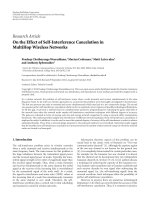
5.93 bits
Figure 4: Comparison of the exact cost function (no approxi-
mations used) from (6), and the approximate cost function from

(32). The former is computed numerically. The average SNR in the
optimal points (star-shaped markers) is set to
SNR
DL
= 4inboth
cases.
about 1.0% of the downlink throughput. (More precisely,
this is the fraction of the feedback rate with respect to the
downlink throughput of the average channel. Because the
latter is an upper bound for the true average throughput, the
ratio is (slightly) larger. For i.i.d. Rayleigh distributed fading,
the exact ratio turns out to be about 1.07%.)
4.2. Accuracy of the analytical solution
In obtaining the analytical solution (37) for the optimum
resolution of the RVQ, we have made use of the two approxi-
mations from (11), and (30). While the approximation error
can be made arbitrarily small by increasing the number of
antennas, there remains, of course, an approximation error
for finite—especially low—number of antennas. In order
to check how much the proposed solution in (37)deviates
from the exact one (which has to be computed numerically),
we analyze the example scenario from above. We use the
parameters: B
DL
= 20 kHz, T = 50 ms, N = 4, η = 0.4,
and
SNR
DL
= 4, when measured at the optimal value of b.
Additionally, we assume i.i.d. Rayleigh fading, in which case

we obtain the results displayed in Figure 4.Twocurvesare
shown there as functions of the resolution b per antenna of
the RVQ. The top-most curve corresponds to the cost func-
tion from (32) which incorporates the two approximations
in (11)and(30). The lower curve shows the cost function
from (6), where we use no approximations. The latter is
computed numerically. The star-shaped markers indicate
the optimum resolutions. As can be seen from Figure 4,
the analytical solution from (37) slightly overestimates the
true optimum resolution (in this case 5.93 bits, instead
of 4.93 bits). However, since the maximum of both cost
functions is rather flat for values of b which are larger than
the respective optimum value, the results obtained from (37)
represent a conservative approximation of the true optimum
M. T. Ivrla
ˇ
c and J. A. Nossek 9
resolution. From careful observation of the two curves shown
in Figure 4, it turns out that the exact cost function, evaluated
at the resolution b
= 5.93 bits, has dropped by less than
0.2% compared to its maximum value. We conclude that the
proposed solution (37) is usable in practice even for as low
number of antennas as N
= 4.
4.3. Minimum required bandwidth-time product
The solution (37) is valid if and only if

b
opt

> 0. This sets a
lower limit on the product B
DL
T:
B
DL
T>
1
η
·
1+SNR
DL
SNR
DL
·
N
N −1
. (39)
Because the feedback has to arrive (much) earlier than the
assumed i.i.d. block fading channel changes its realization,
that is, T
 T
dec
has to hold, it follows with (39) that
B
DL
T
dec

1

η
·
1+SNR
DL
SNR
DL
·
N
N −1
. (40)
4.4. Feedback rate for large systems
When we substitute (37) into (38), and multiply both sides
by T,weobtain
R
opt
FB
T = log
2


1 −
1
N

N

+log
2



1+
α
N

N

, (41)
where
α
= B
DL
Tη
SNR
DL
1+SNR
DL
. (42)
Using lim
t →∞
(1 + x/t)
t
= e
x
, and lim
N →∞
η = 1, it follows
that
lim
N →∞
R

opt
FB
=
α −1
T log
e
2




η=1
,
(43)
= log
2
(e)·

B
DL
SNR
DL
1+SNR
DL
−
1
T

.
(44)

Since R
opt
FB
is increasing with N, it follows that
R
opt
FB
<B
DL
log
2
e. (45)
The optimum feedback rate remains finite, even for arbitrary
large number of antennas or average SNR. With (38), it
follows from (44) that

b
opt
−→
β
N
,asN
−→ ∞ , (46)
where
β
= log
2
(e)·

B

DL
T
SNR
DL
1+SNR
DL
−1

. (47)
Recall from Section 3.4 that the approximation (30) that was
used to arrive at the solution (37)requiresβ to have a large
value, like β>100. In practice, this usually represents no
problem, since at reasonably large
SNR
DL
,saySNR
DL
= 4,
already a relatively small bandwidth-time product of B
DL
T =
88 will guarantee β>100. For large β, the term 1/T becomes
negligible in (44), so that it follows that
lim
β →∞

lim
N →∞
R
opt

FB

=
B
DL
SNR
DL
1+SNR
DL
log
2
(e). (48)
Because in the limit β
→∞and N →∞the used approxi-
mations (11)and(30) become exact, the result (48)holds
exactly.
4.5. Bandwidth partitioning
Recall from Section 2 that the bandwidth partitioning prob-
lem (1) is essentially solved once we know the optimum
quantization resolution. By substituting (37) into (7), and
applying the approximation (12) also for the uplink, we find
that the bandwidth which is optimum to reserve for feedback
is given by
B
opt
FB
=
N
Tη
·

log
2

(N −1)/N

1+(B
DL
Tη/N)·

SNR
DL
/

1+SNR
DL

log
2

1+SNR
UL

,
(49)
where
SNR
UL
is the average SNR in the uplink.
Example 2. For the case N
= 4, SNR

DL
= SNR
DL
= 4, T =
50 ms, B
DL
= 20 kHz, and η = 0.4, we find from (49) that
B
opt
FB
≈ 511 Hz, or about 2.56% of the downlink bandwidth.
It is somewhat impractical that the optimum feedback
bandwidth according to (49)isexpressedasafunctionof
the downlink bandwidth B
DL
instead of the totally available
bandwidth B. This problem will, however, be solved in a
moment. When we substitute (49) into (9), we obtain
B
opt
DL
·

1+μ
log
2

1+SNR
DL


log
2

1+SNR
UL


=
B−
N
Tη
·
log
2

(N −1)/N

1+

B
opt
DL
Tη/N

·

SNR
DL
/


1+SNR
DL

log
2

1+SNR
UL

.
(50)
Note that B
opt
DL
appears both on the left- and the right-hand
side of (50). However, it is shown in the appendix that (50)
can be solved explicitly for B
opt
DL
:
B
opt
DL
=
N
Tη
·
1+SNR
DL
SNR

DL
·

W

(NΦ/(N −1))

1+ SNR
UL

Φ+BTη/N
log
e

1+ SNR
UL

Φlog
e

1+ SNR
UL

−
1

,
(51)
10 EURASIP Journal on Advances in Signal Processing
where W(·) is the Lambert W-function [21, 22], and

Φ
def
=
1+SNR
DL
SNR
DL
·

1+μ
log
2

1+SNR
DL

log
2

1+SNR
UL


. (52)
Now that we know B
opt
DL
explicitly as a function of the total
bandwidth B, and the remaining system parameters, we can
compute B

opt
UL
immediately as
B
opt
UL
= B −B
opt
DL
, (53)
while B
opt
FB
can be computed from (49) by substituting B
DL
by
B
opt
DL
from (51):
B
opt
FB
=
N
Tη
·
log
e


(N−1)·W

NΦ/(N−1)

Z
Φ+BTη/N
log
e
Z

/

NΦlog
e
Z

log
e
Z
,
(54)
where Z denotes

1+SNR
UL

.
The Lambert W function has to be computed numeri-
cally. A simple but accurate approximation is given in [23]as
follows:

W(x)
≈
⎧
⎪
⎪
⎪
⎪
⎪
⎪
⎪
⎪
⎨
⎪
⎪
⎪
⎪
⎪
⎪
⎪
⎪
⎩
0.665·(1 + 0.0195 log
e
(1 + x))·log
e
(1 + x)+0.04
for 0
≤ x ≤ 500,
log
e

(x − 4) −

1 −
1
log
e
x

·
log
e
(log
e
(x))
for x>500.
(55)
For x>500, the relative error of (55)isbelow3.3
×10
−4
.
Example 3. Let B
= 20 kHz, T = 50 ms, N = 4, SNR
DL
=
4, SNR
UL
= 3, η = 0.4, and the symmetry factor μ = 1/2.
Evaluation of (51), (53), and (54) leads to the following
optimum bandwidth partition: B
opt

DL
≈ 12.32 kHz, B
opt
UL
≈
7.677 kHz, and finally B
opt
FB
≈ 523.7 Hz. Therefore, the
resources reserved for feedback consume about 6.8% of
the uplink band, which equals about 2.6% of the total
bandwidth. With (37)and(38), we can compute that the
optimum RVQ should be performed with a resolution of

b
opt
≈ 5.24 bits per antenna. In total, this amounts to about
21 bits. That means that the optimum RVQ codebook con-
sists of some 2 million, four-dimensional, complex vectors.
(If the codebook is precomputed and stored, it would require
around 128 MB of memory. If it is generated on the fly, its
generation would require about half a second computing
time on a high-performance workstation at the time of
writing. This shows that for the given example scenario,
random vector quantization may not be easy-to-implement.)
The optimum feedback rate equals R
opt
FB
≈ 419 bps, while
the payload throughputs in down and uplink compute to

R
DL
≈ 28.6kbps and R
UL
≈ 14.3kbps, respectively. As a
consequence, the feedback rate amounts to almost 1% of
the sum-throughput of uplink and downlink, which equals
42.9 kbps. This is the highest possible sum-throughput that
can be achieved with the given system parameters.
4.6. Bandwidth partitioning for large systems
Recall that the approximations (12)and(30)becomeexact
as N
→∞ and β →∞. Let us, therefore, have a look at the
results for large systems, that is, systems with large number
of antennas, and large bandwidth. The latter is necessary to
assure that β asgivenin(47) is also large. By substituting (48)
into (7), we obtain by noting that lim
N →∞
η = 1 that
(N,BT)
−→ ∞ :
B
opt
FB
B
DL
=
SNR
DL


1+SNR
DL

·
log
e

1+SNR
UL

.
(56)
In the following, we will restrict the discussion to the
important special case of
SNR
UL
= SNR
DL
def
= SNR, (57)
from which we have
(N,BT)
−→ ∞ :
B
opt
FB
B
DL
=
SNR


1+SNR

·log
e

1+SNR

.
(58)
Note that
0 <B
opt
FB
<B
DL
, (59)
while
B
opt
FB
−→
⎧
⎨
⎩
0forSNR −→ ∞ ,
B
DL
for SNR −→ 0.
(60)

In this way, the optimum amount of bandwidth that has
to be reserved for feedback can be varied widely with the
average SNR. While for very large SNR, this extra bandwidth
becomes very small, it can raise to the size of the downlink
bandwidth in case that the SNR is very small. So, what
SNR
should we choose? It is tempting to define the “optimum”
SNR such that the bandwidth for feedback is neither too
small nor too large, say, half-way between its minimum
and maximum value. Therefore, SNR
opt
has to fulfill the
following equation:
SNR
opt

1+SNR
opt

·
log
e

1+SNR
opt

=
1
2
, (61)

from which
SNR
opt
can be computed numerically:
SNR
opt
≈ 3.92, (62)
which equals approximately to 6 dB. We will see in
Section 4.7 that
SNR
opt
also maximizes the product of
bandwidth efficiency and transmit power efficiency, which
further motivates to call this
SNR the “optimum” SNR. In the
M. T. Ivrla
ˇ
c and J. A. Nossek 11
following, we assume SNR = SNR
opt
.From(58), it follows
that
B
opt
FB
=
1
2
·B
DL

. (63)
By substituting (63) into (9), and solving for B
DL
,wecan
write for the optimum downlink bandwidth the following
simple expression:
(N,BT)
−→ ∞ :
B
opt
DL
B
=
2
3+2μ
. (64)
Recall that the parameter μ is the given ratio between the
average throughput in the uplink and the average throughput
in the downlink. Since B
DL
+ B
UL
= B, we can obtain also for
the optimum uplink bandwidth a simple expression:
(N,BT)
−→ ∞ :
B
opt
UL
B

=
1+2μ
3+2μ
. (65)
Finally, it follows from (63)and(64) that
(N,BT)
−→ ∞ :
B
opt
FB
B
=
1
3+2μ
. (66)
Notice that for a pure downlink system, we have
μ
= 0 −→

B
opt
FB
: B
opt
DL
: B
opt
UL

=

(1 : 2 : 1), (67)
that is, one third of the bandwidth is used for feedback,
which occupies the whole uplink band, while the remaining
bandwidth is used for the downlink. On the other hand, in a
symme trical system, we have
μ
= 1 −→

B
opt
FB
: B
opt
DL
: B
opt
UL

= (1 : 2 : 3), (68)
that is, one fifth of the total bandwidth is reserved for
feedback, which occupies one third of the uplink band, while
the remaining bandwidth is equally split for payload in up-
and downlink.
4.7. Optimum signal to noise ratio
Let us now have a second look at the “optimum” average
SNRasitisimplicitlydefinedin(61). Using the relationship
between transmit power P
T
and SNR:
SNR

= α·
P
T
BN
0
, (69)
where N
0
is the noise power density, and α>0 is a constant
channel gain, the channel capacity of an additive white
Gaussian noise (AWGN) channel is given by
C(B, P
T
) = B log
2

1+α·
P
T
BN
0

. (70)
The bandwidth and transmit power efficiency [17]are
defined as
η
B
def
=
C(B, P

T
)
B
= log
2
(1 + SNR),
(71)
η
P
def
=
C(B, P
T
)
max
B
C(B, P
T
)
=
log
e
(1 + SNR)
SNR
.
(72)
In this way, the bandwidth efficiency quantifies how many
bits of information can be transferred per second in the given
bandwidth, while the transmit power efficiency tells how
much channel capacity is obtained for the given transmit

power compared to what could be achieved at most with this
transmit power. The equality in (72)followsfrom
max
B
C(B, P
T
) = lim
B →∞
C(B, P
T
),
= α·
P
T
N
0
log
2
e,
= B·SNR·log
2
(e).
(73)
Because η
B
increases with SNR, while η
P
decreases with
SNR, the system becomes less power efficient, when its
bandwidth efficiency increases, and vice versa. Therefore,

each given SNR corresponds to a specific trade-off between
these two fundamental efficiencies. Since both efficiencies
are important, the optimum SNR can be defined as the one
which maximizes the product of bandwidth and transmit
power efficiency:
SNR
opt
= arg max
SNR
(log
e
(1 + SNR))
2
log
e
(2)·SNR
. (74)
By solving for the root of the derivative with respect to SNR,
we find that
SNR
opt
(1 + SNR
opt
) ·log
e
(1 + SNR
opt
)
=
1

2
(75)
must hold. Comparing (75)with(61), we can see that
the SNR which maximizes the product of bandwidth and
transmit power efficiency is the same
SNR which was
defined optimum on the grounds of feedback bandwidth in
Section 4.6.
5. SUMMARY, CONCLUSION, AND OUTLOOK
5.1. Summary
An in-depth derivation of an asymptotically exact, analytical
solution of the problem of optimum feedback quantization
and partitioning of bandwidth in FDD-MISO/SIMO com-
munication systems was presented in this report. While we
had to introduce some approximations to facilitate math-
ematical tractability, the analytical solution is nevertheless
asymptotically exact as the number of antennas approaches
infinity. Furthermore, it turns out to be a fairly accurate
approximation even for systems with only a few antennas.
5.2. Conclusion
From the results we may conclude the following:
(1) The decision on the resolution of channel quan-
tization and the amount of resources reserved for
feedback should be based on the ground of a suitable
optimization problem rather than done by heuristic
ad hoc methods, as it possibly might have been the
case in the standardization of past and current mobile
communication systems.
12 EURASIP Journal on Advances in Signal Processing
(2) The merits of feedback systems should always be

weighted against the loss of resources that the
feedback occupies.
(3) Too less feedback can be more harmful than too
much. For instance, we can observe from Figure 4
that for the example system, a resolution of about
5 bits per antenna is optimum. However, increasing
the number of bits to, say 10, is much less harmful
than decreasing the amount to 2 bits per antenna.
(4) In the large-system limit, the amount of feedback
is pretty large, for instance, 1/3 of the available
bandwidth in a pure downlink system.
(5) Using quantized channel feedback can boost the
performance compared to a baseline system which
uses no feedback, as can be observed from Figure 4.
5.3. Outlook
The presented results have a number of limitations and
short-comings. In the following, there is a list—as brief,
incomplete, and subjective as it may be—of further direc-
tions worthy to explore by the research community in the
future.
(1) The assumption of the i.i.d. block-fading channel
should be given up for a more realistic, correlated
block-fading channel model. This has direct impact
on the quantization, since the correlations allow for
predictive quantization.
(2) While the presented results can easily be generalized
to some special multiuser scenarios (like round-robin
TDMA), substantial further work is required to cover
multiuser systems with channel-aware scheduling.
(3) Consider space division multiplexing (SDM) and

space division multiple access (SDMA).
APPENDIX
DERIVATION OF EQUATION (51)
For ease of notation, let us write (50) in the following way:
aB
opt
DL
+ blog
e

c + dB
opt
DL

+ e = 0, (A.1)
where
a
= 1+μ
log
2

1+SNR
DL

log
2

1+SNR
UL


,(A.2)
b
=
N
Tηlog
e

1+SNR
UL

,
(A.3)
c
=
N −1
N
,
(A.4)
d
=
N −1
N
·
Tη
N
·
SNR
DL
1+SNR
DL

,
(A.5)
e
=−B.
(A.6)
With the substitution
B
opt
DL
=
1
d

exp

−
x −
ed −ac
bd

−
c

,(A.7)
we can write (A.1)as
x
·exp(x) =
a
bd
·exp

ac
−ed
bd
. (A.8)
By denoting with W(
·) the Lambert W-function [21, 22],
which is defined by its inverse
W
−1
(x) = x·exp(x), (A.9)
it follows from (A.8) that
x
= W

a
bd
·exp

ac −ed
bd

. (A.10)
When we substitute (A.10) into (A.7), we obtain
B
opt
DL
=
1
d


exp

−
W

a
bd
exp(
−A)

−
A

−
c

, (A.11)
wherewehaveintroduced
A
=
ed −ac
bd
, (A.12)
for ease of notation. By defining
y
=−W

a
bd
exp(

−A)

, (A.13)
it follows with (A.9) that
A
=−log
e

−
bd
a
y
·exp(−y)

. (A.14)
When we substitute (A.13)and(A.14) into (A.11), we obtain
B
opt
DL
=
b
a
W

a
bd
exp(
−A)

−

c
d
, (A.15)
while from (A.12), and (A.2)–(A.6) it follows that
A
=−log
e

1+SNR
UL

·

BTη
N
+
1+
SNR
DL
SNR
DL

1+μ
log
2

1+SNR
DL

log

2

1+SNR
UL


.
(A.16)
With
Φ
def
=
1+SNR
DL
SNR
DL
·

1+μ
log
2

1+SNR
DL

log
2

1+SNR
UL



, (A.17)
we can write
a
bd
exp(
−A) =
NΦ
N −1

1+SNR
UL

Φ+BTη/N
log
e

1+SNR
UL

.
(A.18)
Substituting (A.18) into (A.15), we finally arrive with (A.2)–
(A.5) at the explicit formula for the optimum downlink
bandwidth given in (51).
M. T. Ivrla
ˇ
c and J. A. Nossek 13
ACKNOWLEDGMENT

The authors wish to express their sincere thanks to the
anonymous reviewers for their effort and comments which
ultimately helped in improving the paper.
REFERENCES
[1] W. C. Jakes Jr., Mobile Microwave Communication,JohnWiley
& Sons, New York, NY, USA, 1974.
[2] T. K. Y. Lo, “Maximum ratio transmission,” IEEE Transactions
on Communications, vol. 47, no. 10, pp. 1458–1461, 1999.
[3] A. Narula, M. J. Lopez, M. D. Trott, and G. W. Wornell,
“Efficient use of side information in multiple-antenna data
transmission over fading channels,” IEEE Journal on Selected
Areas in Communications, vol. 16, no. 8, pp. 1423–1436, 1998.
[4] R. M. Gray and D. L. Neuhoff, “Quantization,” IEEE Trans-
actions on Information Theory, vol. 44, no. 6, pp. 2325–2383,
1998.
[5] R. W. Heath Jr. and A. Paulraj, “A simple scheme for transmit
diversity using partial channel feedback,” in Proceedings of the
32nd Asilomar Conference on Signals, Systems & Computers
(ACSSC ’98), vol. 2, pp. 1073–1078, Pacific Grove, Calif, USA,
November 1998.
[6]D.J.LoveandR.W.HeathJr.,“Equalgaintransmission
in multiple-input multiple-output wireless systems,” IEEE
Transactions on Communications, vol. 51, no. 7, pp. 1102–
1110, 2003.
[7] D. J. Love, R. W. Heath Jr., and T. Strohmer, “Grassmannian
beamforming for multiple-input multiple-output wireless
systems,” IEEE Transactions on Information Theory, vol. 49, no.
10, pp. 2735–2747, 2003.
[8] J. H. Conway, R. H. Hardin, and N. J. A. Sloane, “Packing lines,
planes, etc.: packings in Grassmannian spaces,” Experimental

Mathematics, vol. 5, no. 2, pp. 138–159, 1996.
[9] K. K. Mukkavilli, A. Sabharwal, E. Erkip, and B. Aazhang, “On
beamforming with finite rate feedback in multiple-antenna
systems,” IEEE Transactions on Information Theory, vol. 49, no.
10, pp. 2562–2579, 2003.
[10] J. C. Roh and B. D. Rao, “Transmit beamforming in multiple-
antenna systems with finite rate feedback: a VQ-based
approach,” IEEE Transactions on Information Theory, vol. 52,
no. 3, pp. 1101–1112, 2006.
[11] W. Santipach and M. L. Honig, “Asymptotic capacity of beam-
forming with limited feedback,” in Proceedings of the IEEE
International Symposium on Information Theory (ISIT ’04),p.
290, Chicago, Ill, USA, June-July 2004.
[12] W. Santipach and M. L. Honig, “Signature optimization
for CDMA with limited feedback,” IEEE Transactions on
Information Theory, vol. 51, no. 10, pp. 3475–3492, 2005.
[13] C. K. Au-Yeung and D. J. Love, “On the performance of ran-
dom vector quantization limited feedback beamforming in a
MISO system,” IEEE Transactions on Wireless Communications,
vol. 6, no. 2, pp. 458–462, 2007.
[14] D. J. Love, R. W. Heath Jr., W. Santipach, and M. L. Honig,
“What is the value of limited feedback for MIMO channels?”
IEEE Communications Magazine, vol. 42, no. 10, pp. 54–59,
2004.
[15] S. Bhashyam, A. Sabharwal, and B. Aazhang, “Feedback
gain in multiple antenna systems,” IEEE Transactions on
Communications, vol. 50, no. 5, pp. 785–798, 2002.
[16] W. Santipach and M. L. Honig, “Capacity of beamforming
with limited training and feedback,” in Proceedings of the IEEE
International Sy m posium on Information Theory (ISIT ’06),pp.

376–380, Seattle, Wash, USA, July 2006.
[17] M. T. Ivrla
ˇ
c, Wireless MIMO Systems: Models, Performance,
Optimization, Shaker, Aachen, Germany, 2005.
[18] I. N. Bronstein, K. A. Semendjajew, G. Musiol, and G. M
¨
uhlig,
Taschenbuch der Mathematik, Harri Deutsch, Thun, Germany,
1995.
[19] M. Abramowitz and I. A. Stegun, Handbook of Mathematical
Functions with Formulas, Graphs, and Mathematical Tables,
Dover, New York, NY, USA, 1972.
[20] D. Kershaw, “Some extensions of W. Gautschi’s inequalities for
the gamma function,” Mathematics of Computation, vol. 41,
no. 164, pp. 607–611, 1983.
[21] R. M. Corless, G. H. Gonnet, D. E. G. Hare, D. J. Jeffrey,
andD.E.Knuth,“OntheLambertWfunction,”Advances in
Computational Mathematics, vol. 5, no. 1, pp. 329–359, 1996.
[22] F. Chapeau-Blondeau and A. Monir, “Numerical evaluation
of the Lambert W function and application to generation
of generalized Gaussian noise with exponent 1/2,” IEEE
Transactions on Signal Processing, vol. 50, no. 9, pp. 2160–2165,
2002.
[23] A. Ringwald and F. Schrempp, “QCDINS 2.0—a Monte Carlo
generator for instanton-induced processes in deep-inelastic
scattering,” Computer Physics Communications, vol. 132, no. 3,
pp. 267–305, 2000.