Báo cáo hóa học: " Research Article Joint Effects of Synchronization Errors of OFDM Systems in Doubly-Selective Fading Channels Wen-Long Chin1 and Sau-Gee Chen (EURASIP Member)2" pptx

Hindawi Publishing Corporation
EURASIP Journal on Advances in Signal Processing
Volume 2008, Article ID 840237, 9 pages
doi:10.1155/2008/840237
Research Article
Joint Effects of Synchronization Errors of OFDM Systems in
Doubly-Selective Fading Channels
Wen-Long Chin
1
and Sau-Gee Chen (EURASIP Member)
2
1
Department of Engineering Science, National Cheng Kung University, Tainan 701, Taiwan
2
Department of Electronics Engineering and Institute of Electronics, National Chiao Tung University, Hsinchu 30050, Taiwan
Correspondence should be addressed to Wen-Long Chin,
Received 26 July 2008; Revised 8 November 2008; Accepted 3 December 2008
Recommended by George Tombras
The majority of existing analyses on synchronization errors consider only partial synchronization error factors. In contrast, this
work simultaneously analyzes joint effects of major synchronization errors, including the symbol time offset (STO), carrier
frequency offset (CFO), and sampling clock frequency offset (SCFO) of orthogonal frequency-division multiplexing (OFDM)
systems in doubly-selective fading channels. Those errors are generally coexisting so that the combined error will seriously degrade
the performance of an OFDM receiver by introducing intercarrier interference (ICI) and intersymbol interference (ISI). To assist
the design of OFDM receivers, we formulate the theoretical signal-to-interference-and-noise ratio (SINR) due to the combined
error effect. As such, by knowing the required SINR of a specific application, all combinations of allowable errors can be derived,
and cost-effective algorithms can be easily characterized. By doing so, it is unnecessary to run the time-consuming Monte Carlo
simulations, commonly adopted by many conventional designs of synchronization algorithms, in order to know those combined
error effects.
Copyright © 2008 W L. Chin and S G. Chen. This is an open access article distributed under the Creative Commons Attribution
License, which permits unrestricted use, distribution, and reproduction in any medium, provided the original work is properly
cited.

1. INTRODUCTION
Orthogonal frequency-division multiplexing (OFDM) is a
promising technology for broadband transmission due to its
high spectrum efficiency, and its robustness to the effects
of multipath fading channels and impulse noises. However,
OFDM systems are sensitive to synchronization errors.
There are three major synchronization errors, including
the symbol time offset (STO), carrier frequency offset (CFO),
and sampling clock frequency offset (SCFO) in OFDM
systems. When the symbol time (ST) is not located in the
intersymbol interference (ISI) free region, ISI is introduced.
The time-selective channel, CFO, and SCFO will introduce
additional intercarrier interference (ICI).
The effects of the synchronization errors had been
studied in literature, for example, in [1–15]. For conciseness,
we only discuss some representative works here. In [1],
the signal-to-interference-and-noise ratio (SINR) is analyzed
considering the effect of the CFO in time-selective channels;
the work in [2] analyzes the effect of the STO in frequency-
selective channels; the work in [3] also analyzes the effect
of the STO without considering ISI; the work in [4]
analyzes the effect of the Doppler spread; the work in [5]
analyzes the effect of the CFO and SCFO in time-selective
channels; the work in [6] only analyzes the effect of the
STO in doubly-selective channels; the works in [7–9]analyze
the synchronization errors separately in frequency-selective
channels; the works in [10–12] analyze the effect of the
CFO in frequency-selective channels; and the works in [13–
15] consider the combined effects of the STO and CFO in
frequency-selective channels.

Some works [1–6, 8–15] only consider partial synchro-
nization errors; some works [1–9, 12, 13, 15] separately
consider synchronization errors; and some works [2,
6–14]
only consider frequency-selective channels. In addition, the
works in [6, 8, 10, 11, 13, 14] consider the STO, while assum-
ing that the STO is small; therefore, nonnegligible ISI was
often neglected. In summary, the current analyses mostly do
not consider joint effects of the combined synchronization
errors due to nonideal synchronization process in the envi-
ronments of mobility (causing time-selective channel effect)
and nonline-of-sight (NLOS) (causing multipath channel
2 EURASIP Journal on Advances in Signal Processing
Table 1: Comparison of synchronization errors analyses.
Reference Consider ISI Consider STO Consider CFO Consider SCFO Fast fading channel Combined analysis
[1]NoNo Yes No Yes No
[2]YesYes No No No No
[3]NoNo No No Yes No
[4] No No Yes Yes Yes No
[5] Yes Yes No No Yes No
[6] No Yes Yes Yes No No
[7] Yes Yes Yes Yes No No
[8] No Yes Yes Yes No No
[9] No No Yes No No No
[10, 11] No Yes Yes No No Yes
[12] No No Yes No No No
[13] No Yes No No No No
[14] No Yes Yes No No Yes
[15] No No Yes No No No
T h i s w o r k Ye s Ye s Ye s Ye s Ye s Ye s

Data
source
Signal
mapper
X
l,k
N-point
IFFT
CP
insertion
P/S DAC
1/T
S
Data
sink
Signal
demap-
per
Equalizer

X
l,k
N-point
FFT
CP
removal
S/P
ADC
n
δ

1/T

S
= (1 + ε
t
)/T
S
e
−j2π(1−ε
f
) f
c
t
e
j2πf
c
t
AWG N
Channel
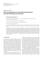
Figure 1: A simplified OFDM system model.
effect). For clarity, Ta b le 1 summarizes the concerned errors
and conditions, of some key representative works and the
proposed work, on the synchronization error analyses.
The main contribution of this paper is that for better
characterizations of synchronization errors under a practical
communication environment, that is, in doubly-selective
fading channels, we analyze joint effects of the mentioned
three major synchronization errors, without the assumption
of small STO. Another contribution is that compact forms
can be derived from our work to gain further insights on the

synchronization error effects. To this end, we first analyze
the signal model of the combined synchronization errors
in time-selective and frequency-selective fading channels by
extending the works in [1–15]. Next, based on this model,
the theoretical SINR is formulated. The derived SINR can
be exploited to obtain all possible combinations of syn-
chronization errors that meet the required SINR constraint,
knowing that the allowable synchronization errors could
help design suitable synchronization algorithms and shorten
the design cycle. To gain further insights, some compact
results are deduced from the derived SINR formulation. In
addition, the works in [1, 2] are found to be special cases
of this work; and our work is more accurate than that in
[10].
The rest of this paper is organized as follows. The
notations used in this work are summarized in the Notaions
section at the end of the paper. The OFDM system model in
doubly-selective fading channels is introduced in Section 2.
The signal model with synchronization errors is analyzed,
and its theoretical SINR is formulated in Section 3.Some
compact results are given in Section 4. Numerical and
simulation results are provided in Section 5. Finally, we
conclude our work in Section 6.
2. SYSTEM AND CHANNEL MODELS
2.1. System model
In the following discussion, all the quantities indexed with
l belong to the lth symbol. A simplified OFDM system
W L. Chin and S G. Chen 3
model is shown in Figure 1. In this figure, X
l,k

/

X
l,k
is
the transmitted/received frequency-domain data at the kth
subcarrier; n
δ
is the STO; 1/T
S
is the transmitter’s sampling
frequency; 1/T

S
= (1 + ε
t
)/T
S
is the receiver’s sampling
frequency, where ε
t
is the SCFO normalized by 1/T
S
; ε
f
is
the CFO normalized by the subcarrier spacing; and f
c
is
the carrier frequency. On the transmitter side, N complex

data symbols are modulated onto N subcarriers by using
the inverse fast Fourier transform (IFFT). The last N
G
IFFT
output samples are copied to form the CP which is inserted
at the beginning of each OFDM symbol. By inserting the CP,
a guard interval is created so that ISI can be avoided and
the orthogonality among subcarriers can be sustained. The
receiver uses the fast Fourier transform (FFT) to demodulate
received data.
2.2. Channel model
In this work, h
l
(n, τ) denotes the τth channel tap of the
discrete time-selective CIR at time n of the lth symbol.
Furthermore, the following two assumptions regarding the
channels are made: (a) the channels are wide-sense stationary
and uncorrelated scattering (WSSUS), and (b) the Doppler
spectrum follows Jakes’ model [16]. Based on these assump-
tions, the cross-correlation of the CIR can be obtained by
E

h
l

n
1
, τ
1


h
∗
l

n
2
, τ
2

=
E

h
l

n
1
, τ
1

h
∗
l

n
2
, τ
2

δ


τ
1
− τ
2

=
J
0

βΔ
n

σ
2
h
τ


τ=τ
1
=τ
2
,0≤ τ ≤ τ
d
,
(1)
where δ(
·) is the Dirac delta function; J
0

(·) is the zeroth-
order Bessel function of the first kind; Δ
n
 n
1
− n
2
; σ
2
h
τ
=
E[|h
l
(τ)|
2
] is the power of the τth channel tap; τ
d
is the
maximum delay spread of the channel; and β
= 2πf
d
T/N
where f
d
represents the maximum Doppler shift, f
d
T is the
normalized Doppler frequency (NDF), N is the number of
subcarriers, and T

= NT
S
is the symbol duration.
3. ANALYSIS OF RECEIVED FREQUENCY-DOMAIN
DATA AND SINR
For convenience, let us define the start of the lth symbol
(excluding the CP with length N
G
) at the time origin zero
in the time coordinate. The estimated ST can be found
to be located in one of the following three regions of an
OFDM symbol: the Bad-ST1 region, the Good-ST region
(also known as the ISI-free region), and the Bad-ST2 region
in which the STOs are confined within the ranges of
−N
G
≤
n
δ
≤−N
G
+ τ
d
−1, −N
G
+ τ
d
≤ n
δ
≤ 0, and 1 ≤ n

δ
≤ N −1,
respectively. Note that the first two regions are in the guard
interval. Moreover, the transmitted signal of the lth symbol
can be represented as
x
l
(t) =
1
N

m
X
l,m
e
j2πmt/NT
S
, −N
G
T
S
≤ t<NT
S
,(2)
where m is the transmitter subcarrier index. It is assumed
that the symbol index l is the same for both the receiver
and the transmitter sides due to the ST and/or SCFO
compensations. Consequently, after undergoing a multipath
fading channel, the received signal can be determined as
x

l
(t) =
τ
d

τ=0
x
l

t − τT
S

h
l
(t, τ), −N
G
T
S
≤ t<

N + τ
d

T
S
,
(3)
where h
l
(t, τ) is the continuous time-selective CIR experi-

enced by the lth symbol. Then the overall received baseband
signal, with the impairment of the CFO, can be written in the
following summation form:
x(t) =

l
x

l

t − lN
S
T
S

+ w

(t), (4)
where N
S
= N + N
G
is the OFDM symbol length including
the CP,
x

l

t − lN
S

T
S

 x
l

t − lN
S
T
S

e
j2πε
f
t/NT
S
,
w

(t)  w(t)e
j2πε
f
t/NT
S
,
(5)
and w(t)isAWGN.In(4), the summation form can clearly
describe the ISI effect between two consecutively received
symbols when the ST is located in the Bad-ST regions.
The desired signal and interference (due to synchroniza-

tion errors and time-selective channels) in the three different
ST regions are separately analyzed as follows.
3.1. Estimated ST located in good ST region
In the Good-ST region, n
δ
is within the range of −N
G
+ τ
d
≤
n
δ
≤ 0. The received frequency-domain data, at the kth
subcarrier, are the FFT of the received time-domain data as
written below

X
l,k,0
= FFT

x
l,n

+ w
n


g
N


n

− n
δ

,(6)
where
x
l,n

= x

l

t − lN
S
T
S



t=(lN
S
+n

)T

S
(7)
is the received n


th sample of the lth symbol, FFT{·} is the
FFT operation,
g
N
(n) =
⎧
⎨
⎩
1, 0 ≤ n<N
0, otherwise,
(8)
is the rectangular window function, and w
n


w

(t)|
t=(lN
S
+n

)T
S
is the discrete-time AWGN. Note that
the subscript 0 in (6) denotes the Good-ST region. With
(2)–(5)and(7), the received frequency-domain data in (6),
after some manipulations, can be found to be


X
l,k,0
=

X
dsr
l,k,0
+

N
k,0
,(9)
where

X
dsr
l,k,0
=

H
k,0
X
l,k
W
[lN
s
(kε
t
−ε
f

)−kn
δ
]
N
(10)
4 EURASIP Journal on Advances in Signal Processing
is the desired signal, and

N
k,0


m
/
=k
X
l,m

1
N
N−1

n

=0
H
l
(n

, m)W

n

φ
m,k
N

W
lN
S
(mε
t
−ε
f
)−kn
δ
N
+v
k
(11)
is the combined ICI and AWGN caused by the CFO, SCFO,
AWGN, and doubly-selective channels. Note that in (10), the
following notations are used: W
N
 e
−j2π/N
,and

H
k,0


1
N
N−1

n

=0
H
l
(n

, k)W
−n

(ε
f
−kε
t
)
N
(12)
is the time-averaged time-selective frequency response of the
channel where
H
l
(n

, k) 
τ
d


τ=0
h
l
(n

, τ)W
kτ
N
(13)
is the time-selective frequency response of the channel. Also
note that in (11), v
k
 FFT{w
n

},and
φ
m,k
 −m

1 − ε
t

+ k − ε
f
(14)
is the normalized phase rotation which contains the CFO and
SCFO effects. With (10)and(1), the desired signal power is
derived in Appendix A and rewritten here for convenience:

E




X
dsr
l,k,0


2

=
Cσ
2
X
N
−1

Δ
n
=1−N

N −


Δ
n




J
0

βΔ
n

W
Δ
n
φ
k,k
N
,
(15)
where σ
2
X
is the signal power and C 

τ
d
τ=0
σ
2
h
τ
/N
2
= σ

2
H
/N
2
is the total channel power normalized by N
2
. Similarly, with
(11)and(1), the power of combined ICI and AWGN can be
shown to be
E




N
k,0


2

=
Cσ
2
X

m
/
=k
N
−1


Δ
n
=1−N

N −


Δ
n



J
0

βΔ
n

W
Δ
n
φ
m,k
N
+ σ
2
v
,
(16)

where σ
2
v
is the AWGN power.
3.2. Estimated ST located in bad-ST1 region
In the Bad-ST1 region, n
δ
is within the range of −N
G
≤ n
δ
≤
−
N
G
+ τ
d
− 1. Under this condition, the first N
1
=−N
G
+
τ
d
−n
δ
samples received for the FFT operation are corrupted
with the ISI incurred from the (l
−1)th symbol. Similar to (6),
the received signal on the kth subcarrier can be determined

by separating the following N-point FFT into three different
parts as

X
l,k,1
=

X

l,k,1
+

X

l,k,1
+

X

l,k,1
+ v
k
. (17)
Note that the subscript 1 denotes the Bad-ST1 region. The
first part of (17)

X

l,k,1
=

N
1
−1

n

=0

τ
d

τ=N
G
+n

+n
δ
+1

1
N

m
X
l−1,m
W
−m[ψ
l,n

,n

δ
−(lN
S
+τ)]
N

×
h
l−1

N
S
+n
δ
+n

, τ


W
−ε
f
ψ
l,n

,n
δ
N

W

kn

N
(18)
is the N-point discrete Fourier transform (DFT) operated
on the last N
1
output samples contributed by the linear
convolution of the (l
− 1)th symbol and the channel which
results in ISI, where
× denotes multiplication and
ψ
l,n

,n
δ

(lN
S
+ n

+ n
δ
)T

S
T
S
. (19)

The second part (which contributes to ICI)

X

l,k,1
=
N
1
−1

n

=0

N
G
+n

+n
δ

τ=0

1
N

m
X
l,m
W

−m[ψ
l,n

,n
δ
−(lN
S
+τ)]
N

×
h
l

n

+ n
δ
, τ


W
−ε
f
ψ
l,n

,n
δ
N


W
kn

N
(20)
is the N-point DFT operated on the first N
1
samples,
extracted by g
N
(n), from the linear convolution result of the
lth transmitted symbol’s first τ
d
samples with the CIR. The
third part

X

l,k,1
=
N−1

n

=N
1

τ
d


τ=0

1
N

m
X
l,m
W
−m[ψ
l,n

,n
δ
−(lN
S
+τ)]
N

×
h
l

n

+ n
δ
, τ



W
−ε
f
ψ
l,n

,n
δ
N

W
kn

N
(21)
is the N-point DFT operated on the remaining N
− N
1
samples from the circular convolution result of the lth
transmitted symbol’s N
− N
1
samples (i.e., from the (−N
G
+
τ
d
)th to the (N − n
δ

− 1)th samples) with the CIR. The
remaining derivation is detailed in Appendix B,andfinal
results are rewritten here:
E




X
dsr
l,k,1


2

=
Cσ
2
X
N
−N
1
−1

Δ
n
=−(N−N
1
−1)


N −N
1
−


Δ
n



J
0

βΔ
n

W
φ
k,k
Δ
n
N
(22)
W L. Chin and S G. Chen 5
is the desired signal power, and
E





N
k,1


2

=
Cσ
2
X

m
/
=k
N
−N
1
−1

Δ
n
=−(N−N
1
−1)

N −N
1
−



Δ
n



J
0

βΔ
n

W
φ
m,k
Δ
n
N
+ Cσ
2
X

m
N
1
−1

Δ
n
=−(N
1

−1)

N
1
−


Δ
n



J
0

βΔ
n

W
φ
m,k
Δ
n
N
+2
σ
2
X
N
2


m
/
=k
N
−1

n
1
=N
1
N
1
−1

n
2
=0
J
0

βΔ
n

W
φ
m,k
Δ
n
N

n
δ
+N
G
+n
2

τ=0
σ
2
h
τ
+ σ
2
v
(23)
is the power of the combined interference (including ISI and
ICI) and AWGN.
3.3. Estimated ST located in bad-ST2 region
In the Bad-ST2 region, n
δ
is within the range of 1 ≤ n
δ
≤ N −
1. Since the derivation is similar to Section 3.2,itisomitted
here. The desired signal power can be found to be
E





X
dsr
l,k,2


2

=
Cσ
2
X
N
−n
δ
−1

Δ
n
=−(N−n
δ
−1)

N −n
δ
−


Δ
n




J
0

βΔ
n

W
φ
k,k
Δ
n
N
,
(24)
E




N
k,2


2

=
Cσ

2
X

m
/
=k
N
−n
δ
−1

Δ
n
=−(N−n
δ
−1)

N −n
δ
−


Δ
n



J
0


βΔ
n

W
φ
m,k
Δ
n
N
+ Cσ
2
X

m
n
δ
−1

Δ
n
=−(n
δ
−1)

n
δ
−


Δ

n


)J
0

βΔ
n

W
φ
m,k
Δ
n
N
+2
σ
2
X
N
2
×

m
/
=k
N
−n
δ
−1


n
1
=0
N
−1

n
2
=N−n
δ
J
0

βΔ
n

W
φ
m,k
Δ
n
N
τ
d

τ=−N+n
δ
+n
2

+1
σ
2
h
τ
+σ
2
v
(25)
is the power of the combined interference and AWGN.
3.4. SINR analysis
Finally, based on the results in Sections 3.1 to 3.3, the SINR
can be written as
η
k,r
=
E




X
dsr
l,k,r


2

E





N
k,r


2

, (26)
where r
= 0, 1,2 denotes those three different ST regions.
As shown in Appendix C, an interesting observation is
that the ICI powers (16) are approximately the same when
f
d
T =
√
2ε
f
. It can be easily verified that this is also true for
the desired signal power in all of the three ST regions. So are
the SINRs.
4. MORE COMPACT RESULTS
By utilizing the fact that

m
/
=k
W

−Δ
n
(m−k)
N
=
⎧
⎨
⎩
−
1, Δ
n
/
=0
N
− 1, Δ
n
= 0,
(27)
and both (24)and(25)areevenfunctionsofΔ
n
, given that
the SCFO is negligible, one can reduce (24)and(25)toa
more simpler form as
E




X
dsr

l,k,r


2

=
Cσ
2
X

N −n
δ

+2Cσ
2
X
N
−n
δ
−1

Δ
n
=1

N −n
δ
− Δ
n


×
J
0

βΔ
n

cos

2πΔ
n
ε
f
N

,
E




N
k,r


2

=
Cσ
2

X

N(N −1) + n
δ

− 2Cσ
2
X
×
N−n
δ
−1

Δ
n
=1

N −n
δ
− Δ
n

J
0

βΔ
n

cos


2πΔ
n
ε
f
N

−
2
σ
2
X
N
2
N
−n
δ
−1

n
1
=0
N
−1

n
2
=N−n
δ
J
0


βΔ
n

W
−Δ
n
ε
f
N
τ
d

τ=−N+n
δ
+n
2
+1
σ
2
h
τ
+ σ
2
v
.
(28)
It is shown that both compact forms are independent of
the subcarrier index. By contrast, the SINR depends on the
subcarrier index under the influence of the SCFO. Note that

this result can be applied to the cases of r
= 0 (by setting
n
δ
= 0) and r = 2.
To gain further insight into (28), the SIR ρ, under the
influence of STO alone, and the influence of combined CFO
and NDF, can be respectively reduced to
ρ
STO
=
(N −n
δ
)
2
(2N −n
δ
)n
δ
− 2((N −n
δ
)/σ
2
H
)X
,
f
d
T = ε
f

= 0,
(29)
where X denotes

N−1
n
2
=N−n
δ

τ
d
τ=−N+n
δ
+n
2
+1
σ
2
h
τ
,and
ρ
CFO&NDF
=
N +2Y
N(N −1) −2Y
, n
δ
= 0,

(30)
where Y denotes

N−1
Δ
n
=1
(N −Δ
n
)J
0
(βΔ
n
)cos(2πΔ
n
ε
f
/N).
Note that based on our derivation, the result in [1,
Equation (17)] can be further reduced to a more concise
form as (30), and the result in [2, Equation (2)] is the same
as (29).
With (30) and Taylor’s series of the cosine function, after
some manipulations and the fact that N
2
 1, the SINR
under the influence of the CFO can be shown to be
η
CFO
≈

6 − 2π
2
(ε
f
)
2
π
2
(ε
f
)
2
+6/γ
, f
d
T = n
δ
= 0, (31)
where γ is SNR.
6 EURASIP Journal on Advances in Signal Processing
0
5
10
15
20
25
30
SINR (dB)
This work, SNR = 23 dB
This work, SNR

= 29 dB
Sim., SNR
= 23 dB
Sim., SNR
= 29 dB
The work in [8], SNR
= 23 dB
The work in [8], SNR
= 29 dB
00.05 0.10.15 0.20.25
CFO
Figure 2: SINR plotted against CFO, under SNR = 23 and 29 dBs.
14
15
16
17
18
19
20
21
22
23
SIR (dB)
−60 −50 −40 −30 −20 −10 0 10 20 30 40 50
STO
Anal. f
d
T = 0.06
Anal. f
d

T = 0.07
Anal. f
d
T = 0.08
Anal. ε
f
= 0.0424
Anal. ε
f
= 0.0495
Anal. ε
f
= 0.0566
Sim. f
d
T = 0.06
Sim. f
d
T = 0.07
Sim. f
d
T = 0.08
Sim. ε
f
= 0.0424
Sim. ε
f
= 0.0495
Sim. ε
f

= 0.0566
Figure 3: SIR plotted against STO, under the influences of the CFO
and NDF.
To verify the concise result of (31), the SINR as a
function of the CFO is shown in Figure 2. The result
in [10, Equation (15)] and the simulation result are also
included for validation, assuming quadrature phase-shift
keying (QPSK) modulation, N
= 256, γ = 23 and 29 dBs.
As can be seen, the derived result (31) is more accurate than
that in [10, Equation (15)].
10
20
30
40
50
60
70
80
SIR (dB)
0
0.5
11.522.533.54
STO
N
= 512, ε
t
= 10 ppm
N
= 512, ε

t
= 15 ppm
N
= 512, ε
t
= 20 ppm
N
= 32, ε
t
= 10 ppm
N
= 32, ε
t
= 15 ppm
N
= 32, ε
t
= 20 ppm
Figure 4: SIR plotted against STO under the influence of the SCFO.
NDF
= CFO = 0. Subcarrier index = 6.
5. NUMERICAL AND SIMULATION RESULTS
In the simulation, an OFDM system, with N
= 256 sub-
carriers and a guard interval of N
G
= N/8 = 32
samples, is considered. The adopted modulation scheme
is QPSK. The signal bandwidth is 2.5 MHz, and the radio
frequency is 2.4 GHz. The subcarrier spacing is 8.68 kHz. The

OFDM symbol duration is 115.2 μs. The maximum delay
spread τ
d
of the channel is 24 samples. The channel taps
are randomly generated by independent zero-mean unit-
variance complex Gaussian variables with

τ
E{|h
l
(τ)|
2
}=
1 for each simulation run. In each simulation run, 10 000
OFDM symbols are tested. The same channels are used for
both the numerical and simulation analyses. All the results
are obtained by averaging over 2000 independent channel
realizations.
Thefollowingexampledemonstratessomedesigncon-
straints to achieve the typical condition of SIR > 20 dB. The
SIR curves under the joint effects of the STO, NDF, and
CFO are shown in Figure 3. As shown, for the condition of
SIR > 20 dB to be satisfied, the NDF should be less than 8%
as observed in [1], and the CFO should be less than 6%. This
figure also shows that the SIRs are the same when f
d
T =
√
2ε
f

. To achieve SIR > 20 dB, the STO, when f
d
T = 0.00,
should be less than 8 samples.
AscanbeseeninFigure 3, the SIRs are 22.2 dB and
20.9 dB due to the single error of NDF
= 0.06 and STO = 6
(samples), respectively. However, when both errors of
NDF
= 0.06 and STO = 6 coexist, the SIR drops to 18.5 dB.
The degradation due to the combined synchronization errors
is 3.7 dB more than the single error of NDF, while 2.4 dB
more than the single error of STO. Therefore, the degrada-
tion of the SINR due to the combined synchronization errors
may be much more severe than a single synchronization
error.
W L. Chin and S G. Chen 7
The SIR curves under the joint effects of the STO
and SCFO are shown in Figure 4. When the STO
= 0, and
under the same SCFO condition, the SIR deteriorates as N
increases; on the contrary, when the STO
/
=0, the SIR also
decreases as N decreases, because there are less numbers of
subcarriers. In other words, the impact on performance due
to the STO is more apparent for a smaller N than a larger N.
It can also be seen that the SCFO has a very minor effect on
the SIR. Moreover, effect of the STO is much more significant
than that of the SCFO.

6. CONCLUSION
The impacts of the combined synchronization errors have
been analyzed. It has been found that the NDF and CFO
have the same impacts on the SIR when f
d
T =
√
2ε
f
.
Due to impairments of the synchronization algorithms, the
tolerance regarding those synchronization errors should be
taken into consideration, especially in a mobile environment.
In addition, it has also been found that the effect of the
combined synchronization errors on the SINR may be much
more severe than a single synchronization error. Therefore, it
is beneficial to study the effects of combined synchronization
errors. The derived results can be used as design guidelines
for devising suitable synchronization algorithms in doubly-
selective fading channels.
APPENDICES
A. DERIVATION OF THE SIGNAL POWER OF (15) FOR
THE GOOD-ST REGION IN SECTION 3.1
Since the channel fading characteristic is independent of the
transmitted data, the signal power (15)canbefoundtobe
E





X
dsr
l,k,0


2

=
1
N
2
E



X
l,k


2

N−1

n
1
=0
N
−1

n

2
=0
E

H
l

n
1
, k

H
l

n
2
, k

∗

W
φ
k,k
(n
1
−n
2
)
N
.

(A.1)
With (13)and(1), the correlation of the time-selective
transfer function of the channel in (A.1)canbefoundtobe
E

H
l

n
1
, k

H
l

n
2
, k

∗

= J
0

β

n
1
− n
2


τ
d

τ=0
σ
2
h
τ
. (A.2)
Finally, by inserting (A.2) into (A.1), and knowing that Δ
n
=
n
1
− n
2
, the signal power can be shown to be
E




X
dsr
l,k,0


2


=
Cσ
2
X
N
−1

Δ
n
=1−N

N −


Δ
n



J
0

βΔ
n

W
φ
k,k
Δ
n

N
,
(A.3)
where σ
2
X
is the transmitted signal power and C 

τ
d
τ=0
σ
2
h
τ
/
N
2
= σ
2
H
/N
2
is the total channel power normalized by N
2
.
B. DETAILED DERIVATION OF SIGNAL AND
INTERFERENCE POWERS FOR THE BAD-ST1
REGION IN SECTION 3.2
From (17), we can separate the desired signal, and the

combined interference and AWGN as

X
l,k,1
=

X
dsr
l,k,1
+

N
k,1
,(B.1)
where

X
dsr
l,k,1
=

H
k,1
X
l,k
W
[lN
s
(kε
t

−ε
f
)−kn
δ
]
N
(B.2)
is the desired data,

H
k,1

1
N
N−1

n

=N
1
H
l

n

+ n
δ
, k

W

−n

(ε
f
−kε
t
)
N
(B.3)
is the time-averaged time-selective transfer function of the
channel, and

N
k,1
=

X

l,k,1
+

X

l,k,1
+


X

l,k,1

−

X
dsr
l,k,1

+ v
k
(B.4)
is the combined interference (caused by the STO, CFO,
SCFO, and time-selective channels) and AWGN. With (B.2),
(B.3), (13), and (1), it can be shown that
E




X
dsr
l,k,1


2

=
Cσ
2
X
N
−N

1
−1

Δ
n
=−(N−N
1
−1)

N −N
1
−


Δ
n



J
0

βΔ
n

W
φ
k,k
Δ
n

N
.
(B.5)
Since transmitted data of different symbols are independent,
the power of the combined interference and AWGN can be
determined as
E




N
k,1


2

=
E




X

l,k,1


2


+ E




X

l,k,1
−

X
dsr
l,k,1


2

+2E


X

l,k,1


X

l,k,1
−


X
dsr
l,k,1

∗

+ E




X

l,k,1


2

+ σ
2
v
.
(B.6)
After some manipulations, it can be shown that
E




X


l,k,1


2

+ E




X

l,k,1


2

=
Cσ
2
X

m
N
1
−1

Δ
n

=−(N
1
−1)

N
1
−


Δ
n



J
0

βΔ
n

W
φ
m,k
Δ
n
N
,
E





X

l,k,1
−

X
dsr
l,k,1


2

=
Cσ
2
X

m
/
=k
N
−N
1
−1

Δ
n
=−(N−N

1
−1)

N −N
1
−


Δ
n



J
0

βΔ
n

W
φ
m,k
Δ
n
N
,
E


X


l,k,1


X

l,k,1
−

X
dsr
l,k,1

∗

=
σ
2
X
N
2

m
/
=k
N
−1

n
1

=N
1
N
1
−1

n
2
=0
J
0

βΔ
n

W
φ
m,k
Δ
n
N
n
δ
+N
G
+n
2

τ=0
σ

2
h
τ
.
(B.7)
8 EURASIP Journal on Advances in Signal Processing
Finally, by inserting (B.7) into (B.6), the power of the
combined interference and AWGN can be written as
E




N
k,1


2

=
Cσ
2
X

m
/
=k
N
−N
1

−1

Δ
n
=−(N−N
1
−1)

N −N
1
−


Δ
n



J
0

βΔ
n

W
φ
m,k
Δ
n
N

+ Cσ
2
X

m
N
1
−1

Δ
n
=−(N
1
−1)

N
1
−


Δ
n



J
0

βΔ
n


W
φ
m,k
Δ
n
N
+2
σ
2
X
N
2

m
/
=k
N
−1

n
1
=N
1
N
1
−1

n
2

=0
J
0

βΔ
n

W
φ
m,k
N
n
δ
+N
G
+n
2

τ=0
σ
2
h
τ
+ σ
2
v
.
(B.8)
C. THE RELATIONSHIP OF THE NDF AND CFO THAT
EXHIBITS THE SAME ICI POWER IN (16)

In the following, we will find the condition when NDF has
the same impact on the ICI power with the CFO.
With (16), the ICI powers under the influence of the NDF
(without the CFO) and CFO (without the NDF) are
Cσ
2
X
N
−1

Δ
n
=−(N−1)

N −


Δ
n



J
0

βΔ
n

W
−Δ

n
[m(1−ε
t
)−k]
N
,(C.1)
Cσ
2
X
N
−1

Δ
n
=−(N−1)

N −


Δ
n



W
−Δ
n
ε
f
N

W
−Δ
n
[m(1−ε
t
)−k]
N
,(C.2)
respectively. When (C.1)equals(C.2), the zeroth-order
Bessel function of the first kind J
0
(·) has the same value
with the complex exponential function W
N
= e
−j2π/N
.In
addition, the Taylor series of the zeroth-order Bessel function
of the first kind and the complex exponential function are
J
0

x
1

=
1−

x
1

/2

2
(1!)
2
+

x
1
/2

4
(2!)
2
−

x
1
/2

6
(3!)
2
+···,(C.3)
e
(x
2
)
= 1+
x

2
1!
+
x
2
2
2!
+
x
3
2
3!
+
···,(C.4)
respectively, where x
1
= 2πf
d
TΔ
n
/N and x
2
= j2πΔ
n
ε
f
/N.
Since Δ
n
ranges from −(N − 1) to N − 1, the odd power

terms (and pure imaginary) of (C.4)willbecancelledwhen
they are inserted into (C.2). Furthermore, since f
d
T and
ε
f
are typically less than 10
−1
,(C.3)and(C.4)canbe
well approximated by the first two terms. As a result, the
condition of (C.1)
= (C.2) implies that
1
−

x
1
/2

2
(1!)
2
= 1+
x
2
2
2!
(C.5)
which leads to the result of f
d

T =
√
2ε
f
.
SUMMARY OF NOTATIONS
Since there are so many notations used in this work, for
clarity, the notations are collectively defined and summarized
in this section. Please note that subscripts l, r, k (or m), n
denote the lth symbol, rth ST region, kth (or mth) subcarrier,
and nth sample, respectively.
δ(
·): Dirac delta function
η
k,r
: SINR
ρ: Signal-to-interference ratio (SIR)
γ: Signal-to-noise ratio (SNR)
σ
2
h
τ
: Power of the τth channel tap
σ
2
v
: Additive white Gaussian noise (AWGN) power
σ
2
X

: Transmitted signal power
Δ
n
:Timedifference
τ
d
: Maximum delay spread of the channel
τ: Path delay of the channel
β:  2πf
d
T/N
φ
m,k
: Normalized phase rotation which contains the
CFO and SCFO effects
(
·)
N
:ModuloN operation
ε
f
:CFO
ε
t
:SCFO
cos(
·): Cosine function
C: 

τ

d
τ=0
σ
2
h
τ
/N
2
= σ
2
H
/N
2
, total channel power
normalized by N
2
f
c
: Carrier frequency
f
d
: Maximum Doppler shift in Hertz
FFT
{·}: Fast Fourier transform (FFT) operation
g
N
(n): Rectangular window function
h
l
(n, τ): τth channel tap of the discrete time-variant

channel impulse responses (CIR)
h
l
(t, τ): τth channel tap of the continuous-time time-
variant channel impulse responses (CIR)

H
k,r
: Time-averaged time-variant transfer function of
the channel
H
l
(n, m): Time-variant transfer function of the channel
J
0
(·): Zeroth-order Bessel function of the first kind
n
δ
:STO
N: Number of subcarriers
N
G
: Cyclic prefix (CP) length
N
S
: OFDM symbol length including the CP

N
k,r
: Combined interference and AWGN

N
1
: Length of corrupted samples when the symbol
time is located in the Bad-ST1 region (please see
Section 3.2)
T: Symbol duration including the CP
1/T
S
: Transmitter’s sampling frequency
1/T

S
: Receiver’s sampling frequency
v
k
: AWGN at the kth subcarrier
w(t): Continuous-time AWGN
w

(t): AWGN affected by the CFO
w
n

: Discrete-time AWGN
W
N
:  e
−j2π/N
, twiddle factor
x

l
(t): Transmitted time-domain signal
x
l
(t): Time-domain signal under the influence of the
channel
x

l
(t): Time-domain signal under the influence of CFO
x(t): Overall received baseband signal
x
l,n

: Received time-domain data
X
l,k
: Transmitted frequency-domain data

X
l,k,r
: Received frequency-domain data

X
dsr
l,k,r
: Desired signal.
W L. Chin and S G. Chen 9
ACKNOWLEDGMENT
The authors would like to thank the editor and anonymous

reviewers for their helpful comments and suggestions in
improving the quality of this paper.
REFERENCES
[1] J. Li and M. Kavehrad, “Effects of time selective multipath
fading on OFDM systems for broadband mobile applications,”
IEEE Communications Letters, vol. 3, no. 12, pp. 332–334,
1999.
[2] Y. Mostofi and D. C. Cox, “Mathematical analysis of the
impact of timing synchronization errors on the performance
of an OFDM system,” IEEE Transactions on Communications,
vol. 54, no. 2, pp. 226–230, 2006.
[3] M. Park, K. Ko, H. Yoo, and D. Hong, “Performance analysis of
OFDMA uplink systems with symbol timing misalignment,”
IEEE Communications Letters, vol. 7, no. 8, pp. 376–378, 2003.
[4] I.R.Capoglu,Y.Li,andA.Swami,“Effect of Doppler spread
in OFDM-based UWB systems,” IEEE Transactions on Wireless
Communications, vol. 4, no. 5, pp. 2559–2567, 2005.
[5] B. Stantchev and G. Fettweis, “Time-variant distortions in
OFDM,” IEEE Communications Letters, vol. 4, no. 10, pp. 312–
314, 2000.
[6] H. Steendam and M. Moeneclaey, “Analysis and optimization
of the performance of OFDM on frequency-selective time-
selective fading channels,” IEEE Transactions on Communica-
tions, vol. 47, no. 12, pp. 1811–1819, 1999.
[7] H. Steendam and M. Moeneclaey, “Synchronization sensitivity
of multicarrier systems,” European Transactions on Telecom-
munications, vol. 15, no. 3, pp. 223–234, 2004.
[8]M.Speth,S.Fechtel,G.Fock,andH.Meyr,“Optimum
receiver design for OFDM-based broadband transmission—
part II: a case study,” IEEE Transactions on Communications,

vol. 49, no. 4, pp. 571–578, 2001.
[9]M.S.El-Tanany,Y.Wu,andL.H
´
azy, “OFDM uplink for
interactive broadband wireless: analysis and simulation in the
presence of carrier, clock and timing errors,” IEEE Transactions
on Broadcasting, vol. 47, no. 1, pp. 3–19, 2001.
[10] P. H. Moose, “Technique for orthogonal frequency division
multiplexing frequency offset correction,” IEEE Transactions
on Communications, vol. 42, no. 10, pp. 2908–2914, 1994.
[11] Z.Cao,U.Tureli,andY D.Yao,“Low-complexityorthogonal
spectral signal construction for generalized OFDMA uplink
with frequency synchronization errors,” IEEE Transactions on
Vehicular Technology, vol. 56, no. 3, pp. 1143–1154, 2007.
[12] J. Choi, C. Lee, H. W. Jung, and Y. H. Lee, “Carrier frequency
offset compensation for uplink of OFDM-FDMA systems,”
IEEE Communications Letters, vol. 4, no. 12, pp. 414–416,
2000.
[13] M O. Pun, M. Morelli, and C C. J. Kuo, “Maximum-
likelihood synchronization and channel estimation for
OFDMA uplink transmissions,” IEEE Transactions on Commu-
nications, vol. 54, no. 4, pp. 726–736, 2006.
[14] M. Morelli, “Timing and frequency synchronization for
the uplink of an OFDMA system,” IEEE Transactions on
Communications, vol. 52, no. 2, pp. 296–306, 2004.
[15] A. M. Tonello, N. Laurenti, and S. Pupolin, “Analysis of the
uplink of an asynchronous multi-user DMT OFDMA system
impaired by time offsets, frequency offsets, and multi-path
fading,” in Proceedings of the 52nd IEEE Vehicular Technology
Conference (VTC ’00), vol. 3, pp. 1094–1099, Boston, Mass,

USA, September 2000.
[16] W. C. Jakes, Ed., MicrowaveMobileCommunications,John
Wiley & Sons, New York, NY, USA, 1974.