Báo cáo hóa học: " Research Article Kernel Principal Component Analysis for the Classification of Hyperspectral Remote Sensing Data over Urban Areas" ppt

Hindawi Publishing Corporation
EURASIP Journal on Advances in Signal Processing
Volume 2009, Article ID 783194, 14 pages
doi:10.1155/2009/783194
Research Article
Kernel Principal Component Analysis for the Classification of
Hyperspectral Remote Sensing Data over Urban Areas
Mathieu Fauvel,
1, 2
Jocelyn Chanussot,
1
and J
´
on Atli Benediktsson
2
1
GIPSA-lab, Grenoble INP, BP 46, 38402 Saint Martin d’H
`
eres, France
2
Faculty of Electr ical and Computer Engineering, University of Iceland, Hjardarhagi 2-6, 107 Reykjavik, Iceland
Correspondence should be addressed to Mathieu Fauvel,
Received 2 September 2008; Revised 19 December 2008; Accepted 4 February 2009
Recommended by Mark Liao
Kernel principal component analysis (KPCA) is investigated for feature extraction from hyperspectral remote sensing data.
Features extracted using KPCA are classified using linear support vector machines. In one experiment, it is shown that kernel
principal component features are more linearly separable than features extracted with conventional principal component
analysis. In a second experiment, kernel principal components are used to construct the extended morphological profile (EMP).
Classification results, in terms of accuracy, are improved in comparison to original approach which used conventional principal
component analysis for constructing the EMP. Experimental results presented in this paper confirm the usefulness of the KPCA
for the analysis of hyperspectral data. For the one data set, the overall classification accuracy increases from 79% to 96% with the

proposed approach.
Copyright © 2009 Mathieu Fauvel et al. This is an open access article distributed under the Creative Commons Attribution
License, which permits unrestricted use, distribution, and reproduction in any medium, provided the original work is properly
cited.
1. Introduction
Classification of hyperspectral data from urban areas using
kernel methods is investigated in this article. Thanks to
recent advances in hyperspectral sensors, it is now possible
to collect more than one hundred bands at a high-spatial res-
olution [1]. Consequently, in the spectral domain, pixels are
vectors where each component contains specific wavelength
information provided by a particular channel [2]. The size of
the vector is related to the number of bands the sensor can
collect. With hyperspectral data, vectors belong to a high-
dimensional vector space, for example, the 100-dimensional
vector space
R
100
.
With increasing resolution of the data, in the spec-
tral or spatial domain, theoretical and practical problems
appear. For example, in a high-dimensional space, normally
distributed data have a tendency to concentrate in the
tails, which seems contradictory with a bell-shaped density
function [3, 4]. For the purpose of classification, these
problems are related to the curse of dimensionality.In
particular, Hughes showed that with a limited training set,
classification accuracy decreases as the number of features
increases beyond a certain limit [5]. This is paradoxical, since
with a higher spectral resolution one can discriminate more

classes and have a finer description of each class—but the
data complexity leads to poorer classification.
To mitigate this phenomenon, feature select ion/extraction
is usually performed as preprocessing to hyperspectral data
analysis [6]. Such processing can also be performed for
multispectral images in order to enhance class separability
or to remove a certain amount of noise.
Transformations based on statistical analysis have already
proved to be useful for classification, detection, identifica-
tion, or visualization of remote sensing data [2, 7–10]. Two
main approaches can be defined.
(1) Unsupervised Feature Extraction. The algorithm works
directly on the data without any ground truth. Its goal is to
find another space of lower dimension for representing the
data.
(2) Supervised Feature Extraction. Training set data are
available, and the transformation is performed according to
the properties of the training set. Its goal is to improve class
separability by projecting the data onto a lower-dimensional
space.
2 EURASIP Journal on Advances in Signal Processing
Supervised transformation is in general well suited to
preprocessing for the task of classification, since the transfor-
mation improves class separation. However, its effectiveness
correlates with how well the training set represents the
data set as a whole. Moreover, this transformation can be
extremely time consuming. Examples of supervised features
extraction algorithms are
(i) sequential forward/backward selection methods and
the improved versions of them. These methods select

some bands from the original data set [11–13];
(ii) band selection using information theory. A collection
of bands are selected according to their mutual
information [14];
(iii) discriminant analysis, decision boundary, and non-
weighted feature extraction (DAFE, DBFE, and
NWFE) [6]. These methods are linear and use
second-order information for feature extraction.
They are “state-of-the-art” methods within the
remote sensing community.
The unsupervised case does not focus on class discrimi-
nation, but looks for another representation of the data in a
lower-dimensional space, satisfying some given criterion. For
principal component analysis (PCA), the data are projected
into a subspace that minimizes the reconstruction error in
the mean squared sense. Note that both the unsupervised and
supervised cases can also be divided into linear and nonlinear
algorithms [15].
PCA plays an important role in the processing of remote
sensing images. Even though its theoretical limitations for
hyperspectral data analysis have been pointed out [6, 16],
in a practical situation, the results obtained using PCA are
still competitive for the purpose of classification [17, 18]. The
advantages of PCA are its low complexity and the absence of
parameters. However, PCA only considers the second-order
statistic, which can limit the effectiveness of the method.
A nonlinear version of the PCA has been shown to be
capable of capturing a part of higher-order statistics, thus
better representing the information from the original data set
[19, 20]. The first objective of this article is the application

of the nonlinear PCA to high-dimensional spaces, such
as hyperspectral images, and to assess influence of using
nonlinear PCA on classification accuracy. In particular,
kernel PCA (KPCA) [20] has attracted our attention. Its
relation to a powerful classifier, support vector machines, and
its low-computational complexity make it suitable for the
analysis of remote sensing data.
Despite the favorable performance of KPCA in many
application, no investigation has been carried out in the
field of remote sensing. In this paper, the first contribu-
tion concerns the comparison of extracting features using
conventional PCA and using KPCA for the classification
of hyperspectral remote sensing data. In our very first
investigation in [21], we found that the use of kernel
principal components as input to a neural network classifier
leads to an improvement in classification accuracy. However,
a neural network is a nonlinear classifier, and the conclusions
were difficult to generalize to other classifiers. In the present
study, we make use of a linear classifier (support vector
machine) to draw more general conclusions.
The second objective of the paper concerns an important
issue in the classification of remote sensing data: the use
of spatial information. High-resolution hyperspectral data
from urban areas provide both detailed spatial and spectral
information. Any complete analysis of such data needs to
include both types of information. However, conventional
methods use the spectral information only. An approach has
been proposed for panchromatic data (one spectral band)
using mathematical morphology [22, 23]. The idea was to
construct a feature vector, the morphological profile, that

includes spatial information. Despite good results in terms
of classification accuracy, an extension to hyperspectral data
was not straightforward. In fact, due to the multivalued
nature of pixels, standard image-processing tools which
require a total ordering relation, such as mathematical
morphology [24], cannot be applied. Plaza et al. have
proposed an extension to the morphological transformation
in order to integrate spectral and spatial information from
the hyperspectral data [25]. In [26], Benediktsson et al.
have proposed a simpler approach, that is, to use the PCA
to extract representative images from the data and apply
morphological processing on each first principal component
independently. A stacked vector, the extended morphological
profile, is constructed from all the morphological profiles.
Good classification accuracies were achieved, but it was
found that too much spectral information were lost during
by the PCA transformation [27, 28].
Motivated by the favorable results obtained using the
KPCA in comparison with conventional PCA, the second
contribution of this paper is the analysis of the pertinence
of the features extracted with the KPCA in the construction
of the extended morphological profile.
The article is organized as follows. The EMP is presented
in Section 2. The KPCA is detailed in
Section 3. The support
vector machines for the purpose of classification are briefly
reviewed in Section 4. Experiments are presented on real data
sets in Section 5. Finally, conclusion are drawn in Section 6.
2. The Extended Morphological Profile
In this section, we briefly introduce the concept of the

morphological profile for the classification of remote sensing
images.
Mathematical morphology provides high level operators
to analyze spatial interpixel dependency [29]. One widely
used approach is the morphological profile (MP) [30]which
is a strategy to extract spatial information from high spatial
resolution images [22]. It has been successfully used for
the classification of IKONOS data from urban areas using
aneuralnetwork[23]. Based on the granulometry principle
[24], the MP consists of the successive application of geodesic
closing/opening transformations of increasing size. An MP is
composed of the opening profile (OP) and the closing profile
(CP). The OP at pixel x of the image f is defined as a p-
dimensional vector:
OP
i
(x) = γ
(i)
R
(x), ∀i ∈ [0, p], (1)
EURASIP Journal on Advances in Signal Processing 3
Closings Original Openings
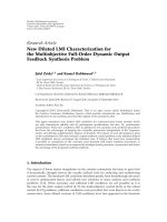
Figure 1: Simple morphological profile with 2 openings and 2
closings. In the profile shown, circular structuring elements are used
with radius increment 4 (r
= 4, 8 pixels). The image processed is
part of Figure 4(a).
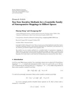
Profile from PC1 Profile from PC2
Combined profile
Figure 2: Extended morphological profile of two images. Each

of the original profiles has 2 openings and 2 closings. A circular
structuring element with radius increment 4 was used (r
= 4,8).
The image processed is part of Figure 4(a).
where γ
(i)
R
is the opening by reconstruction with a structuring
element (SE) of size i,andp is the total number of openings.
Also, the CP at pixel x of image f is defined as a p-
dimensional vector:
CP
i
(x) = φ
(i)
R
(x), ∀i ∈ [0, p], (2)
where φ
(i)
R
is the closing by reconstruction with an SE of size
i.Clearly,wehaveCP
0
(x) = OP
0
(x) = f (x). By collating the
OP and the CP, the MP of image f is defined as a 2p +1-
dimensional vector:
MP(x)
=


CP
p
(x), , f (x), ,OP
p
(x)

. (3)
An example of MP is shown in Figure 1. Thus, from a
single image a multivalued image results. The dimension of
this image corresponds to the number of transformations.
For application to hyperspectral data, characteristic images
need to be extracted. In [26], it was suggested to use several
principal components (PCs) of the hyperspectral data for
such a purpose. Hence, the MP is applied on the first
PCs, corresponding to a certain amount of the cumulative
variance, and a stacked vector is built using the MP on each
PC. This yields the extended morphological profile (EMP).
Following the previous notation, the EMP is a q(2p +1)-
dimensional vector:
EMP(x)
=

MP
PC
1
(x), ,MP
PC
q
(x)


,(4)
where q is the number of retaining PCs. An example of an
EMP is shown in Figure 2.
As stated in the introduction, PCA does not fully handle
the spectral information. Previous works using alternative
feature reduction algorithms, such as independent compo-
nent analysis (ICA), have led to equivalent results in terms
of classification accuracy [31]. In this article, we propose
the use of the KPCA rather than PCA for the construction
of the EMP, that is, the first kernel PCs (KPCs) are used to
build the EMP. The assumption is that much more spectral
information will be captured by the KPCA than with the
PCA. The next section presents the KPCA and how the KPCA
is applied to hyperspectral remote sensing images.
3. Kernel Principal Component Analysis
3.1. Kernel PCA Problem. In this section, a brief description
is given of kernel principal component analysis for feature
reduction on remote sensing data. The theoretical founda-
tion may be found in [20, 32, 33].
The starting point is a set of pixel vectors x
i
∈ R
n
, i ∈
[1, , ]. Conventional PCA solves the eigenvalue problem:
λv
= Σ
x
v,subjecttov

2
= 1, (5)
where Σ
x
= E[x
c
x
T
c
] ≈ (1/( − 1))


i=1
(x
i
− m
x
)(x
i
−m
x
)
T
,
and x
c
is the centered vector x. A projection onto the first m
principal components is performed as x
pc
= [v

1
|···|v
m
]
T
x.
To capture higher-order statistics, the data can be
mapped onto another space H (from now on,
R
n
is called
the input space and H the feature space):
Φ :
R
n
−→ H
x
−→ Φ(x),
(6)
where Φ is a function that may be nonlinear, and the only
restriction on H is that it must have the structure of a
reproducing kernel Hilbert space (RKHS), not necessarily of
finite dimension. PCA in H can be performed as in the input
space, but thanks to the kernel trick [34], it can be performed
directly in the input space. The kernel PCA (KPCA) solves
the following eigenvalue problem:
λα
= Kα,subjecttoα
2
=

1
λ
,(7)
where K is the kernel matrix constructed as follows:
K
=
⎛
⎜
⎜
⎜
⎜
⎜
⎜
⎜
⎝
k

x
1
, x
1

···
k

x
1
, x



k

x
2
, x
1

···
k

x
2
, x


.
.
.
.
.
.
.
.
.
k

x

, x
1


··· k

x

, x


⎞
⎟
⎟
⎟
⎟
⎟
⎟
⎟
⎠
. (8)
The function k is the core of the KPCA. It is a positive
semidefinite function on
R
n
that introduces nonlinearity
into the processing. This is usually called a kernel. Classic
kernels are the polynomial kernel, q
∈ R
+
and p ∈ N
+
,

k(x, y)
=

x, y
R
+ q

p
,(9)
and the Gaussian kernel, σ
∈ R
+
,
k(x, y)
= exp

−
x −y
2
2σ
2

. (10)
4 EURASIP Journal on Advances in Signal Processing
−0.2
0
0.2
0.4
0.6
0.8

−0.20 0.20.40.60.8
(a)
−0.8
−0.6
−0.4
−0.2
0
0.2
0.4
0.6
−0.8 −0.6 −0.4 −0.20 0.20.40.60.8
(b)
−0.5
0
0.5
−0.8 −0.6 −0.4 −0.20 0.20.40.60.8
(c)
−0.2
0
0.2
0.4
0.6
0.8
−0.20 0.20.40.60.8
(d)
−0.2
0
0.2
0.4
0.6

0.8
−0.20 0.20.40.60.8
(e)
−0.2
0
0.2
0.4
0.6
0.8
−0.20 0.20.40.60.8
(f)
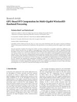
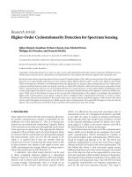
Figure 3: PCA versus KPCA. (a) Three Gaussian clusters, and their projection onto the first two kernel principal components with (b)
a Gaussian kernel and (c) a polynomial kernel. (d), (e), and (f) represent, respectively, the contour plot of the projection onto the first
component for the PCA, the KPCA with Gaussian kernel, and the KPCA with a polynomial kernel. Note how with the Gaussian kernel the
first component “picks out” the individual clusters [20]. The intensity of the contour plot is proportional to the value of the projection, that
is, light gray indicates that Φ
1
kpc
(x) has a high value.
As with conventional PCA, once (7) has been solved,
projection is then performed:
Φ
m
kpc
(x) =


i=1
α
m

i
k

x
i
, x

. (11)
Note it is assumed that K is centered, otherwise it can be
centered as [35]
K
c
= K −1

K − K1

+ 1

K1

(12)
where 1

is a square matrix such as (1

)
ij
= 1/.
3.2. PCA versus KPCA. Let us start by recalling that the
PCA relies on a simple generative model. The n observed

variables result from a linear transformation of m Gaussianly
distributed latent variables, and thus it is possible to recover
the latent variable from the observed one by solving (5).
To better understand the link and the difference between
PCA and KPCA, one must note that the eigenvectors of
Σ
x
can be obtained from those of XX
T
,whereX =
[x
1
, x
2
, , x

]
T
[36]. Consider the eigenvalue problem:
γu
= XX
T
u,subjecttou
2
= 1. (13)
The left part is multiplied by X
T
giving
γX
T

u = X
T
XX
T
u,
γX
T
u = ( −1)Σ
x
X
T
u,
γ

X
T
u = Σ
x
X
T
u,
(14)
which is the eigenvalue problem (5): v
= X
T
u.Butv
2
=
u
T

XX
T
u = γu
T
u = γ
/
=1. Therefore, the eigenvectors of Σ
x
can be computed from eigenvectors of XX
T
as v = γ
−0.5
X
T
u.
The matrix XX
T
is equal to
⎛
⎜
⎜
⎜
⎜
⎜
⎜
⎜
⎝

x
1

, x
1

···

x
1
, x



x
2
, x
1

···

x
2
, x


.
.
.
.
.
.
.

.
.

x

, x
1

···

x

, x


⎞
⎟
⎟
⎟
⎟
⎟
⎟
⎟
⎠
, (15)
which is the kernel matrix with a linear kernel: k(x
i
, x
j
) =


x
i
, x
j

R
n
. Using the kernel trick k(x
i
, x
j
) =Φ(x
i
), Φ(x
j
)
H
,
K can be rewritten in a similar form as (15)
⎛
⎜
⎜
⎜
⎜
⎜
⎜
⎜
⎝


Φ

x
1

, Φ

x
1

H
···

Φ

x
1

, Φ

x


H

Φ

x
2


, Φ

x
1

H
···

Φ

x
2

, Φ

x


H
.
.
.
.
.
.
.
.
.

Φ


x


, Φ

x
1

H
···

Φ

x


, Φ

x


H
⎞
⎟
⎟
⎟
⎟
⎟
⎟

⎟
⎠
. (16)
From (15)and(16), the advantage of using KPCA comes
from an appropriate projection Φ of
R
n
onto H . In this
space, the data should better match the PCA model. It is clear
that the KPCA shares the same properties as the PCA, but in
different space.
To illustrate how the KPCA works, a short example is
given here. Figure 3(a) represents three Gaussian clusters.
The conventional PCA would result in a rotation of the
space, that is, the three clusters would not be identified.
Figures 3(b) and 3(c) represent the projection onto the first
two kernel principal components (KPCs). Using a Gaussian
kernel, the structure of the data is better captured than with
PCA: a cluster can be clearly identified on the first KPC
EURASIP Journal on Advances in Signal Processing 5
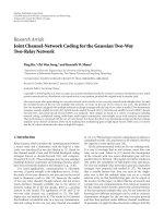
(a) (b)
(c)
Figure 4: ROSIS data. (a) University Area, (b) Pavia Center. HYDICE data: (c) Washington DC.
(see Figure 3(e)). However, the obtained results are different
with a polynomial kernel. In that case, the clusters are not as
well identified as with the Gaussian kernel. Finally, from the
contour plots, Figures 3(e) and 3(f), the nonlinear projection
of the KPCA can be seen while linear projection with the PCA
can be seen in Figure 3(d). The contour plots are straight
lines with PCA while curved lines with KPCA.

This synthetic experiment reveals the importance of
the choice of kernels. In the next section, the selection of
a kernel adapted to hyperspectral remote sensing data is
discussed.
3.3. KPCA Applied to Remote Sensing Data. To compute the
KPCA, it is first necessary to choose the kernel function
to build the kernel matrix. This is a difficult task which is
still under consideration in the “kernel method” community
[37]. However, when considering the two classical kernels
in (9)and(10), one can choose between them using some
prior information. If it is known that higher-order statistics
are relevant to discriminate samples, a polynomial kernel
should be used. But under the Gaussian cluster assumption,
the Gaussian kernel should be used. Hyperspectral remote
sensing data are known to be well approximated by a
Gaussian distribution [7], and thus in this work a Gaussian
kernel is used.
With the Gaussian kernel, one hyperparameter needs
to be tuned, that is, σ.Theσ controls the width of
the exponential function. A too small value of σ causes
k(x
i
, x
j
) = 0, i
/
= j, that is, each sample is considered as an
individual cluster. While a too high value causes k(x
i
, x

j
) = 1,
that is, all samples are considered neighbors. Thus, only one
cluster can be identified. Several strategies can be used, from
cross-validation to density estimation [38].Thechoiceof
σ should reflect the range of the variables, to be able to
detect samples that belong to the same cluster from those
that belong to others clusters. A simple, yet effective, strategy
was employed in this experiment. It consists of stretching
the variables between 0 and 1, and fixing σ to a value that
provides good results according to some criterion. For a
remote sensing application, the number of extracted KPCs
should be of same order than the number of species/classes
in the image. From our experiments, σ was fixed at 4 for all
data sets.
Section 5 presents experimental results using the KPCA
on real hyperspectral images. As stated in the introduction,
the aim of using the KPCA is to extract relevant features
for the construction of the EMP. The classification of such
features with the support vector machines is described in the
next section.
4. Support Vector Machines
The support vector machines (SVMs) are surely one of
the most used kernel learning algorithms. They perform
robust nonlinear classification of samples using the kernel
trick. The idea is to find a separating hyperplane in some
feature space induced by the kernel function while all the
computations are done in the original space [39]. A good
introduction to SVM for pattern recognition may be found
6 EURASIP Journal on Advances in Signal Processing

in [40]. Given a training set S
={(x
1
, y
1
), ,(x

, y

)}∈
R
n
×{−1; 1}, the decision function is found by solving the
convex optimization problem:
max
a
g(a) =


i=1
α
i
−
1
2


i,j=1
α
i

α
j
y
i
y
j
k

x
i
, x
j

subject to 0 ≤ α
i
≤ C and


i=1
α
i
y
i
= 0,
(17)
where α are the Lagrange coefficients, C a constant that
is used to penalize the training errors, and k the kernel
function. Same than KPCA, classic effective kernels are (9)
and (10). A short comparison of kernels for remotely sensed
image classification may be found in [41]. Advanced kernel

functions can be constructed using some prior [42].
When the optimal solution of (17) is found, that is, α
i
,
the classification of a sample x is achieved by observing to
which side of the hyperplane it belongs:
y
= sgn



i=1
α
i
y
i
k

x
i
, x

+ b

. (18)
SVMs are designed to solve binary problems where the
class labels can only take two values:
±1. For a remote-
sensing application, several species/classes are usually of
interest. Various approaches have been proposed to address

this problem. They usually combine a set of binary classifiers.
Two main approaches were originally proposed for C-class
problems [35].
(i) One-versus-the-Rest. C binary classifiers are applied on
each class against all the others. Each sample is assigned to
the class with the maximum output.
(ii) Pairwise Classification. C(C
− 1)/2 binary classifiers are
applied on each pair of classes. Each sample is assigned to
the class getting the highest number of votes. A vote for a
given class is defined as a classifier assigning the pattern to
that class.
Pairwise classification has proved more suitable for large
problems [43]. Even though the number of classifiers used is
larger than for the one-ver sus-the-rest approach, the whole
classification problem is decomposed into much simpler
ones. Therefore, the pairwise approach was used in our
experiments. More advanced approaches applied to remote
sensing data can be found in [44].
SVMs are primarily a nonparametric method, yet some
hyperparameters do need to be tuned before optimization.
In the Gaussian kernel case, there are two hyperparameters:
C the penalty term and σ the width of the exponential. This is
usually done by a cross-validation step, where several values
are tested. In our experiments, C is fixed to 200 and σ
2
∈
{
0.5, 1, 2, 4} is selected using 5-fold cross validation. The
SVM optimization problem was solved using the LIBSVM

[45]. The range of each feature was stretched between 0 and
1.
5. Experiments
Three real data sets were used in the experiments. They are
detailed in the following. The original hyperspectral data are
termed “Raw” in the rest of the paper.
5.1. Data Set. Airborne data from the reflective optics system
imaging spectrometer (ROSIS-03) optical sensor are used for
the first two experiments. The flight over the city of Pavia,
Italy was operated by the Deutschen Zentrum f
¨
ur Luft- und
Raumfahrt (DLR, the German Aerospace Agency) within
the context of the HySens project, managed and sponsored
by the European Union. According to specifications, the
ROSIS-03 sensor provides 115 bands with a spectral coverage
ranging from 0.43 to 0.86 μm. The spatial resolution is 1.3 m
per pixel. The two data sets are:
(1) university Area: the first test set is around the
Engineering School at the University of Pavia. It
is 610
× 340 pixels. Twelve channels have been
removed due to noise. The remaining 103 spectral
channels are processed. Nine classes of interest are
considered: tree, asphalt, bitumen, gravel, metal
sheet, shadow, bricks, meadow, and soil;
(2) Pavia center: the second test set is the center of Pavia.
The Pavia center image was originally 1096
× 1096
pixels. A 381 pixel wide black band in the left-

hand part of image was removed, resulting in a “two
part” image of 1096
× 715 pixels. Thirteen channels
have been removed due to noise. The remaining
102 spectral channels are processed. Nine classes of
interest are considered: water, tree, meadow, brick,
soil, asphalt, bitumen, tile, and shadow.
Airborne data from the hyperspectral digital imagery col-
lection experiment (HYDICE) sensor was used for the
third experiments. The HYDICE was used to collect data
from flightline over the Washington DC Mall. Hyper-
spectral HYDICE data originally contained 210 bands in
the 0.4–2.4 μm region. Channels from near-infrared and
infrared wavelengths are known to contained more noise
than channel from visible wavelengths. Noisy channels due
to water absorption have been removed, and the set consists
of 191 spectral channels. The data were collected in August
1995, and each channel has 1280 lines with 307 pixels each.
Seven information classes were defined, namely, roof, road,
grass, tree, trail, water, and shadow. Figure 4 shows false color
images for all the data sets.
Available training and test sets for each data set are given
in Tables 1, 2,and3. These are selected pixels from the data
by an expert, corresponding to a predefined species/classes.
Pixels from the training set are excluded from the test set in
each case and vice versa.
The classification accuracy was assessed with
(i) an overall accuracy (OA) which is the number of
well-classified samples divided by the number of test
samples,

(ii) an average accuracy (AA) which represents the
average of class classification accuracy,
EURASIP Journal on Advances in Signal Processing 7
Table 1: Information classes and training/test samples for the
University Area data set.
Class Samples
No Name Train Test
1 Asphalt 548 6641
2 Meadow 540 18649
3 Gravel 392 2099
4 Tree 524 3064
5 Metal Sheet 265 1345
6 Bare Soil 532 5029
7 Bitumen 375 1330
8 Brick 514 3682
9 Shadow 231 947
Total 3921 42776
Table 2: Information classes and training/test samples for the Pavia
Center data set.
Class Samples
No Name Train Test
1 Water 824 65971
2 Tree 820 7598
3 Meadow 824 3090
4 Brick 808 2685
5 Bare soil 820 6584
6 Asphalt 816 9248
7 Bitumen 808 7287
8 Tile 1260 42826
9 Shadow 476 2863

Total 7456 148152
Table 3: Information classes and training/test samples for the
Washington DC Mall data set.
Class Samples
No. Name Train Test
1 Roof 40 3794
2 Road 40 376
3 Trail 40 135
4 Grass 40 1888
5 Tree 40 365
6 Water 40 1184
7 Shadow 40 57
Total 280 6929
(iii) a kappa coefficient of agreement (κ) which is the
percentage of agreement corrected by the amount of
agreement that could be expected due to chance alone
[7],
(iv) a class accuracy which is the percentage of correctly
classified samples for a given class.
These criteria were used to compare classification results
and were computed using a confusion matrix. Furthermore,
the statistical significance of differences was computed using
McNemar’s test, which is based upon the standardized
normal test statistic [46]:
Z
=
f
12
− f
21


f
12
+ f
21
, (19)
where f
12
indicates the number of samples classified correctly
by classifier 1 and incorrectly by classifier 2. The difference in
accuracy between classifiers 1 and 2 is said to be statistically
significant if
|Z| > 1.96. The sign of Z indicates whether
classifier 1 is more accurate than classifier 2 (Z>0) or vice
versa (Z<0). This test assumes that the training and the test
samples are related and is thus adapted to the analysis since
the training and test sets were the same for each experiment
for a given data set.
5.2. Spectral Feature Extraction. Solving the eigenvalues
problem (5) for each data set yields the results reported
in Tabl e 4. Looking at the cumulative eigenvalues, in each
ROSIS case, three principal components (PCs) reach 95% of
total variance. After the PCA transformation, the dimension-
ality of the new representation of the University Area data
set and the Pavia Center is 3, if the threshold is set to 95%
of the cumulative variance. The results for the third data
set are somewhat different. Acquired from a higher range
of wavelengths, more noise is contained in the data and
more bands were removed by comparison to the ROSIS data.
That explains why more PCs are needed, that is, 40 PCs, to

reach 95% of the cumulative variance. But from the table,
it can be clearly seen that the first two PCs contain most
of the information. This means that by using second-order
information, the hyperspectral data can be reduced to a two-
or three-dimensional space. But, as experiments will show,
hyperspectral richness is not fully handled using only the
mean and variance/covariance of the data.
Ta bl e 5 shows the variance and the cumulative variance
for the three data sets when KPCA is applied. The kernel
matrix in each case was constructed using 5000 randomly
selected samples. From the table, it can be seen that more
kernel principal components (KPCs) are needed to achieve
the same amount of variance as for the conventional PCA.
For the University data set, the first 12 KPCs are needed
to achieve 95% of the cumulative variance, 11 for the
Washington DC data set and only 10 for the Pavia Center
data set. That may be an indication that more information
is extracted and the KPCA is more robust to the noise,
since a reasonable number of features are extracted from the
Washington DC data set.
To test this assumption, the mutual information (MI)
between each (K)PC has been computed. The classical
correlation coefficient was not used since the PCA is optimal
for that criterion. For comparison, the normalized MI was
computed: I
n
(x, y) = I(x, y)/(

I(x, x)


I(y, y)). The MI
is used to test independence between two variables, and
intuitively the MI measures the information that the two
variables share. An MI close to 0 indicates independence,
while a high MI indicates dependence and consequently
similar information. Figure 5 presents the MI matrices,
which represents the MI for each pair of extracted features
8 EURASIP Journal on Advances in Signal Processing
Table 4: PCA: Eigenvalues and cumulative variance in percentages for the three hyperspectral data sets.
Pavia center University area Washington DC
Component % Cum. % % Cum. % % Cum. %
1 72.85 72.85 64.85 64.85 53.38 53.38
2 21.03 93.88 28.41 93.26 18.65 72.03
3 04.23 98.11 05.14 98.40 03.83 75.87
4 00.89 99.00 00.51 98.91 02.00 77.87
5 00.30 99.30 00.25 99.20 00.66 78.00
Table 5: KPCA: Eigenvalues and cumulative variance in percent for the two hyperspectral data sets (KPCA).
Pavia center University area Washington DC
Component % Cum. % % Cum. % % Cum. %
1 43.94 43.94 31.72 31.72 40.99 40.99
2 21.00 64.94 26.04 57.76 20.18 61.17
3 15.47 80.41 19.36 75.12 13.77 74.95
4 05.23 85.64 06.76 81.88 05.99 80.94
5 03.88 89.52 04.31 86.19 05.22 86.16
with both PCA and KPCA, for the Washington DC data set.
From Figure 5(a), PCs number 4 to 40 contain more or less
the same information since they correspond to a high MI.
Although uncorrelated, these features are still dependent.
This phenomenon is due to the noise contained in the data
which is not Gaussian [6] and is distributed over several PCs.

From Figure 5(a), KPCA is less sensitive to the noise, that is,
in the feature space the data match better the PCA model and
the noise tends to be Gaussian. Note that with KPCA, only
the first 11 KPCs are retained against 40 with conventional
PCA.
To visually assess what is contained in each different
(K)PC, Figure 6 represents the first, second, and thirtieth PC
for both the PCA and the KPCA. It can be seen that
(1) the extracted PCs are different (all the images have
been linearly stretched between 0 and 255 for the
purpose of visualization),
(2) the thirtieth PC contains only noise, while the
thirtieth KPC still contains some information and
spatial structure can be detected with the EMP.
In conclusion of this section, the KPCA can extract
more information from the hyperspectral data than the
conventional PCA, and is robust to the noise that can
affect remote sensing data. The next question is: Is this
information useful for the purpose of classification? In
the next section, experiments are conducted using features
extracted by the PCA and the KPCA, for the classification or
for the construction of the EMP.
5.3. Classification of Remote Sensing Data. Several experi-
ments were conducted to evaluate KPCs as a suitable feature
for (1) the classification of remote sensing images and (2)
the construction of the EMP. For the first item, linear
SVM are used to perform the classification. The aim is to
investigate whether the data are easily classified after the PCA
40
35

30
25
20
15
10
5
510152025303540
0.2
0.4
0.6
0.8
1
(a) PCA
40
35
30
25
20
15
10
5
5 10152025303540
0.2
0.4
0.6
0.8
1
(b) KPCA
Figure 5: Mutual Information matrices for the Washington DC data
set.

or the KPCA. Therefore a linear classifier is used to limit
its influence on the results. For the EMP, as state in the
introduction, too much information are lost during the PCA,
and experiments should confirm that the KPCA extracts
more information. In the following, an analysis of the results
foreachdatasetsisprovided.
EURASIP Journal on Advances in Signal Processing 9
(a) 1st PC (b) 2nd PC (c) 30th PC (d) 1st KPC (e) 2nd KPC (f) 30th KPC
Figure 6: (Kernel) Principal component for the Washington DC data set.
In each case, the EMP was constructed using (K)PCs
corresponding to 95% of the cumulative variance. A circular
SE with a step size increment of 2 was used. Four openings
and closings were computed for each (k)PC, resulting in an
EMP of dimension 9
× m (m being the number of retained
(K)PCs).
5.3.1. University Area. The results are reported in Ta ble 6 and
the Z tests in Tab le 7 . Regarding the global accuracies, the
linear classification of PCA and KPCA features is significantly
better than what is obtained by directly classifying the
spectral data. Although feature extraction helps for the
classification whatever the algorithm, the difference between
PCA- and KPCA-based results is not statistically significant,
that is,
|Z|≤1.96.
The nonlinear SVM yield to a significant improvement
in terms of accuracy when compared to linear SVM. The
KPCA features are the more accurately classified, with an OA
equal to 79.81%. The raw data are classified using the non-
linear SVM and a significant improvement of the accuracy

is achieved. However, the PCA features lose a lot of spectral
information as compared to the KPCA and the classification
of the PCA feature is less accurate that the one obtained using
the all spectral channel or KPCs.
EMP constructed with either PCs or KPCs outperformed
all others approaches in classification. The κ is increased by
15% with EMP
PCA
and by 20% with EMP
KPCA
. The statistical
difference of accuracy Z
=−35.33 clearly demonstrates the
benefit of using the KPCA rather than the PCA.
Regarding the class accuracy, the highest improvements
were obtained for class 1 (Asphalt), class 2 (Meadow)and
class 3 (Gravel). For these classes, the original spectral infor-
mation was not sufficient and the morphological processing
provided additional useful information.
Thematic maps obtained with the non-linear SVM
applied to the Raw data, EMP
PCA
and EMP
KPCA
are reported
in Figure 7. For instance, it can be seen that building in
the top right corner (made of bitumen) is detected with
EMP
KPCA
while totally missed with EMP

PCA
.Theregion
corresponding to class 2, meadow, are more homogeneous
in the image Figure 7(c) than in the two others images.
5.3.2. Pavia Center. TheresultsarereportedinTa bl e 8
and the Z tests in Ta b le 9 . The Pavia Center data set was
easier to classify since even the linear SVM provide very
high classification accuracy. Regarding the global accuracies,
feature extraction does not improve the accuracies, for
both linear and non-linear SVM. Yet, the KPCA performs
significantly better than the PCA in terms of accuracies;
even more, the KPCA + linear SVM outperform the PCA +
nonlinear SVM. Even high accuracy for linear SVM, the use
of nonlinear SVM is still justified since significantly higher
accuracies are obtained with Z
= 2.07.
Again, the very best results are obtained with EMP
for both the PCA and the KPCA. However, the statistical
significance of difference is lower than with the University
Area data set although it is still significant: Z
=−2.90.
For the class accuracy, most of the improvement is done
on class 4 (Br ick ) which is almost perfectly classified with the
EMP
KPCA
and the nonlinear SVM.
5.3.3. Washington DC. TheresultsarereportedinTa bl e 10
and the Z tests in Tabl e 11 . The ground truth of the
Washington DC data sets is limited, resulting in a very small
training and test sets. As mentioned in Section 5.2, the data

contain non-Gaussian noise, and the number of PCs needed
to reach 95% of the cumulative variance is high.
From the global accuracies, all the different approaches
perform similarly. It is confirmed with the Z test. Linear and
nonlinear SVM applied on the raw data sets provide the same
results, and it is the same for the KPCA features. Despite
high number of feature, PCA and linear SVM provide
poor results. But surprisingly, one of the best results are
obtained with PCA features and nonlinear SVM. It means
that nonlinear can properly deal with the noise contained in
the PCs.
10 EURASIP Journal on Advances in Signal Processing
Table 6: Classification results for the University Area data set.
SVM & linear kernel SVM & Gaussian kernel
Feature Raw PCA KPCA Raw PCA KPCA EMP
PCA
EMP
KPCA
Nb of features 103 3 12 103 3 12 27 108
OA 76.40 78.32 78.22 79.48 78.38 79.81 92.04 96.55
AA 85.04 81.77 87.58 88.14 85.16 87.60 93.21 96.23
κ 68.67 71.95 72.96 74.47 72.73 74.79 89.65 95.43
1 81.44 72.63 85.44 84.35 78.83 82.63 94.60 96.23
2 59.61 80.61 63.89 66.20 71.31 68.81 88.79 97.58
3 75.94 59.31 71.18 71.99 67.84 67.98 73.13 83.66
4 81.09 97.55 96.83 98.01 98.17 98.14 99.22 99.35
5 99.55 99.55 99.48 99.48 99.55 99.41 99.55 99.48
6 93.94 58.82 90.61 93.12 78.62 92.34 95.23 92.88
7 89.62 84.74 90.90 91.20 88.12 90.23 98.87 99.10
8 84.79 82.84 91.99 92.26 86.28 91.88 99.10 99.46

9 99.47 99.89 97.89 96.62 97.68 97.47 90.07 98.31
Table 7: Statistical Significance of Differences in Classification (Z) for the University Area data set. Each case of the table represents Z
rc
where r is the row and c is the column.
Z
rc
SVM & linear kernel SVM & Gaussian kernel
Raw PCA KPCA Raw PCA KPCA EMP
PCA
EMP
KPCA
Linear
Raw
−13.68 −18.91 −23.76 −13.88 −23.28 −73.77 −89.61
PCA 13.68 0.41
−4.81 −0.27 −6.41 −57.49 −83.49
KPCA 18.91
−0.41 −8.14 −0.69 −10.15 −64.42 −82.07
Gaussian
Raw 23.76 4.81 8.14 5.14
−2.49 −60.28 −78.69
PCA 13.88 0.27 0.69
−5.14 −7.19 −59.90 −82.43
KPCA 23.28 6.41 10.15 2.49 7.19
−59.45 −78.34
EMP
PCA
73.77 57.49 64.42 60.28 59.90 59.45 −35.33
EMP
KPCA

89.61 83.49 82.07 78.69 82.43 78.34 35.33
(a) (b) (c)
Figure 7: Thematic map obtained with the University Area. (a) Raw data, (b) EMP
PCA
,(c)EMP
KPCA
. The classification was done by SVM
with a Gaussian kernel. The color-map is as follows: asphalt, meadow, gravel, tree, metal sheet, bare soil, bitumen, brick, and shadow.
EURASIP Journal on Advances in Signal Processing 11
Table 8: Classification results for the Pavia Center data set.
SVM & linear kernel SVM & Gaussian kernel
Feature Raw PCA KPCA Raw PCA KPCA EMP
PCA
EMP
KPCA
Nb of features 102 3 10 102 3 10 27 90
OA 97.60 96.54 97.39 97.67 96.99 97.32 98.81 98.87
AA 95.42 92.34 94.38 95.60 93.56 94.40 98.14 98.25
κ 96.62 95.14 96.32 96.71 95.76 96.23 98.32 98.41
1 98.41 98.82 98.57 98.35 98.80 98.49 99.07 98.91
2 93.43 85.56 90.94 91.23 87.33 89.06 92.67 92.01
3 96.57 94.82 95.15 96.76 94.98 95.40 96.38 96.31
4 88.27 81.15 83.87 88.45 82.94 82.50 99.70 99.59
5 94.41 88.97 94.99 93.97 95.23 94.55 99.39 99.77
6 95.17 94.82 95.36 96.32 94.72 96.06 98.48 99.24
7 93.18 88.14 91.12 96.01 89.24 94.50 97.98 98.58
8 99.38 98.30 99.43 99.40 98.83 99.07 99.68 99.89
9 99.93 99.93 99.97 99.93 99.93 99.93 99.93 99.55
Table 9: Statistical significance of differences in classification (Z) for the Pavia center data set. Each case of the table represents Z
rc

where r
is the row and c is the column.
Z
rc
SVM & linear kernel SVM & Gaussian kernel
Raw PCA KPCA Raw PCA KPCA EMP
PCA
EMP
KPCA
Linear
Raw 26.74 6.13
−2.07 15.15 7.87 −32.71 −34.26
PCA
−26.74 −21.01 −27.71 −13.00 −19.70 −52.92 −54.27
KPCA
−6.13 21.01 −9.45 12.19 2.38 −37.30 −40.23
Gaussian
Raw 2.07 27.71 9.45 18.9 13.30
−32.25 −35.36
PCA
−15.15 13.00 −12.19 −18.91 −10.13 −45.78 −47.67
KPCA
−7.78 19.70 −2.38 −13.30 10.13 −39.03 −42.41
EMP
PCA
32.71 52.92 37.30 32.25 45.78 39.03 −2.90
EMP
KPCA
35.26 54.27 40.23 35.36 47.67 42.41 2.90
As with the previous experiments, best accuracies are

achieved with the EMP, but also with the PCA, and nonlinear
SVM. The difference in the three classification is not
statistically significant, as can be seen from Ta bl e 11.
Regarding the class accuracies, the class 7, shadow,is
perfectly classifier only by EMP
KPCA
.
5.3.4. Discussion. As stated in the introduction, the first
objective of this paper was to assess the relevance of the
KPCA as a feature reduction tool for hyperspectral remote
sensing imagery. From the experiments with the linear SVM,
the classification accuracies are at least similar (one case) or
better (two cases) with the features extracted with KPCA thus
legitimizing KPCA as a suitable alternative to PCA. The same
conclusion can be drawn when the classification is done with
nonlinear SVM.
The second objective was to use the KPCs for the con-
struction of an EMP. Comparison with an EMP constructed
with PCs is significantly favorable to KPCA for two cases.
For the most difficult data, the University Area, the OA
reaches 96.55% with EMP
KPCA
whichis4.5%morethanwith
EMP
PCA
. This results strengthen the use of KPCA against
PCA.
For the third data set, which contains non-Gaussian
noise, the KPCA clearly deals better with the noise than PCA.
Furthermore, a reasonable number of KPCs were extracted,

that is, 10 compared to 40 extracted with PCA.
In this paper, the Gaussian kernel was used for both the
KPCA and the nonlinear SVM. For the KPCA, the statistical
behavior of the data has justified this choice and for the
SVM previous experiments have shown that the Gaussian
kernel produce the best accuracies. However, when no or
little prior information is available from the data, the choice
of the kernel for the KPCA is not straightforward. A Gaussian
kernel is in general a good initial choice. However, the best
results are surely obtained with a more appropriate kernel.
The computational load for the KCPA is increased by
comparison to the PCA. Both involve matrix inversions
which are o(d
3
), where d is the number of variable for
the PCA and the number of samples for the KPCA; clearly
d
PCA
 d
KPCA
, for example, for the Washington DC data
set d
PCA
= 191 and d
KPCA
= 5000. Thus, even if the KPCA
12 EURASIP Journal on Advances in Signal Processing
Table 10: Classification results for the Washington DC data set.
SVM & linear kernel SVM & Gaussian kernel
Feature Raw PCA KPCA Raw PCA KPCA EMP

PCA
EMP
KPCA
Nb of features 103 40 11 103 40 11 360 99
OA 98.16 97.85 98.18 98.16 98.84 98.18 98.64 98.73
AA 98.89 95.95 97.20 96.89 97.65 97.20 98.02 99.39
κ 97.35 96.90 97.38 97.35 98.32 97.38 98.04 98.16
1 97.05 96.50 97.08 97.05 98.10 97.08 97.52 97.52
2 98.08 99.28 98.32 98.08 98.28 98.32 99.52 98.80
3 100 99.43 100 100 99.43 100 100 100
4 100 100 100 100 100 100 100 100
5 98.02 98.77 98.02 98.02 99.26 98.02 99.51 99.51
6 99.51 97.88 99.35 99.59 99.84 99.35 99.92 99.92
7 85.57 79.38 87.65 85.57 87.63 87.63 89.69 100
Table 11: Statistical Significance of Differences in Classification (Z) for the Washington DC data set. Each case of the table represents Z
rc
where r is the row and c is the column.
Z
rc
SVM & linear kernel SVM & Gaussian kernel
Raw PCA KPCA Raw PCA KPCA EMP
PCA
EMP
KPCA
Linear
Raw 2.81
−0.57 0 −6.03 −0.57 −5.68 −6.78
PCA
−2.81 −3.00 −2.81 −7.84 −3.00 −8.00 −7.98
KPCA 0.57 3.00 0.57

−5.81 0 −5.39 −6.63
Gaussian
Raw 0 2.81
−0.57 −6.03 −0.57 −5.68 −6.78
PCA 6.03 7.84 5.81 6.03 5.81 2.06 1.02
KPCA 0.57 3.00 0 0.57 5.81
−5.39 −6.63
EMP
PCA
5.68 8.00 5.39 5.68 −2.06 5.39 −1.40
EMP
KPCA
6.78 7.98 6.63 6.78 −1.02 6.63 1.40
involves a well-known matrix algorithm, the computational
load (both in terms of CPU and memory) is higher than with
the PCA.
6. Conclusions
This paper presents KPCA-based methods with application
to the analysis of hyperspectral remote sensing data. Two
important issues have been considered: (unsupervised fea-
ture extraction by means of the KPCA, (construction of
the EMP with KPCs. Comparisons were done with the
conventional PCA. Comparisons in terms of classification
accuracies with a linear SVM demonstrate that KPCA
extracts more informative features and is more robust to
the noise contained in the hyperspectral data. Classification
results of the EMP built with the KPCA significantly
outperforms those obtained with the EMP with the PCA.
Practical conclusions are that, where possible, the KPCA
should be used in preference to the PCA because the KPCA

extracts more useful features for the purpose of classification.
However, one limitation of the KPCA is its computational
complexity, related to the size of the kernel matrix, which can
limit the number of samples used. In our experiments, 5000
random samples were used leading to satisfactory results.
Our current investigations are oriented to nonlinear
independent component analysis, such as kernel ICA [47],
for the construction of the EMP and to a sparse KPCA in
order to reduce the complexity [48].
Acknowledgments
The authors thank the reviewers for their many helpful
comments. This research was supported in part by the
Research Fund of the University of Iceland and the Jules
Verne Program of the French and Icelandic Governments
(PAI EGIDE).
References
[1] M. Fauvel, J. Chanussot, and J. A. Benediktsson, “Decision
fusion for hyperspectral classification,” in Hyperspectral Data
Exploitation: Theory and Applications, C I. Chang, Ed., John
Wiley & Sons, New York, NY, USA, 2007.
[2] C. Chang, Hyperspect ral Imaging: Techniques for Spectral
Detection and Classification, Kluwer Academic Publishers,
Dordrecht, The Netherlands, 2003.
[3] C. Lee and D. A. Landgrebe, “Analyzing high-dimensional
multispectral data,” IEEE Transactions on Geoscience and
Remote Sensing, vol. 31, no. 4, pp. 792–800, 1993.
EURASIP Journal on Advances in Signal Processing 13
[4] L. Jimenez and D. A. Landgrebe, “Supervised classification in
high dimensional space: geometrical, statistical and asymp-
totical properties of multivariate data,” IEEE Transactions on

Systems, Man, and Cybernetics, Part B,vol.28,no.1,pp.39–
54, 1993.
[5] G. Hughes, “On the mean accuracy of statistical pattern
recognizers,” IEEE Transactions on Information Theory, vol. 14,
no. 1, pp. 55–63, 1968.
[6] D. A. Landgrebe, Signal Theory Methods in Multispectral
Remote Sensing, John Wiley & Sons, Hoboken, NJ, USA, 2003.
[7] J. A. Richards and X. Jia, Remote Sensing Digital Image Analysis:
An Introduction, Springer, New York, NY, USA, 1999.
[8] N. Keshava, “Distance metrics and band selection in hyper-
spectral processing with applications to material identification
andspectrallibraries,”IEEE Transactions on Geoscience and
Remote Sensing, vol. 42, no. 7, pp. 1552–1565, 2004.
[9] C.
¨
Unsalan and K. L. Boyer, “Linearized vegetation indices
basedonaformalstatisticalframework,”IEEE Transactions on
Geoscience and Remote Sensing, vol. 42, no. 7, pp. 1575–1585,
2004.
[10] K S. Park, S. Hong, P. Park, and W D. Cho, “Spectral con-
tent characterization for efficient image detection algorithm
design,” EURASIP Journal on Advances in Signal Processing,
vol. 2007, Article ID 82874, 14 pages, 2007.
[11] A. Jain and D. Zongker, “Feature selection: evaluation, appli-
cation, and small sample performance,” IEEE Transactions on
Pattern Analysis and Machine Intelligence, vol. 19, no. 2, pp.
153–158, 1997.
[12] P. Somol, P. Pudil, J. Novovi
ˇ
cov

´
a, and P. Pacl
´
ık, “Adaptive float-
ing search methods in feature selection,” Pattern Recognition
Letters, vol. 20, no. 11–13, pp. 1157–1163, 1999.
[13] S. B. Serpico and L. Bruzzone, “A new search algorithm for
feature selection in hyperspectral remote sensing images,”
IEEE Transactions on Geoscience and Remote Sensing, vol. 39,
no. 7, pp. 1360–1367, 2001.
[14] B. Guo, S. R. Gunn, R. I. Damper, and J. D. B. Nelson, “Band
selection for hyperspectral image classification using mutual
information,” IEEE Geoscience and Remote Sensing Letters, vol.
3, no. 4, pp. 522–526, 2006.
[15] H. Kwon and N. M. Nasrabadi, “A comparative analysis of
kernel subspace target detectors for hyperspectral imagery,”
EURASIP Journal on Advances in Signal Processing, vol. 2007,
Article ID 29250, 13 pages, 2007.
[16] M. Lennon, M
´
ethodes d’analyse d’images hyperspectrales,
exploitation du capteur a
´
eroport
´
e CASI pour des applications
de cartographies agro-environnementale en Bretagne,Ph.D.
dissertation, Universit
´
e de Rennes, Rennes, France, 2002.

[17] L. Journaux, X. Tizon, I. Foucherot, and P. Gouton, “Dimen-
sionality reduction techniques: an operational comparison on
multispectral satellite images using unsupervised clustering,”
in Proceedings of the 7th Nordic Signal Processing Symposium
(NORSIG ’06), pp. 242–245, Reykjavik, Iceland, June 2006.
[18] M. Lennon, G. Mercier, M. C. Mouchot, and L. Hubert-Moy,
“Curvilinear component analysis for nonlinear dimensionality
reduction of hyperspectral images,” in Image and Signal
Processing for Remote Sensing VII, vol. 4541 of
Proceedings of
SPIE, pp. 157–168, Toulouse, France, September 2002.
[19] A. Hyv
¨
arinen, J. Karhunen, and E. Oja, Independent Compo-
nent Analysis, John Wiley & Sons, New York, NY, USA, 2001.
[20] B. Sch
¨
olkopf, A. Smola, and K R. M
¨
uller, “Nonlinear com-
ponent analysis as a Kernel eigenvalue problem,” Neural
Computation, vol. 10, no. 5, pp. 1299–1319, 1998.
[21] M. Fauvel, J. Chanussot, and J. A. Benediktsson, “Kernel
principal component analysis for feature reduction in hyper-
spectrale images analysis,” in Proceedings of the 7th Nordic
Signal Processing Symposium (NORSIG ’06), pp. 238–241,
Reykjavik, Iceland, June 2006.
[22] M. Pesaresi and J. A. Benediktsson, “A new approach for
the morphological segmentation of high-resolution satellite
imagery,” IEEE Transactions on Geoscience and Remote Sensing,

vol. 39, no. 2, pp. 309–320, 2001.
[23] J. A. Benediktsson, M. Pesaresi, and K. Arnason, “Classifica-
tion and feature extraction for remote sensing images from
urban areas based on morphological transformations,” IEEE
Transactions on Geoscience and Remote Sensing,vol.41,no.9,
part 1, pp. 1940–1949, 2003.
[24] P. Soille, Morphological Image Analysis: Principles and Applica-
tions, Springer, New York, NY, USA, 2nd edition, 2003.
[25] A. Plaza, P. Mart
´
ınez, J. Plaza, and R. P
´
erez, “Dimensionality
reduction and classification of hyperspectral image data using
sequences of extended morphological transformations,” IEEE
Transactions on Geoscience and Remote Sensing,vol.43,no.3,
pp. 466–479, 2005.
[26] J. A. Benediktsson, J. A. Palmason, and J. R. Sveinsson,
“Classification of hyperspectral data from urban areas based
on extended morphological profiles,” IEEE Transactions on
Geoscience and Remote Sensing, vol. 43, no. 3, pp. 480–491,
2005.
[27] J. A. Palmason, J. A. Benediktsson, J. R. Sveinsson, and J.
Chanussot, “Fusion of morphological and spectral informa-
tion for classification of hyperspectal urban remote sensing
data,” in Proceedings of IEEE Internat ional Conference on
Geoscience and Remote Sensing Symposium (IGARSS ’06),pp.
2506–2509, Denver, Colo, USA, July-August 2006.
[28] M. Fauvel, J. Chanussot, J. A. Benediktsson, and J. R.
Sveinsson, “Spectral and spatial classification of hyperspectral

data using SVMs and morphological profiles,” in Proceedings
of IEEE International Conference on Geoscience and Remote
Sensing Symposium (IGARSS ’07), pp. 1–12, Barcelona, Spain,
October 2008.
[29] T. G
´
eraud and J B. Mouret, “Fast road network extraction in
satellite images using mathematical morphology and Markov
random fields,” EURASIP Journal on Applied Signal Processing,
vol. 2004, no. 16, pp. 2503–2514, 2004.
[30] X. Jin and C. H. Davis, “Automated building extraction
from high-resolution satellite imagery in urban areas using
structural, contextual, and spectral information,” EURASIP
Journal on Applied Signal Processing, vol. 2005, no. 14, pp.
2196–2206, 2005.
[31] J. A. Palmason, Classification of hyperspectral data from urban
areas, M.S. thesis, Faculty of Engineering, University of
Iceland, Reykjavik, Iceland, 2005.
[32] B. Sch
¨
olkopf, S. Mika, C. J. C. Burges, et al., “Input space ver-
sus feature space in kernel-based methods,” IEEE Transactions
on Neural Networks, vol. 10, no. 5, pp. 1000–1017, 1999.
[33] K R. M
¨
uller, S. Mika, G. R
¨
atsch, K. Tsuda, and B. Sch
¨
olkopf,

“An introduction to kernel-based learning algorithms,” IEEE
Transactions on Neural Networks, vol. 12, no. 2, pp. 181–201,
2001.
[34] N. Aronszajn, “Theory of reprodusing kernel,” Tech. Rep.
11, Division of Engineering Sciences, Harvard University,
Cambridge, Mass, USA, 1950.
[35] B. Sch
¨
olkopf and A. J. Smola, Learning with Kernels: Support
Vector Machines, Regularization, Optimization, and Beyond,
MIT Press, Cambridge, Mass, USA, 2002.
14 EURASIP Journal on Advances in Signal Processing
[36] J. A. Lee and M. Verleysen, Nonlinear Dimensionality Reduc-
tion, Springer, New York, NY, USA, 2007.
[37] J. Shawe-Taylor and N. Cristianini, Kernel Methods for Pattern
Analysis, Cambridge University Press, Cambridge, UK, 2004.
[38] M. Fauvel, Spectral and spatial methods for the classification of
urban remote sensing data, Ph.D. dissertation, Institut National
Polytechnique de Grenoble, Reykjavik, Iceland, 2007.
[39] V. Vapnik, Statistical Learning Theory, John Wiley & Sons, New
York, NY, USA, 1998.
[40] C. J. C. Burges, “A tutorial on support vector machines for
pattern recognition,” Data Mining and Knowledge Discovery,
vol. 2, no. 2, pp. 121–167, 1998.
[41] M. Fauvel, J. Chanussot, and J. A. Benediktsson, “Evaluation
of kernels for multiclass classification of hyperspectral remote
sensing data,” in Proceedings of IEEE International Conference
on Acoustics, Speech, and Signal Processing (ICASSP ’06), vol. 2,
pp. 813–816, Toulouse, France, May 2006.
[42] Q. Yong and Y. Jie, “Modified kernel functions by geodesic

distance,” EURASIP Journal on Applied Signal Processing, vol.
2004, no. 16, pp. 2515–2521, 2004.
[43] C W. Hsu and C J. Lin, “A comparison of methods for
multiclass support vector machines,” IEEE Transactions on
Neural Networks, vol. 13, no. 2, pp. 415–425, 2002.
[44] F. Melgani and L. Bruzzone, “Classification of hyperspectral
remote sensing images with support vector machines,” IEEE
Transactions on Geoscience and Remote Sensing,vol.42,no.8,
pp. 1778–1790, 2004.
[45] C C. Chang and C J. Lin, “LIBSVM: a library for support
vector machines,” 2001, />∼cjlin/
libsvm.
[46] G. M. Foody, “Thematic map comparison: evaluating the
statistical significance of differences in classification accuracy,”
Photogrammetric Engineering & Remote Sensing,vol.70,no.5,
pp. 627–633, 2004.
[47] F. R. Bach and M. I. Jordan, “Kernel independent component
analysis,” The Journal of Machine Learning Research, vol. 3, pp.
1–48, 2002.
[48] L. K. Saul and J. B. Allen, “Periodic component analysis:
an eigenvalue method for representing periodic structure in
speech,” in Advances in Neural Information Processing Systems
13, T. K. Leen, T. G. Dietterich, and V. Tresp, Eds., pp. 807–813,
MIT Press, Cambridge, Mass, USA, 2001.