Báo cáo hóa học: " Research Article Simulation of Two-Dimensional Supersonic Flows on Emulated-Digital CNN-UM" docx

Hindawi Publishing Corporation
EURASIP Journal on Advances in Signal Processing
Volume 2009, Article ID 923404, 11 pages
doi:10.1155/2009/923404
Research Article
Simulation of Two-Dimensional Supersonic Flows on
Emulated-Digital CNN-UM
S
´
andor Kocs
´
ardi,
1
Zolt
´
an Nagy,
2
´
Arp
´
ad Cs
´
ık,
3
and P
´
eter Szolgay
2, 4
1
Department of Image Processing and Neurocomputing, Faculty of Information Technology,
University of Pannonia, Egyetem 10, 8200 Veszpr

´
em, Hungary
2
Cellular Sensory and Wave Computing Laboratory, Computer and Automation Research Institute,
Hungarian Academy of Sciences, 1518 Budapest, Hungary
3
Department of Mathematics and Computational Sciences, Sz
´
echenyi Istv
´
an University, 9026 Gy
˝
or, Hungary
4
Faculty of Information Technology, P
´
azm
´
any P
´
eter Catholic University, 1083 Budapest, Hungary
Correspondence should be addressed to S
´
andor Kocs
´
ardi,
Received 25 September 2008; Accepted 7 January 2009
Recommended by Victor M. Brea
Computational fluid dynamics (CFD) is the scientific modeling of the temporal evolution of gas and fluid flows by exploiting
the enormous processing power of computer technology. Simulation of fluid flow over complex-shaped objects currently requires

several weeks of computing time on high-performance supercomputers. A CNN-UM-based solver of 2D inviscid, adiabatic, and
compressible fluids will be presented. The governing partial differential equations (PDEs) are solved by using first- and second-
order numerical methods. Unfortunately, the necessity of the coupled multilayered computational structure with nonlinear, space-
variant templates does not make it possible to utilize the huge computing power of the analog CNN-UM chips. To improve the
performance of our solution, emulated digital CNN-UM implemented on FPGA has been used. Properties of the implemented
specialized architecture is examined in terms of area, speed, and accuracy.
Copyright © 2009 S
´
andor Kocs
´
ardi et al. This is an open access article distributed under the Creative Commons Attribution
License, which permits unrestricted use, distribution, and reproduction in any medium, provided the original work is properly
cited.
1. Introduction
The CNN paradigm is a natural framework to describe
the behavior of locally interconnected dynamical systems
which have an array structure [1]. Therefore, it possesses
an inherent potential in the fields of computational fluid
dynamics and numerical analysis [2]. Unfortunately, analog
CNN-UM chips suffer from technical limitations dimin-
ishing their efficiency in such practical applications. Their
most notable deficiencies are the low precision (8 bits)
and restricted usability in applications requiring nonlinear,
space-variant templates in a multilayered structure. How-
ever, by implementing the concepts behind the CNN-UM
technology on reconfigurable architectures, the cell model
can be modified according to the numerical simulation of the
physical phenomena under consideration [3, 4]. Simulation
of a 2D compressible flow on CNN-UM was reported in
[5] but this solution used customized floating-point number

representation inside the arithmetic unit. Unfortunately, area
requirements of the floating-point arithmetic units are quite
high, therefore, parallelism of the arithmetic unit needs
to be reduced which has a negative impact on computing
performance.
In this paper, we focus on the numerical solution of the
same hyperbolic system of the nonlinear Euler equations but
using fixed-point numbers. Our aim is to find some optimal
computational architecture satisfying the functional require-
ments with minimal required precision, while driving com-
puting power toward its maximum level. Thus, we intend to
perform the operations with the highest possible parallelism.
The structure of the paper is the following. In Section 2,
we recall the theoretical bases of compressible, adiabatic fluid
flows. The details of the numerical discretization technique
are described in Section 3. The optimized Falcon processor
with the CNN templates and the optimized fixed-point
arithmetic unit are given in Sections 4 and 5.InSection 6, the
2 EURASIP Journal on Advances in Signal Processing
accuracy analysis of the fixed- and floating-point solutions
is presented and the features of their implementation on
FPGA units are investigated. Finally, conclusions are drawn
in Section 7.
2. Fluid Flows
A wide range of industrial processes and scientific phenom-
ena involve gas or fluids flows over complex obstacles, for
example, air flow around vehicles and buildings and the
flow of water in the oceans or liquid in BioMEMS. In engi-
neering applications, the temporal evolution of nonideal,
compressible fluids is quite often modeled by the system of

Navier-Stokes equations. It is based on the fundamental laws
of mass, momentum, and energy conservation, extended
by the dissipative effects of viscosity, diffusion, and heat
conduction. By neglecting all these nonideal processes and
assuming adiabatic variations, we obtain the Euler equations
[6, 7], describing the dynamics of dissipation-free, inviscid,
compressible fluids. They are a coupled set of nonlinear
hyperbolic partial differential equations, in conservative
form expressed as
∂ρ
∂t
+
∇·(ρv) = 0,
∂(ρv)
∂t
+
∇·

ρvv +

Ip

=
0,
∂E
∂t
+
∇·

(E + p)v


= 0,
(1)
where t denotes time,
∇is the nabla operator, ρ is the density,
u, v are the x-andy-component of the velocity vector v,
respectively, p is the pressure of the fluid,

I is the identity
matrix, and E is the total energy density defined as
E
=
p
γ −1
+
1
2
ρv
·v. (2)
In (2), the value of the ratio of specific heats is taken to
be γ
= 1.4. For later use, we introduce the conservative
state vector U
= [ρ, ρu, ρv, E]
T
, the set of primitive variables
P
= [ρ, u, v, E]
T
, and the speed of sound c =


γp/ρ.Itis
also convenient to merge (1) into hyperbolic conservation
law form in terms of U and the flux tensor,
F
=
⎛
⎜
⎜
⎝
ρv
ρvv + Ip
(E + p)v
⎞
⎟
⎟
⎠
,(3)
as
∂U
∂t
+
∇·F = 0. (4)
3. Discretization of the Governing Equations
Since logically structured arrangement of data is fundamen-
tal for the efficient operation of the FPGA-based implemen-
tations, we consider explicit finite volume discretization of
the governing equations over structured grids employing a
simple numerical flux function. Indeed, the corresponding
rectangular arrangement of information and the choice of

multilevel temporal integration strategy ensure the contin-
uous flow of data through the CNN-UM architecture. In
the followings, we recall the basic properties of the mesh
geometry, and the details of the considered first- and second-
order schemes.
3.1. The Geometry of the Mesh. For the sake of simplicity,
in this paper, we only consider rectangular computational
domains labeled by Ω. The sides of the rectangle are a and
b units long. We divide Ω into M
× N nonoverlapping
rectangular finite volumes (cells) of equal sizes. The volume
situated in the ith column and the jth row is indexed by
(i, j). The resolution of the mesh in the x- and the y-
directions coinciding with the length of the cells’ edges are
Δx
= a/M and Δy = b/N, thus the volume of the cell (i, j)
is V
i,j
. Following the finite volume methodology, we store all
components of the volume-averaged state vector U
i,j
at the
mass center of cell (i, j).
3.2. The Discretization Scheme. Application of the finite
volume discretization method leads to the following semidis-
crete form of governing equations (4)
dU
i,j
dt
=−

1
V
i,j

f
F
f
·n
f
,(5)
where the summation is meant for all four faces of cell
(i, j), F
f
is the flux tensor evaluated at face f and n
f
is
the outward pointing normal vector of face f scaled by the
length of the face. Let us consider face f in a coordinate
frame attached to the face, such that its x-axis is normal
to f (see Figure 1). Face f separates cell L (left) and cell R
(right). In this case, the F
f
·n
f
scalar product equals to the
x-component of F(F
x
) multiplied by the area of the face. In
order to stabilize the solution procedure, artificial dissipation
has to be introduced into the scheme. According to the

standard procedure, this is achieved by replacing the physical
flux tensor by the numerical flux function F
N
containing
the dissipative stabilization term. A finite volume scheme is
characterized by the evaluation of F
N
which is the function
of both U
L
and U
R
. In this paper, we employ the simple and
robust Lax-Friedrichs numerical flux function defined as
F
N
=
F
L
+ F
R
2
−

|u|+ c

U
R
−U
L

2
. (6)
In the last equation, F
L
= F
x
(U
L
)andF
R
= F
x
(U
R
)and
notations
|u| and |c| represent the average value of the u
velocity component and the speed of sound at an interface,
respectively. The temporal derivative is discretized by the
first-order forward Euler method
dU
i,j
dt
=
U
n+1
i,j
−U
n
i,j

Δt
,(7)
where U
n
i,j
is the known value of the state vector at time level
n, U
n+1
i,j
is the unknown value of the state vector at time level
n +1,andΔt is the time step.
EURASIP Journal on Advances in Signal Processing 3
Cell LL Cell L Cell R Cell RR
n
f
Interface f
Figure 1: Interface with the normal vector and the cells required in
the computation.
By working out the algebra described so far, it leads to
the discrete form of the governing equations to compute the
numerical flux term F and the dissipation term D,
F
ρ,n
i
=
ρu
n
C
+ ρu
n

i
2
, i
= E, W,
F
ρu,n
i
=

ρu
2
+ p

n
C
+

ρu
2
+ p

n
i
2
, i
= E, W,
F
ρu,n
i
=

ρuv
n
C
+ ρuv
n
i
2
, i
= N,S,
F
ρv,n
i
=
ρuv
n
C
+ ρuv
n
i
2
, i
= E, W,
F
ρv,n
i
=

ρv
2
+ p


n
C
+

ρv
2
+ p

n
i
2
, i
= N,S,
F
E,n
i
=
(E + p)u
n
C
+(E + p)u
n
i
2
, i
= E, W,
F
E,n
i

=
(E + p)v
n
C
+(E + p)v
n
i
2
, i
= N,S,
D
ρ,n
i
=

|u|+ c

ρ
n
i
−ρ
n
C
2
, i
= E, N,
D
ρ,n
i
=


|u|+ c

ρ
n
C
−ρ
n
i
2
, i
= W,S,
D
ρu,n
i
=

|u|+ c

ρu
n
i
−ρu
n
C
2
, i
= E, N,
D
ρu,n

i
=

|u|+ c

ρu
n
C
−ρu
n
i
2
, i
= W,S,
D
ρv,n
i
=

|u|+ c

ρv
n
i
−ρv
n
C
2
, i
= E, N,

D
ρv,n
i
=

|u|+ c

ρv
n
C
−ρv
n
i
2
, i
= W,S,
D
E,n
i
=

|u|+ c

E
n
i
−E
n
C
2

, i
= E, N,
D
E,n
i
=

|u|+ c

E
n
C
−E
n
i
2
, i
= W,S.
(8)
Complex terms in the equation were marked with only one
super- and subscript for better understanding, for example,
(ρu
2
+ p)
n
C
is equal to ρ
n
C
(u

n
C
)
2
+ p
n
C
. Additionally, in the
subscripts E, W, N,andS denote the eastern, western,
northern, and southern interfaces of the examined cell.
Finally, in (9), the update scheme for each layer can be
seen based on (8),
ρ
n+1
C
= ρ
n
C
−
Δt
Δx

F
ρ,n
E
−F
ρ,n
W
+ D
ρ,n

E
−D
ρ,n
W

−
Δt
Δy

F
ρ,n
N
−F
ρ,n
S
+ D
ρ,n
N
−D
ρ,n
S

,
ρu
n+1
C
= ρu
n
C
−

Δt
Δx

F
ρu,n
E
−F
ρu,n
W
+ D
ρu,n
E
−D
ρu,n
W

−
Δt
Δy

F
ρu,n
N
−F
ρu,n
S
+ D
ρu,n
N
−D

ρu,n
S

,
ρv
n+1
C
= ρv
n
C
−
Δt
Δx

F
ρv,n
E
−F
ρv,n
W
+ D
ρv,n
E
−D
ρv,n
W

−
Δt
Δy


F
ρv,n
N
−F
ρv,n
S
+ D
ρv,n
N
−D
ρv,n
S

,
E
n+1
C
= E
n
C
−
Δt
Δx

F
E,n
E
−F
E,n

W
+ D
E,n
E
−D
E,n
W

−
Δt
Δy

F
E,n
N
−F
E,n
S
+ D
E,n
N
−D
E,n
S

.
(9)
The overall accuracy of the scheme can be raised to
second order if the spatial and the temporal derivatives are
calculated by a second-order approximation. One way to

satisfy the latter requirement is to perform a piecewise linear
extrapolation of the primitive variables P
L
and P
R
at the
two sides of the interface in (6). This procedure requires the
introduction of additional cells with respect to the interface,
that is, cell LL (left to cell L) and cell RR (right to cell R)
as shown in Figure 1. With these labels, the reconstructed
primitive variables are
P
L
= P
L
+
g
L

δP
L
, δP
C

2
,
P
R
= P
R

−
g
R

δP
C
, δP
R

2
,
(10)
with
δP
L
= P
L
−P
LL
,
δP
C
= P
R
−P
L
,
δP
R
= P

RR
−P
R
.
(11)
while g
L
and g
R
are the limiter functions. The scheme
without limitation yields acceptable second-order time-
accurate approximation of the solution, only if the variations
in the flow field are smooth. However, the integral form of
the governing equations admits discontinuous solutions as
well, and in an important class of applications the solution
contains shocks. In order to capture these discontinuities
without spurious oscillations, in (10) we apply the minmod
limiter function, also
g
L

δP
L
, δP
C

=
⎧
⎪
⎪

⎪
⎨
⎪
⎪
⎪
⎩
δP
L
,if


δP
L


<


δP
C


, δP
L
δP
C
> 0,
δP
C
,if



δP
C


<


δP
L


, δP
L
δP
C
> 0,
0, if δP
L
δP
C
≤ 0.
(12)
The function g
R
(δP
C
, δP
R

) can be defined analogously.
4 EURASIP Journal on Advances in Signal Processing
The temporal derivative is discretized by the standard
two-stage Runge-Kutta method [8]. During the second-order
update procedure, the primitive variables (ρ, u, v,andp)are
computed from the conservative variables (ρ, ρu, ρv,andE)
and extrapolated by using the limiter function. The resulting
variables are used to compute the spatial derivatives (9)and
time is advanced by half time step according to the second-
order Runge-Kutta method. Finally, the whole procedure is
repeated to compute the next timestep.
A vast amount of experience has shown that these
equations provide a stable discretization of the governing
equations if the time step obeys the following Courant-
Friedrichs-Lewy (CFL) condition:
Δt
≤ min
(i,j)∈([1,M]×[1,N])
min

Δx, Δy



u
i,j


+ c
i,j

. (13)
4.ImplementationonFalconCNN-UM
Architecture
The Falcon architecture [9] is an emulated digital implemen-
tation of CNN-UM array processor which uses the full signal
range model. On this architecture, the flexibility of simu-
lators and computational power of analog architectures are
mixed. Not only the size of templates and the computational
precision can be configured, but space-variant and nonlinear
templates can also be used.
The Euler equations were solved by a modified Falcon
processor array in which the arithmetic unit has been
changed according to the discretized governing equations.
Since each CNN cell has only one real output value, four
layers are required to represent the variables ρ, ρu, ρv,and
E. In case of a simple first-order forward Euler temporal
discretization, the nonlinear CNN templates acting on the
ρu layer can easily be taken from the discretized equations.
Equations (14) show templates in which cells of different
layers at positions (k, l) are connected to the cell of layer ρu
at position (i, j),
A
ρu
1
=
1
2Δx
⎡
⎢
⎢

⎣
00 0
ρu
2
+ p 0 −(ρu
2
+ p)
00 0
⎤
⎥
⎥
⎦
,
A
ρu
2
=
1
2Δx
⎡
⎢
⎢
⎣
0 −ρuv 0
000
0 ρuv 0
⎤
⎥
⎥
⎦

,
A
ρu
3
=
1
2Δx
⎡
⎢
⎢
⎣
0 ρv 0
ρu
−2ρu − 2ρv ρu
0 ρv 0
⎤
⎥
⎥
⎦
.
(14)
Thetemplatevaluesforρ, ρv,andE layers can be defined
analogously.
In accordance with (9), we have designed four complex
circuits. These are able to update the values of the conserva-
tive state vector of a cell in every clock cycle using emulated
digital CNN-UM architecture. The arithmetic unit for the
computation of the ρu layer is shown in Figure 2.Theρuu+p,
ρuv, ρu,andρv terms can be reused during the computation
of the neighboring cells and they should be computed only

once in each iteration step. This solution requires additional
memory elements but greatly reduces the area requirement
of the arithmetic unit.
Other trick can be applied if we choose the ratio of
Δt and Δx or Δy to be integer power of two because the
multiplication with Δt/Δx and Δt/Δy can be done by shifts so
we can eliminate several multipliers from the hardware and
additionally the area requirements will be greatly reduced.
Unfortunately, in the second-order case, limiter function
should be used on the primitive variables and the con-
servative variables are computed from these results. The
limitedvalueswillbedifferent for the four interfaces and
cannot be reused in the computation of the neighboring cells.
Therefore, this approach does not make it possible to derive
CNN templates for the solution. However, a specialized
arithmetic unit still can be designed to compute the second-
order update scheme described in the previous section
directly.
In accordance with the discretized governing equations,
we have designed a complex circuit which is able to update
the values of the conservative state vector of a cell in every
clock cycle using emulated digital CNN-UM architecture.
The main building blocks of the proposed unit are shown in
Figure 3(a). From the blocks, two identical arithmetic cores
can be built according to the two steps of the second-order
Runge-Kutta method. In order to get the conservative state
values at time level n + 1, the two identical units need to
be applied successively. The arithmetic core computing ρu
value after the first step can be seen in Figure 3(b).Two
similar units (F

N
and F
E
) are required to compute the flux
value at the North and South or East and West interfaces
while four instances of the third unit (D
E
)isrequiredto
compute the artificial diffusion term. Inputs of these units
are connected to the output of the appropriate limiter units.
In order to achieve the highest possible clock speed during
the computation, pipelining technique and parallel working
hardware units have been used.
5. Fixed-Point Arithmetic Unit
FPGA implementation of the previously described arith-
metic unit using floating-point IP cores was reported in [5].
The results show that even computing with 32-bit single
precision numbers, the currently available largest FPGAs are
required for the implementation. Size of the arithmetic unit
is greatly increased by the area requirements of the floating-
point adders.
Some previous studies proved the effectiveness of fixed-
point numbers during the solution of simple PDEs [10]. In
case of simple PDEs, all bits computed during the evaluation
of the derivative are kept and rounding is carried out at the
last step when the state value is updated. Unfortunately, this
method cannot be used in our case because the bit width of
the partial results is growing quickly as shown in Figure 4(a).
To reduce the bit width inside the arithmetic unit and reduce
EURASIP Journal on Advances in Signal Processing 5

ρu u p ρu v
∗∗
ρu ρu c ρu ρu c ρu ρu c ρu ρu c
∗∗∗∗
−−−−
+
+
+
+
+
+
++
Shift reg.
Shift reg.
Shift reg.
Shift reg.
Figure 2: The proposed arithmetic unit to compute the derivative or ρu layer in the solution using first-order Lax-Friedrichs approximation
method.
ρ
n
C
u
n
C
u
n
C
p
n
C

ρ
n
E
u
n
E
u
n
E
p
n
E
∗∗
∗∗
ρu
n
C
ρu
n
E
F
E
ρu
n
C
ρu
n
N
F
N

D
E
−
++
+
+
Flux at interface E (F
E
) Flux at interface N (F
N
)
∗∗
∗
∗
∗
ρ
n
C
u
n
C
v
n
C
ρ
n
N
u
n
N

v
n
N
ρu
n
E
ρu
n
C
u
n
EC
Dissipative term at
interface E (D
E
)
(a)
F
E
F
W
F
N
F
S
D
E
D
W
D

N
D
S
ρu
n+1/2
C
−−−−
−
−
++
ρu
n
C
(b)
Figure 3: (a) The main building blocks of the proposed arithmetic unit, (b) the whole arithmetic unit built from the main blocks.
6 EURASIP Journal on Advances in Signal Processing
4.28 3.29 3.29
7.57
5.27
10.86
4.28 3.29 3.29
7.57
5.27
10.86
10.86 10.86
11.86
F
E
+
++

∗∗
∗∗
ρ
n
C
u
n
C
u
n
C
p
n
C
ρ
n
E
u
n
E
u
n
E
p
n
E
(a)
4.28 3.29 3.29
7.31
5.27

9.6
4.28 3.29 3.29
7.31
5.27
9.6
9.27 9.27
10.26
F
E
+
++
∗∗
∗∗
ρ
n
C
u
n
C
u
n
C
p
n
C
ρ
n
E
u
n

E
u
n
E
p
n
E
(b)
Figure 4: Bit width of the fixed-point arithmetic unit to compute
F
E
, (a) without optimization, (b) optimized by using interval
arithmetic (bit width is denoted by (integer width) . (fractional
width)).
area requirements, rounding is required. However, it should
be carried out very carefully because important information
required to accurately compute the derivative of a state value
may be lost during improper rounding.
One possible solution to determine the number of frac-
tional bits required during the computation is to use interval
arithmetic [11] and compute the error of the operation along
with the result. The basic arithmetic operations computed
in interval arithmetic have the following form (m:computer
representation of the number, ε: computer representation of
the error):
m
1
±ε
1
+ m

2
±ε
2
=

m
1
+ m
2

±

ε
1
+ ε
2

,
(15a)
m
1
±ε
1
−m
2
±ε
2
=

m

1
−m
2

±

ε
1
+ ε
2

,
(15b)
m
1
±ε
1
×m
2
±ε
2
=

m
1
×m
2

±


ε
1


m
2


+


m
1


ε
2
+ ε
1
ε
2

,
(15c)
m
1
±ε
1
÷m
2

±ε
2
=

m
1
m
2

±

ε
1
+


m
1
/m
2


ε
2


m
2



−
ε
2

. (15d)
The error of the addition and subtraction is simply
the sum of the error of the operands while in the case
of multiplication and division, the error of the results also
depends on the value of the operands.
In our case, we assume that a priori information is
available about the maximum value of the input variables
(this is usually true in engineering applications), which can
be used to determine the number of integer and fractional
bits. We also assume that the least significant bit (LSB) of the
input values is erroneous, therefore, ε is set to 2
−LSB
.Error
of the additions and subtractions can be easily determined
by using (15a)-(15b). However, to determine the error of
the multiplication and division, the value of the operands
are also required which is not known in advance. Therefore,
a worst case analysis of the accuracy of the arithmetic unit
should be carried out by computing the minimum and
maximum values and the minimum and maximum errors of
each partial result. The number of integer bits is computed
from the maximal value while the number of fractional bits
can be computed form the minimum error value by using the
following equations:
int
=


log
2
(2·max)

,
frac
=

−
log
2

ε
min

,
(15)
where int is the number of integer bits, frac is the number
of fractional bits, and max is the computed maximal value
of the partial result, while its minimum error is denoted
by ε
min
. The computed minimum error values represent the
theoretically achievable accuracy of the computation. The
LSB of the variable (and the smallest representable number
2
−LSB
) should be set to be in the same range as the computed
minimal error. If the number of fractional bits is smaller,

valuable information is lost. On the other hand, using more
fractional bits does not really improve the results. A small
part of the arithmetic unit after the optimization (assuming
ρ
min
= 0.2) is shown in Figure 4(b).
Without optimization, the results of the multiplications
are stored on 64 and 96 bits and the output of the arithmetic
unit (F
E
) is 97-bit wide. If the results are used later during
multiplications, the bit width is further increased and quickly
hits an unpractical size. Using the previously described
method, the width of the partial results can be significantly
reduced. The width of the multiplications is decreased by
26 bits while the width of the final result is reduced to 36 bits
from 97 bits. Area requirements of the arithmetic units are
significantly decreased by using these optimizations while the
operating frequency is improved.
6. Results and Performance
6.1. Area Requirements. During the implementation of the
first- and second-order method, customized precision fixed-
point arithmetic cores from Xilinx [12] are used. Implemen-
tation and testing of the previously described arithmetic unit
can be very time-consuming but using rapid prototyping
techniques and high-level hardware description languages
such as Handel-C from agility [13]makeitpossibleto
EURASIP Journal on Advances in Signal Processing 7
0
2

4
6
8
10
12
14
16
×10
4
Number of slices
16 20 24 28 32 36 40 44 48 52 56 60 64
Bit width
1st order fix
2nd order fix
1st order fp
2nd order fp
(a)
0
200
400
600
800
1000
1200
1400
1600
1800
2000
Number of multipliers
16 20 24 28 32 36 40 44 48 52 56 60 64

Bit width
1st order fix
2nd order fix
1st order fp
2nd order fp
(b)
Figure 5: The area requirement of the fixed-point (fix) and
floating-point (fp) arithmetic units using different precisions.
develop the optimized arithmetic unit much faster than
using conventional VHDL-based approach.
Area requirement of the proposed fixed-point parallel
arithmetic units along with the area requirements of the
floating-point implementations [5] is shown in Figure 5
(in the following figures, bit width means the sum of the
integer and fractional bits of the fixed-point numbers and
the width of the mantissa bits in case of the floating-point
numbers). Due to the large area requirements of the floating-
point arithmetic units, especially the size of the floating-
point adders, only the low precision configurations of the
fully parallel first-order arithmetic unit can be realized even
on the currently available largest FPGAs (Virtex-5 SX240T
and LX330T). The fully parallel second-order arithmetic unit
cannot be implemented on these devices when floating-point
numbers are used. A possible solution could be for this
problem if the two steps of the Runge-Kutta method are
computed in two steps on the same arithmetic unit. In this
0
5
10
15

20
25
30
35
Number of arithmetic units
16 20 24 28 32 36 40 44 48 52 56 60 64
Bit width
1st order fix
2nd order fix
1st order fp
2nd order fp
∗
Figure 6: Number of implementable arithmetic units on Virtex-5
XC5VSX240T FPGA (
∗
half arithmetic unit—two clock cycles per
cell).
case, area requirements can be halved but the computing
performance is also halved.
Area requirements of the arithmetic unit can be signif-
icantly reduced, compared to the floating-point solution,
by using fixed-point numbers and using the optimization
method described in the previous section. The required
number of dedicated multipliers is about to be equal in
the case of fixed- and floating-point arithmetic. However,
using fixed-point arithmetic 2–5 times fewer logic elements
(slices) are required for the implementation of the first-
order arithmetic unit. In the second-order case, the area is
decreased more significantly by a factor of 5–15. The number
of implementable arithmetic units on the DSP optimized

Virtex-5 SX240T FPGA is summarized in Figure 6.
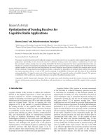
6.2. Test Setup. To show the efficiency of our solution, a
complex test case was used, in which a Mach 3 flow over a
forward facing step was computed. The simulated region is a
two-dimensional cut of a pipe which has closed at the upper
and lower boundaries, while the left and right boundaries
are open. The direction of the flow is from left to right
and the speed of the flow at the left boundary is 3-time the
speed of sound constantly. The solution contains shock waves
reflected from the closed boundaries. This problem was
solved by using the Handel-C simulation of the previously
described first- and second-order arithmetic units. In Figures
7 and 8, results of the computation using the derived
methods after 0.4 second, 1.2 seconds, and 4 seconds of
simulation time with 3.125 milliseconds (1/320 second) time
step are shown. In these figures, the dissipative property of
the first-order solution can be clearly recognized, while using
the second-order method the boundary of the shock waves
is sharp on the density distribution map. Because of the
applied rectangular, regular grid system a mask was necessary
to define the computational domain for the solution. The
grid points under the step are masked out and do not
take part in the solution resulting in dummy computing
cycles. This problem can be eliminated from the system
8 EURASIP Journal on Advances in Signal Processing
0
0.25
0.5
0.75
1

00.511.522.53
0.4 seconds
0.5
1
1.5
2
2.5
3
(a)
0
0.25
0.5
0.75
1
00.511.522.53
1.2 seconds
1
1.5
2
2.5
3
3.5
(b)
0
0.25
0.5
0.75
1
00.511.522.53
4 seconds

1
1.5
2
2.5
3
3.5
4
(c)
Figure 7: First-order solution of the Mach 3 flow on an 80 × 240
array after 0.4, 1.2, and 4 seconds of simulation time.
with the implementation of the multiblock technique when
the computational domain is divided into two parts at the
forward face of the step.
Reference solution for the previous problem computed
by the more accurate residual distribution upwind scheme
can be found in [14].
6.3. Performance. Performance of the architecture is deter-
mined by the maximum clock frequency and the num-
ber of arithmetic units. The huge amount of possible
configurations of the arithmetic unit does not enable to
carry out postlayout simulations in each case. Therefore,
performance data is provided by measuring the maximum
performance of the individual functional units. According
to the Xilinx data sheets, the floating-point arithmetic
cores can run on 350 MHz clock frequency in the case of
Virtex-5 FPGAs. Performance of the fixed-point arithmetic
0
0.25
0.5
0.75

1
00.511.522.53
0.4 seconds
0.5
1
1.5
2
2.5
3
3.5
(a)
0
0.25
0.5
0.75
1
00.511.522.53
1.2 seconds
1
2
3
4
5
(b)
0
0.25
0.5
0.75
1
00.511.522.53

4 seconds
1
1.5
2
2.5
3
3.5
4
(c)
Figure 8: Second-order solution of the Mach 3 flow on an 80 ×240
array after 0.4, 1.2, and 4 seconds of simulation time.
cores depends more on the width of the operands, and
about 400–550 MHz clock frequency can be achieved. Actual
clock frequency of a given configuration can be 0% to
20% smaller according to the utilization of the device
and due to changes in placement and routing. Expected
performance of the different arithmetic units compared to
an Intel Core2Duo microprocessor running on 2 GHz clock
frequency is summarized in Figure 9.
The computation of the Mach 3 problem lasts about
2419 seconds on the Core2Duo T7200 microprocessor using
first-order approximation while 10591 seconds are required
to compute the second-order result. This is equivalent to
approximately 1.3 million cell update per second for the first-
order method and 0.297 million cell update per second for
the second-order approach.
Using 32-bit fixed- and floating-point numbers, all
arithmetic units can be implemented on a Virtex-5 SX240T
FPGA. On this device, the first-order computation lasts
EURASIP Journal on Advances in Signal Processing 9

0.01
0.1
1
10
×10
4
Speedup
16 20 24 28 32 36 40 44 48 52 56 60 64
Bit width
1st order fix
2nd order fix
1st order fp
2nd order fp
∗
Figure 9: Speedup of the arithmetic unit implemented on Virtex-5
XC5VSX240T FPGA compared to a Core2Duo 2 GHz microproces-
sor (
∗
half arithmetic unit—two clock cycles per cell).
1E − 09
1E
−08
1E
−07
1E
−06
1E
−05
1E
−04

1E
−03
1E
−02
1E
−01
1E +00
1E +01
Infinity norm
16 20 24 28 32 36 40 44
Bit width
1st order fix
2nd order fix
1st order fp
2nd order fp
Figure 10: The infinity norm of the solutions.
approximately 0.78 second and 8.98 seconds in the fixed- and
floating-point cases , respectively, while in the second-order
case runtime is increased to 6.29 seconds and 17.97 seconds.
The first-order fixed-point arithmetic unit is 11-time faster
than its floating-point counterpart and more than 3000-time
faster than the Core2Duo microprocessor. In the second-
order case, the results are more balanced and the fixed-point
arithmetic unit is about 3-time faster than the floating-point
arithmetic but its performance is still superior compared to
the Core2Duo microprocessor.
Additionally, we tried to use performance data reported
in previous works, but fair comparison is hard because
different CFD models and discretization schemes are used.
Additionally different FPGA architectures are used during

the implementations. Smith and Schnore [15] published
an FPGA-based CFD solver, but they used 3D model and
0
0.25
0.5
0.75
1
00.511.522.53
0.4 seconds
−2.5
−2
−1.5
−1
−0.5
0
0.5
1
1.5
2
2.5
×10
−6
(a)
0
0.25
0.5
0.75
1
00.511.522.53
1.2 seconds

−8
−6
−4
−2
0
2
4
6
×10
−6
(b)
0
0.25
0.5
0.75
1
00.511.522.53
4 seconds
−1
−0.5
0
0.5
1
1.5
2
2.5
×10
−5
(c)
Figure 11: Error distribution of the first-order 32 bit fixed-point

solution of the Mach 3 problem after 0.4, 1.2, and 4 seconds of
simulation time.
smaller neighborhood during the computation. Additionally,
their architecture was implemented on several FPGAs. In the
solution of the Euler equations, they reported 24.6 GFlops
sustained performance on four Virtex-II 6000 FPGAs. Sano
et al. [16] used 2D systolic array to solve 2D flow problems
and reported 11.5 GFlops peak performance on an ALTERA
Stratix II FPGA. Sustained performance of our solution using
32-bit fixed-point numbers is 416 and 141 billion fixed-point
operations per second in the first- and second-order case,
respectively.
6.4. Accuracy of the Solutions. As described in Section 6.1,
area requirements of the arithmetic unit can be significantly
reduced by decreasing the precision of the state values.
10 EURASIP Journal on Advances in Signal Processing
0
0.25
0.5
0.75
1
00.511.522.53
0.4 seconds
−4
−3
−2
−1
0
1
2

3
4
5
×10
−6
(a)
0
0.25
0.5
0.75
1
00.511.522.53
1.2 seconds
−1.5
−1
−0.5
0
0.5
1
1.5
2
×10
−5
(b)
0
0.25
0.5
0.75
1
00.511.522.53

4 seconds
−2
0
2
4
6
8
10
12
×10
−5
(c)
Figure 12: Error distribution of the second-order 32 bit fixed-point
solution of the Mach 3 problem after 0.4, 1.2, and 4 seconds of
simulation time.
However, smaller precision results in less accurate solution.
Unfortunately, the exact solution of the Mach 3 problem
does not exist, therefore, the fixed- and customized-precision
floating-point results were compared to the 64-bit floating-
point result. The accuracy of the solutions was measured by
computing the infinity norm which is defined as
e
∞
= max
i


u
A
i

−u
E
i


, (16)
where u
A
i
is the exact (or in our case the 64-bit) solution,
while u
E
i
is the numerical approximation using the update
scheme with different fixed- and floating-point numbers.
The results of the comparison in the case of the Mach 3
problem are shown in Figure 10. Comparing the infinity
norm of the solutions to the largest density value (ρ
max
)in
the system, which was in this case about 10, a relative error
can be defined as
r
err
=

e
∞
ρ
max

. (17)
The error of the first-order fixed-point solution follows
the same trend as the error of the custom width floating-
point solution, but the error value in this case is about 4 times
higher. The larger error of the solution is balanced by the
smaller size and faster operation of the fixed-point arithmetic
unit, therefore, it is possible to slightly increase the bit width
and compute the results more accurately without loss of the
high computing performance.
In the second-order case, the error of the 32-bit fixed-
point solution is one-order higher compared to the error of
the 32-bit floating-point solution. Increasing the computing
precision to 40 bits just slightly increases the accuracy of
the solution, and the error compared to the 40-bit floating-
point solution is two orders higher. Further investigation is
required to find the roots of the different behaviors.
The results, which were calculated applying very low
precision (less than 24 bits), are unusable in engineering
applications, because the relative error is larger than 10
−2
in each case. Increasing the precision to 26–36 bits, the
relative error of our solution is in the range of 10
−4
–10
−6
.
These results are accurate enough to use in common
engineering applications. Accuracy of the solution can be
further increased by using higher precision to represent the
state values.

The distribution of the error of the 32-bit fixed-point
solutions in the first- and second-order case is presented in
Figures 11 and 12, respectively. As it can be seen in these
figures in the first-order case the distribution of the error
is quite smooth and has a maximum value near the shock
waves. In the second-order case, the maximum value of the
error is one-order larger and concentrated near the shock
waves.
7. Conclusion
The governing equations of the two-dimensional com-
pressible Newtonian flows were solved by using modified
emulated digital CNN architecture. The second-order Lax-
Friedrichs scheme was used during the solutions. The main
advantage of this method over the forward Euler method
which is used extensively in the computation of the CNN
dynamics is that this approximation is more robust in
the case of complex computational geometries and in the
presence of shock waves in the solutions.
The arithmetic unit was designed by using both fixed-
and floating-point number representations. Interval arith-
metic is used to optimally set the precision of the partial
results and to reduce the size of the fixed-point arithmetic
unit while preserving the accuracy of the solution. The
fixed- and floating-point solutions are compared in terms
of implementation area, accuracy of the solution, and
computing performance.
EURASIP Journal on Advances in Signal Processing 11
Implementation area of the arithmetic unit is signifi-
cantly decreased by the application of fixed-point numbers.
The proposed first-order fixed-point arithmetic unit can be

implemented on midsized gate arrays. Area requirements
of the second-order arithmetic unit are much higher and
the currently available largest FPGAs are required for the
implementation. The first-order solution using 32 bit fixed-
point numbers can be computed 3000 times faster compared
to a high-performance microprocessor, while its accuracy
is acceptable in engineering applications. The second-order
approximation, which models the physical phenomenon
more accurately, can be solved 1600 times faster.
In the future, the designed arithmetic unit will be
extended to three-dimensional flow problems and nonuni-
form computational grids could be possible.
References
[1] T. Roska and L.O. Chua, “The CNN universal machine: an
analogic array computer,” IEEE Transactions on Circuits and
Systems II, vol. 40, no. 3, pp. 163–173, 1993.
[2] P. Szolgay, G. V
¨
or
¨
os, and G. Er
˝
oss, “On the applications of
the cellular neural network paradigm in mechanical vibrating
systems,” IEEE Transactions on Circuits and Systems I, vol. 40,
no. 3, pp. 222–227, 1993.
[3]T.Roska,L.O.Chua,D.Wolf,T.Kozek,R.Tetzlaff,andF.
Puffer, “Simulating nonlinear waves and partial differential
equations via CNN—part I: basic techniques,” IEEE Transac-
tions on Circuits and Systems I, vol. 42, no. 10, pp. 807–815,

1995.
[4] Z. Nagy and P. Szolgay, “Numerical solution of a class of PDEs
by using emulated digital CNN-UM on FPGAs,” in Proceedings
of the 16th European Conference on Circuit Theory and Design
(ECCTD ’03), vol. 2, pp. 181–184, Cracow, Poland, September
2003.
[5] S. Kocs
´
ardi, Z. Nagy,
´
A. Cs
´
ık, and P. Szolgay, “Simulation
of two-dimensional inviscid, adiabatic, compressible flows on
emulated digital CNN-UM,” International Journal of Circuit
Theory and Applications, accepted.
[6] J.D.AndersonJr.,Computational Fluid Dynamics: The Basics
with Applications, McGraw-Hill, New York, NY, USA, 1995.
[7] T. J. Chung, Computational Fluid Dynamics, Cambridge
University Press, Cambridge, UK, 2002.
[8] W. H. Press, S. A. Teukolsky, W. T. Vetterling, and B. P.
Flannery, Numerical Recipes: The Art of Sc ientific Computing,
Cambridge University Press, Cambridge, UK, 2007.
[9] Z. Nagy and P. Szolgay, “Configurable multilayer CNN-UM
emulator on FPGA,” IEEE Transactions on Circuits and Systems
I, vol. 50, no. 6, pp. 774–778, 2003.
[10] Z. Nagy, Z. V
¨
or
¨

osh
´
azi, and P. Szolgay, “Emulated digital CNN-
UM solution of partial differential equations,” International
Journal of Circuit Theory and Applications,vol.34,no.4,pp.
445–470, 2006.
[11] O. Aberth, Introduction to Precise Numerical Methods,Elsevier,
Amsterdam, The Netherlands, 2007.
[12] Xilinx products, 2008, .
[13] Agility design solutions, 2008, .
[14]
´
A. Cs
´
ık and H. Deconinck, “Space-time residual distribution
schemes for hyperbolic conservation laws on unstructured
linear finite elements,” International Journal for Numerical
Methods in Fluids, vol. 40, no. 3-4, pp. 573–581, 2002.
[15] W. D. Smith and A. R. Schnore, “Towards an RCC-based
accelerator for computational dluid dynamics applications,”
Journal of Supercomputing, vol. 30, no. 3, pp. 239–261, 2004.
[16] K. Sano, T. Iizuka, and S. Yamamoto, “Systolic architecture
for computational fluid dynamics on FPGAs,” in Proceedings
of the 15th Annual IEEE Symposium on Field-Programmable
Custom Computing Machines (FCCM ’07), pp. 107–116, IEEE
Computer Society, Los Alamitos, Calif, USA, April 2007.