Báo cáo hóa học: " Research Article Stabilization of 2D NSHP Recursive " pdf
Bạn đang xem bản rút gọn của tài liệu. Xem và tải ngay bản đầy đủ của tài liệu tại đây (682.05 KB, 14 trang )
Hindawi Publishing Corporation
EURASIP Journal on Advances in Signal Processing
Volume 2009, Article ID 963254, 14 pages
doi:10.1155/2009/963254
Research Article
Stabilization of 2D NSHP Recursive Digital Filters with
Guaranteed Stability Using PLSI Polynomials
K. R. Santhi,
1
M. Ponnavaikko,
2
and N. Gangatharan
1
1
Faculty of Engineering, Kigali Institute of Science and Technology (KIST), B.P. 3900, Kigali, Rwanda
2
Bharathidasan University, Trichy, Tamil Nadu 620024, India
CorrespondenceshouldbeaddressedtoK.R.Santhi,
Received 14 August 2008; Revised 8 January 2009; Accepted 28 January 2009
Recommended by Dimitrios Tzovaras
Two-dimensional digital filters have gained wide acceptance in recent years. For recursive filters, nonsymmetric half-plane versions
(also known as semicausal) are more general than quarter-plane versions (also known as causal) in approximating arbitrary
magnitude characteristics. The major problem in designing two-dimensional recursive filters is to guarantee their stability with
the expected magnitude response. In general, it is very difficult to take stability constraints into account during the stage of
approximation. This is the reason why it is useful to develop techniques, by which stability problem can be separated from the
approximation problem. In this way, at the end of approximation process, if the filter becomes unstable, there is a need for
stabilization procedures that produce a stable filter with similar magnitude response as that of the unstable filter. This paper,
demonstrates a stabilization procedure for a two-dimensional nonsymmetric half-plane recursive filters based on planar least
squares inverse (PLSI) polynomials. The paper’s findings prove that, a new way of form-preserving transformation can be used
to obtain stable PLSI polynomials. Therefore obtaining PLSI polynomial is computationally less involved with the proposed form-
preserving transformation as compared to existing methods, and the stability of the resulting filters is guaranteed.
Copyright © 2009 K. R. Santhi et al. This is an open access article distributed under the Creative Commons Attribution License,
which permits unrestricted use, distribution, and reproduction in any medium, provided the original work is properly cited.
1. Introduction
Nowadays, signals have become an integral part in daily
life. They are used to bear or convey information. Signals
operate in diverse fields such as, speech communication,
data communication, image processing, and so forth. A two
dimensional (2D) signal processing is one such area which
has received wide attention in recent years. Indeed, the
processing of medical pictures, satellite photographs, radar
and sonar maps, seismic data mappings, gravity waves data,
and magnetic recordings are such good examples, in which
2D signal processing is needed. In all these applications, the
design of 2D filters plays a central role [1, 2]. Recursive
filtering has often been proved to be more efficient than
nonrecursive filtering [3]. The advantages of recursive filter
over nonrecursive filter lie on the basis that, almost every
2D frequency responses, can be better approximated, by
a rational transfer function of recursive filter, than by a
polynomial transfer function of nonrecursive filter. Further,
it is experimentally observed that, spectra and ideal filters,
derived from real data tend to be better approximated by
recursive filters than by nonrecursive filters [4]. However,
the fundamental problems in 2D recursive filter design are
those of synthesis and stability [3]. For recursive filters,
nonsymmetric half-plane (NSHP) versions are more general
than quarter-plane (QP) versions in approximating arbitrary
magnitude characteristics. The term nonsymmetric half-plane
filters is used to describe semicausal filters. It is demonstrated
that [5, 6] that 2D NSHP recursive filters outperform 2D
QP recursive filters in terms of approximating more general
frequency response specification.
The design of both versions of 2D recursive digital filters
NSHP and QP prove challenging due to the absence of
Fundamental Theorem of Algebra in two dimensions [5]. That
is, higher-order polynomials in two variables may not be, in
general, factored into lower-order polynomials. Thus, many
design techniques for 2D recursive filters exploit 1D design
technique either by mapping 2D characteristics into 1D, or
by employing separable 1D filters. Another problem with
the design of 2D recursive digital filters is to ensure their
2 EURASIP Journal on Advances in Signal Processing
stability at the beginning stage of the design [5] since it is
computationally tedious to take care of stability constraints
during the approximation stage. So it would be advantageous
to devise a technique by which the stability problem is
detached from the approximation one, and it is here that
stabilization methods come into play [7–9].
Two of the popular stabilization methods, which were
extensions from 1D to 2D namely, the 2D Discrete Hilbert
Transform (DHT) and the PLSI—have been left unsolved,
and not much research contribution was reported on
these in 1990’s [10]. Nevertheless, in 1999, the problem
facing the 2D DHT method was resolved by Damera-
Venkata et al. [8]. The PLSI method, which was originally
extended from the 1D Least Squares Inverse (LSI) method
encountered much criticism. It is well known that, the
LSI polynomial of an unstable 1D polynomial, which is
devoid of zeros on the unit circle, is always stable (i.e.,
minimum phase), and that it approximates the inverse of
the original unstable polynomial in magnitude spectrum
[11]. Because of these two properties, LSI technique can
be effectively used in stabilizing 1D recursive filters. By
extending the 1D LSI result, Shanks et al. [12] introduced
a 2D stabilization procedure based on a conjecture that
the PLSI polynomial is minimum phase. The validity of
Shanks’ conjecture was never proved; but was provisionally
considered to be true because it appeared as a natural
extension of a well-known property of the corresponding
one-variable problem (LSI). In addition, it had been upheld
by a large number of numerical experiments without a single
failure.
GeninandKampreportedin[13, 14] counterexamples
to Shanks’ conjecture, and disproved the validity of Shanks’
conjecture. It is then brought to light that Shanks’ conjecture
is valid on limited grounds for lower-order PLSI polynomials
and special polynomials [10].
This paper demonstrates the stabilization of 2D NSHP
recursive filters based on PLSI polynomials, using a new way
of form preserving transformation. There are few methods
available in the literature to form PLSI polynomials and
stabilizing NSHP filters using PLSI polynomials, but they
are often complex [5, 10, 15, 16]. This paper introduces
a new way of form-preserving transformation that can be
used to obtain PLSI polynomials which correspond to the
given unstable 2D NSHP filter polynomial in a simple way.
It is proved that, with the new way of form-preserving
transformation, to get a PLSI polynomial is simple, computa-
tionally efficient and the resulting NSHP filters are guaranteed
to be stable, whatever may be the order of the filter in
consideration.
This paper is structured as follows. In Section 2,some
preliminaries and concepts of recursive computability, recur-
sive filters (QP and NSHP), and important definitions
concerning recursive computability. Section 3, discusses the
concept of LSI polynomials, and the general procedure to
obtain LSI polynomials in one and two dimensions. Section 4
introduces a new way of form-preserving transformation
and the procedure to obtain PLSI polynomials for NSHP
filters—first, second,anddegree N in general. Based on
the new way of form-preserving transformation, the paper
proposes new theorems which will be useful to obtain the
PLSI in a simple and efficient way. In Section 5,some
numerical examples are given and demonstrate that, the
PLSI polynomial obtained using the new way of form-
preserving transformation always leads to stable filters.
Section 6 dealswiththeLagrange Multiplier Method of testing
stability, while computational complexities are discussed in
Section 7. Section 8 summarizes the complete work and
concludes it.
2. Some Important Preliminaries and Concepts
This section, discusses some important preliminaries and
concepts concerning recursive computability, two versions of
recursive filters (QP and NSHP) and key definitions.
In all discussions throughout this paper, it is assumed
that z-transform is defined with positive powers of z [8, 17].
Under this assumption, Stability
⇔ A(z)
/
=0, for |z|≤1
(for 1D filter) and Stability
⇔ A(z
1
, z
2
)
/
=0, for |z
1
|≤
1|z
2
|≤1 (for 2D filter). Here, A(z)andA(z
1
, z
2
)are
the denominator polynomials of 1D and 2D filter transfer
functions, respectively. In 1D filters, when the transfer
function, H(z) is expressed as a rational function of z, the
numeratorpolynomialdoesnotaffect the system stability. In
2D filters, conversely, the presence of numerator polynomial
could sometimes stabilize an otherwise unstable system, even
when there are no common factors between the numerator
and denominator polynomials. Since this situation occurs
very rarely, the numerator polynomial of the 2D filter
transfer function is assumed to be unity [18]. Therefore, the
transfer function of 2D filter is (z
1
, z
2
) = 1/A(z
1
, z
2
).
Recursive Computability and Recursive Filters. The difference
equation with boundary conditions plays a particularly vital
role in digital signal processing, since it is the only practical
way to realize recursive filters. The difference equation can be
used as a recursive procedure in computing the output [18].
Recursive computability is defined as follows.
Definition 1. Asystemissaidtoberecursive computable
when there exists a path in computing every output point
recursively, one point at a time.
Consider the following difference equation which shows
the input-output relation of certain linear time invariant
(LTI) system:
y(m, n)
=
(k,l)∈R
a
kl
x(m −k, n −l)
−
(k,l)∈R−(0,0)
b
kl
y(m − k, n −l).
(1)
In this form (1), the difference equation represents an
algorithm for computing the sample of y as a function of
(m, n). The systems for which the output samples are to
be computed in this manner are recursively computable.
EURASIP Journal on Advances in Signal Processing 3
This implies that, if a system is to be recursive computable,
the output mask must have wedge-support. Both QP and
NSHP possess a wedge-support output mask and, hence,
they are both recursively computable [5, 6]. Now we have the
following definition.
Definition 2. A 2D LTI system is said to be a wedge support
system when its impulse response h(m, n)isawedgesupport
sequence. If all nonzero values in a sequence lie in the region
bounded by two lines, and the angle is less than 180
◦
then the
sequence will be called wedge support sequence.
A 2D filter with an impulse response h(m, n) is called
quarter-plane if, h(m, n) has support only in the quarter-
plane or its rotations. Likewise, a 2D NSHP filter has an
impulse response, which is nonzero only on a particular
NSHP region. Still, by restricting the numerator and denom-
inator polynomials of the transfer function to a finite region
of an NSHP, the class of NSHP recursive filters can be
implemented in a recursive fashion. Any wedge support
sequence can always be mapped to a first quadrant sequence
by a linear mapping of variables without affecting its stability
[6].
Definition 3. A quarter-plane is a region of the form
{m ≥
0, n ≥ 0} or their rotations. A quarter-plane recursive filter
is called spatially causal if the region of support is in the first
quadrant. The causal filter is also called ++ recursive filter.
The other possible quarter-plane filters are +
−, −+, and – –
recursive filters.
Figures 1(a) and 1(b) below shows the ++ quarter-plane
and the recursion using ++ filter, respectively, [6].
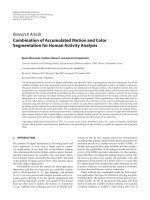
Definition 4. A nonsymmetric half-plane is a region of the
form
{m ≥ 0, n ≥ 0}∪{m>0, n<0} or their rotations.
An NSHP filter will have an impulse response which is
nonzero only in a particular NSHP. Based on the region of
support R, there are eight possible classes of NSHP filters,
[6, 19]. However, all discussions in this paper are based only
on R +
⊕ class filter, and it should be noted that, the results
of this class of filter are also extended to other seven classes
of NSHP filters. Figures 2(a) and 2(b)show the +
⊕ NSHP
region and the 2D recursion using a +
⊕ NSHP Filter [6, 19].
This paper focuses on NSHP filters and stabilizing
unstable NSHP filters using PLSI polynomials. 2D NSHP
polynomial and its region of support are defined as
follows.
Definition 5. A2DNSHPpolynomialofdegreeN [17]is
given by
A(z
1,
z
2
) =
N
R+⊕
N
R+⊕
a
mn
z
m
1
z
n
2
,(2)
where, the region of support, R+
⊕={m ≥ 0, n ≥ 0}∪{m>
0, n<0
} [6, 10].
The transfer function of the NSHP filter is given by
H(z
1
, z
2
) =
B(z
1,
z
2
)
A(z
1
, z
2
)
=
N
R+
⊕
N
R+
⊕
b
mn
z
m
1
z
n
2
N
R+⊕
N
R+⊕
a
mn
z
m
1
z
n
2
. (3)
In NSHP filters, the output y(m, n) can be calculated
recursively using the 2D difference equation given as
follows:
y(m, n)
=
R+⊕
a
kl
x(m −k, n −l)
−
R+⊕−(0,0)
b
kl
y(m − k, n −l).
(4)
With these preliminaries, the succeeding section demon-
strates the basic concept of LSI polynomials and the proce-
dures to obtain LSI polynomials in one and two dimensions.
3. Basic Concept of Least Squares Inverse
Polynomials (LSI) in 1D and 2D
The basic concept of LSI technique and the general procedure
to form LSI polynomials in one and two-dimensions are the
core of this section. Indeed in 2D, LSI is commonly known as
PLSI.
Let T
2
to be the distinguished boundary of the bicircle
defined by [(z
1
, z
2
); |z
1
|=1, |z
2
|=1] and U
2
to be the
closed region given by [(z
1
, z
2
); |z
1
|≤1, |z
2
|≤1].
Definition 6. If A(z)
=
N
n=0
a
n
z
n
is a given 1D polynomial
of degree N, then the 1D polynomial A
(z) =
M
m
=0
a
m
z
m
of
degree M, forms the LSI of A(z), if
A
(z) ≈
1
A(z)
for
|z|=1. (5)
In order to obtain the LSI, A
(z) let it be formed that
C(z)
= A(z) × A
(z) ≈ 1, (6)
and then form an error function E from C(z), such that
E
= (1 −c
0
)
2
+
j>0
c
2
j
. (7)
To evaluate the coefficients a
m
’s of the LSI polynomial A
(z),
minimize the error function E givenin(7)withrespectto
each a
m
to have the following linear system of equations:
∂E
∂a
m
= 0. (8)
4 EURASIP Journal on Advances in Signal Processing
R++
n
m
(a)
Output
mask
n
m
•
Present output y(m, n)
(b)
Figure 1: (a) The ++ Quarter-Plane. (b) 2D recursion Using ++ Filter.
R +
n
m
(a)
Output
mask
n
m
•
Present output
(b)
Figure 2: (a) The +⊕Nonsymmetric Half-Plane. (b) 2D recursion using a +⊕ Filter.
This will finally result in a set of linear algebraic equations
(also known as normal equations) which is given in the form
of matrix as follows:
T a
= a,(9)
where
T is a square symmetric positive definite matrix
(symmetric Toeplitz matrix) whose entries are functions of
a
n
’s where a
is a column vector of a
m
coefficients, and a is
a column vector whose first entry is a
0
and the rest of a
n
’s
are zeros. The solution of (9)willgivealla
m
coefficients
and, hence, the LSI polynomial, A
(z) which approximates
1/A(z).
Expert literature demonstrates that, the 1D LSI polyno-
mial, A
(z) corresponding to the unstable polynomial, A(z)
which is devoid of zeros on the unit circle is always stable
[11, 20]. This LSI method has been widely used to stabilize
unstable 1D recursive filters.
The procedure to obtain the PLSI polynomial corre-
sponding to a 2D NSHP polynomial is explored herewith.
Definition 7. If A(z
1
, z
2
) =
N
R+⊕
N
R+⊕
a
mn
z
m
1
z
n
2
is a 2D
NSHP polynomial of degree N in both variables, then the
2D polynomial A
(z
1
, z
2
) =
M
R+
⊕
M
R+
⊕
a
mn
z
m
1
z
n
2
of degree
M, forms the PLSI of A(z
1
, z
2
)if
A
(z
1
, z
2
) ≈
1
A(z
1
, z
2
)
for T
2
, (10)
(see [10]). To obtain A
(z
1
, z
2
)justlikein1D,firstform
C(z
1
, z
2
) = A(z
1
, z
2
) × A
(z
1
, z
2
) ≈ 1,
(11)
C(z
1,
z
2
) =
M+N
m=0
M+N
n=0
c
mn
z
m
1
z
n
2
≈ 1
. (12)
The approximation is achieved by choosing the coefficients
of
(z
1
, z
2
), such that the error energy “E” is minimized,
EURASIP Journal on Advances in Signal Processing 5
where,
E
= (1−c
00
)
2
+
M+N
m=0
M+N
n=0
c
mn
. (13)
Then differentiate E with respect to each unknown coeffi-
cient a
mn
as follows:
∂E
∂a
mn
. (14)
This will result in a set of linear algebraic equations of the
form
T a
= a. (15)
In (15),
T is a square symmetric Toeplitz matrix whose entries
are functions of a
mn
’s, a
is a column vector of a
mn
coefficients
as below:
a
={a
00
, a
01
, a
02
, , a
mn
}
t
, (16)
and
a is also a column vector like
a ={a
00
,0,0, ,0}
t
. (17)
The solution of (15)willgivealla
mn
coefficients and hence
the PLSI, A
(z
1
, z
2
) which approximates 1/A(z
1
, z
2
)[10].
In 1D, obtaining LSI polynomial is simple, but, it is
demonstrated in [21] that obtaining PLSI directly from the
2D polynomial is ext remely cumbersome, especially forming
T matrix in the normal equation (15).
The concept of form-preserving transformation [20, 21]
is commonly employed to convert the 2D problem into 1D
problem and therefore the stability of 2D is related to the
stability of 1D LSI. Once it is converted to a 1D problem,
the whole process of stabilization and stability testing is
simple. This justifies the choice of going for form-preserving
transformation. This paper compares the computations
involved in obtaining the PLSI using the existing form-
preserving transformation reported in [10] and the one used
in this paper.
The following section, introduces the new way of form-
preserving transformation that can be used to obtain the
PLSI in a simple manner. Based on this transformation, some
theorems have been proposed.
4. Form-Preserving Transformation and
Stability of PLSI Polynomials
The literature on the concept of form-preserving transfor-
mation is used in different contexts for first quadrant and
NSHP recursive digital filters. For instance, Shanks [22]
writes on techniques to design stable two-dimensional recur-
sive filters. He demonstrates that, one-dimensional filters
can be converted into two-dimensional filters with arbitrary
directivity in a two-dimensional frequency response plane.
In Shanks paper, and in subsequent ones [15, 23], the entire
discussions focus on “one-quadrant” or quarter-plane recur-
sive filters only. In [10], the concept of form-preserving
transform was used in the stabilization of 2D NSHP recursive
filters.
The PLSI method of stabilizing NSHP recursive filters
reported in [10] has the following shortcomings:
(i) the obtained LSI is always suboptimal;
(ii) computational complexity is obvious.
In [10] to obtain the PLSI polynomial, the form-preserving
transformation, A
(z
L
, z)whereL = 4N + 1 is applied. This
always leads to suboptimal (or constrained) polynomials and
does not guarantee stability. A suboptimal polynomial is not
always stable though it is reported in [10]as“always stable.”
This is a serious error. Unfortunately the authors of [10]
have overlooked the fact that the 1D LSI polynomial B(z)
generated by the form preserving transformation is lacunary
(missing some powers of z or some powers of z are forced
to have zero coefficients). Hence the stability of such 1D LSI
polynomials cannot be guaranteed though in some cases one
may get stable polynomial in spite of the constraints. So the
form preserving transformation reported in [10]isnolonger
applicable in the procedure for getting an always stable PLSI.
More details about suboptimal and lacunary polynomials are
reported in [24]. Moreover the computational complexity
involved in finding the autocorrelation coefficients and in
testing the suboptimal polynomials for stability is very high
in [10].
To overcome these shortcomings, the present work,
demonstrates a new way of form-preserving transformation
concerning NSHP, to convert the 2D NSHP polynomial into
1D polynomial. The emphasis here is that the presented
transformation when applied to NSHP will lead to optimal
LSI. If one attempts to use this transformation for first-
quadrant polynomial, this transformation will result in
suboptimal LSI and, hence, results into unstable PLSI.
Although QP filters form a subset of the more general
NSHP filters, the stability requirement for NSHP and QP are
different. A comparison on the stability of 2D QP and NSHP
PLSI polynomials can be found in [5].
This section, demonstrates a new way of form-preserving
transformation concerning NSHP polynomials, which will
be used to obtain the PLSI polynomial that correspond to the
given unstable 2D NSHP polynomials in a simple manner.
As mentioned earlier, PLSI method is used to stabilize
the unstable 2D NSHP polynomial corresponding to the
2D NSHP filter. Some definitions and theorems have been
introduced related to it.
Definition 8. ApolynomialA
F
(z) =
N
k
=0
a
k
z
k
is a form-
preserving 1D polynomial with respect to a 2D polynomial
6 EURASIP Journal on Advances in Signal Processing
A(z
1
, z
2
) =
M
R+
⊕
M
R+
⊕
a
mn
z
m
1
z
n
2
if for every integer set (m, n)
in A(z
1
, z
2
) there exists a unique k in A
F
(z) such that a
k
=
a
mn
.
Definition 9. Given a finite length discrete sequence of the
form
{a
0
, a
1
, a
2
, , a
k
}. The autocorrelation coefficients γ
i
’s
of the sequence is defined as γ
i
=
k
j=0
a
j
a
j+i
,wherei =
0, 1,2, , k,(see[25]).
This leads to introduce the following new theorem.
Theorem 1. If A(z
1
, z
2
) =
N
R+⊕
N
R+⊕
a
mn
z
m
1
z
n
2
is a 2D
NSHP polynomial of degree N, then its form-preserving 1D
polynomial A
F
(z) = A(z
1
z
2
)|
z
1
=z
L
z
2=z
, when L = 2N +1,will
be nonlacuncary, and it will have the same autocorrelation
coefficie nts as the polynomial A(z
1
, z
2
).
Proof. For A
F
(z) to be a form-preserving 1D polynomial
with respect to a 2D NSHP polynomial, A(z
1
, z
2
) the number
of distinct terms in these two polynomials should be the
same. Let the 2D NSHP polynomial be of degree N.
From the nature of NSHP polynomials, the number of
distinct terms in A
F
(z)isNL+2N + 1. Similarly, the number
of distinct terms in A(z
1
, z
2
) = (N + 1)(2N + 1). To find the
value of L, equate the number of terms in A
F
(z)andA(z
1
, z
2
):
NL+2N +1
= (N + 1)(2N +1),
NL+2N +1
= 2NN +2N + N +1
NL
= 2NN + N
L
= 2N +1
(18)
Thus the proof.
Let A(z
1
, z
2
) =
1
R+⊕
1
R+⊕
a
mn
z
m
1
z
n
2
be a 2D NSHP
polynomial of first degree.This2DNSHPpolynomialcanbe
written as follows:
A(z
1
, z
2
) = a
00
+ a
01
z
2
+ a
10
z
1
+ a
11
z
1
z
2
+a
1−1
z
1
z
−1
2
. (19)
This imply to obtain the form-preserving 1D polynomial
A
F
(z)of(19) with the form-preserving transformation
A(z
1
, z
2
)|
z
1
=z
L
z
2=z
, when L = 2N +1asfollows:
A
F
(z) = A(z
2N+1
, z) = A(z
3
z),
A
F
(z) = a
00
+ a
01
z + a
10
z
3
+ a
11
z
4
+a
1−1
z
2
.
(20)
Equation (20)canberewrittenasbelow:
A
F
(z) = a
00
+ a
01
z+a
1−1
z
2
+ a
10
z
3
+ a
11
z
4
. (21)
From (19)and(21), it is evident that the number of
distinct terms in the 2D polynomial A(z
1
, z
2
) is the same
as the number of distinct terms in the form-preserving
1D polynomial A
F
(z) and in view of Theorem 1, the
autocorrelation coefficients γ
i
’s of (19)and(21) are the same.
Theyareasfollows:
a
2
00
+ a
2
01
+ a
2
1
−1
+ a
2
10
+ a
2
11
= γ
0
,
a
00
a
01
+ a
01
a
1−1
+ a
1−1
a
10
+ a
10
a
11
= γ
1
,
a
00
a
1−1
+ a
01
a
10
+ a
10
a
1−1
= γ
2
,
a
00
a
10
+ a
01
a
11
= γ
3
,
a
00
a
11
= γ
4
.
(22)
Obviously from (21) the form-preserving 1D polynomial
obtained from A(z
1
, z
2
)withL = (2N +1)isnonlacunary
(i.e., no missing powers of z). Therefore any positive integer
value of L>(2N + 1) will also result in form-preserving 1D
polynomial, having the same autocorrelation coefficients as
that of the given 2D polynomial, but the resulting 1D form-
preserving polynomial will be definitely lacunary.
Before discussing the existing theorems related to sta-
bility, it is important to discover the relationship between
stability and causality.
Stability does not include causality and anticausality. A
causal system is stable, when all its poles lie inside the unit
circle, the zeros are irrelevant. Likewise an anticausal system
is stable, when all its poles lie outside the unit circle, again the
zeros are irrelevant. Those systems that have poles right on
the unit circle or called marginally stable. Causality is often
a desirable constraint to impose in designing 1D systems. An
anticausal system would require delay, which is undesirable
in such applications as real-time speech processing. In typical
2D signal processing applications such as image processing,
causality has little importance. At any given time, a complete
frame of an image may be available for processing, and it may
be processed from left to right, from top to bottom, or in any
direction one chooses.
At this point, this paper defines the existing theorems
related to stability in which 1D and 2D Z-transforms are
defined with positive powers of Z.
Theorem 2. Given a t ransfer function of certain 1D LSI
system, H(z)
= 1/A(z).ApolynomialA(z) is stable if and only
if
A(z)
/
=0, |z|≤1, (23)
(see [18]). The condition as in (23) states that a 1D polynomial
is stable, if and only if, a ll its zeros lie outside the unit circle.
Theorem 3. Given a transfer function of some 2D LSI system,
H(z
1
, z
2
) = 1/A(z
1
, z
2
).ApolynomialA(z
1
, z
2
) is stable if and
only if
A(z
1
, z
2
)
/
=0, for U
2
, (24)
(see [18]).
Theorem 4. If A
(z
1
, z
2
) is a PLSI polynomial of A(z
1
, z
2
),
then A
F
(z) is the LSI polynomial of A
F
(z).
EURASIP Journal on Advances in Signal Processing 7
Proof. The proof of this theorem derives from the definitions,
and the method of obtaining PLSI polynomials discussed in
Section 3. Initially, it is assumed that A
(z
1
, z
2
)isaPLSIof
A(z
1
, z
2
).The2DpolynomialC(z
1
, z
2
)asgivenin(12), and
its form-preserving 1D polynomial C
F
(z) will have the same
coefficients. Therefore, the error function E in (13)willbe
the same for both polynomials, and that results in the same
set of linear equations
T a
= a as given in (15) and hence the
coefficients of the polynomial A
F
(z) will turn out to be the
same as those of A
(z
1
, z
2
). Hence A
F
(z) is the LSI of A
F
(z).
TheconverseofTheorem 4 is also true.
This paper now introduces a new stability theorem.
Theorems 1 and 4 are the basis for Theorem 5.
Theorem 5. A 2D NSHP, PLSI polynomial A
(z
1
, z
2
) =
N
R+
⊕
N
R+
⊕
a
mn
z
m
1
z
n
2
of degree N, is stable, if and only if, the
1D form-preserving polynomial A
F
(z) obtained using the form-
preserving transformation, A
(z
2N+1
, z) is stable.
Proof. The necessary and sufficient conditions for A
(z
1
, z
2
)
to be stable is that [6]
(i) A
(z, z)
/
=0 when |z|≤1;
(ii) A
(z
1
, z
2
)
/
=0onT
2
.
(25a)
The new set of stability conditions equivalent to (25a)by
applying homomorphic transformation [26] is stated as
follows:
(i) A
(z
l
1
, z
l
2
)
/
=0 when |z|≤1;
(ii) A
(z
1
, z
2
)
/
=0onT
2
.
(25b)
For some l
1
, l
2
∈ z
+
,wherez
+
denotes the positive integers
[26]. It has been shown in [20] that the PLSI polynomial
A
(z
1
, z
2
)ofany2DpolynomialA(z
1
, z
2
)devoidonT
2
itself. This satisfies the condition (ii) of (25b). Now we have
to show that the condition (i) of (25b) is fullfilled. From
Theorem 4, A
F
(z) is the LSI of A
F
(z), and from Theorem 1,
A
F
(z), which is obtained with the form-preserving transfor-
mation z
1
= z
L
, z
2
= z when L = 2N+1 has the same number
oftermsasinA
(z
1
, z
2
), and the autocorrelation coefficients
of both A
F
(z)andA
(z
1
, z
2
) are the same. Obviously, only
with this form-preserving transformation, the resulting 1-D
LSI polynomial A
F
(z) is nonlacunary, and optimal while 1D
LSI polynomial resulting from L>2N + 1 will definitely be
lacunary, and suboptimal. It is an established fact that the
optimal 1D LSI polynomial A
F
(z) is stable [25]. The form-
preserving 1D polynomial, A
F
(z) = A
(z
l
1
, z
l
2
)|
l
1
=2N+1
l
2
=1
is thus
stable. Therefore, condition (i) of (25b) is also fulfilled. So,
the PLSI polynomial A
(z
1
, z
2
) is stable. This demonstrates
Theorem 5.
In the process of forming the PLSI polynomial cor-
responding to the given 2D NSHP polynomial, form-
preserving transformation is used to convert the 2D NSHP
polynomial into 1D and, then, obtain the 1D LSI of the form-
preserving 1D polynomial. The PLSI can then be formed
from 1D LSI.
From Theorems 4 and 5, it is obvious that, to prove PLSI
polynomial A
(z
1
, z
2
) is stable, it is enough to demonstrate
its form-preserving 1D polynomial, A
F
(z) with the transfor-
mation, A
(z
2N+1
, z) is stable.
5. Numerical Examples
This section, focuses on some numerical examples for
stabilizing 2D NSHP polynomials of first and second degree.
The proposed theorems and procedures are applied to form
the PLSI polynomials in the examples provided by the
literature [10], and demonstrate that, the proposed theorems
andproceduresstillresultinastablePLSIpolynomialas
with the existing method in the literature, but with reduced
complexity.
Example 1 (Polynomial of first degree). Consider the follow-
ing 2D NSHP polynomial of first degree:
A(z
1
, z
2
) = 0.9z
1
z
−1
2
+0.3+0.6z
2
+0.6z
1
+0.8z
1
z
2
, (26)
(see [10]). The form-preserving 1D polynomial A
F
(z)of
A(z
1
, z
2
) is obtained using the new way of form-preserving
transformation (from Theorem 1)
A
F
(z) = A(z
2N+1
, z) = A(z
3
z) (since N = 1). (27)
Thus,
A
F
(z) = 0.8z
4
+0.6z
3
+0.9z
2
+0.6z +0.3. (28)
The roots of A
F
(z) are 0.9393, 0.9393, 0.6520, and 0.6520.
From Theorem 2, therefore, the form-preserving 1D poly-
nomial is unstable. Theorem 4 is applied to form the LSI
polynomial of A
F
(z). The LSI of A
F
(z)isA
F
(z)andto
find out A
F
(z), the autocorrelation coefficients of A
F
(z)are
computed as follows:
γ
0
=2.26, γ
1
=1.74, γ
2
=1.35, γ
3
=0.66, γ
4
=0.24.
(29)
Now the normal equation is formed (15) as follows:
⎡
⎢
⎢
⎢
⎢
⎢
⎢
⎢
⎢
⎢
⎣
2.26 1.74 1.35 0.66 0.24
1.74 2.26 1.74 1.35 0.66
1.35 1.74 2.26 1.74 1.35
0.66 1.35 1.74 2.26 1.74
0.24 0.66 1.35 1.74 2.26
⎤
⎥
⎥
⎥
⎥
⎥
⎥
⎥
⎥
⎥
⎦
×
⎡
⎢
⎢
⎢
⎢
⎢
⎢
⎢
⎢
⎢
⎢
⎣
a
00
a
01
a
1−1
a
10
a
11
⎤
⎥
⎥
⎥
⎥
⎥
⎥
⎥
⎥
⎥
⎥
⎦
=
⎡
⎢
⎢
⎢
⎢
⎢
⎢
⎢
⎢
⎢
⎣
0.3
0
0
0
0
⎤
⎥
⎥
⎥
⎥
⎥
⎥
⎥
⎥
⎥
⎦
, (30)
8 EURASIP Journal on Advances in Signal Processing
⎡
⎢
⎢
⎢
⎢
⎢
⎢
⎢
⎢
⎢
⎢
⎣
a
00
a
01
a
1−1
a
10
a
11
⎤
⎥
⎥
⎥
⎥
⎥
⎥
⎥
⎥
⎥
⎥
⎦
=
⎡
⎢
⎢
⎢
⎢
⎢
⎢
⎢
⎢
⎢
⎣
2.26 1.74 1.35 0.66 0.24
1.74 2.26 1.74 1.35 0.66
1.35 1.74 2.26 1.74 1.35
0.66 1.35 1.74 2.26 1.74
0.24 0.66 1.35 1.74 2.26
⎤
⎥
⎥
⎥
⎥
⎥
⎥
⎥
⎥
⎥
⎦
−1
×
⎡
⎢
⎢
⎢
⎢
⎢
⎢
⎢
⎢
⎢
⎣
0.3
0
0
0
0
⎤
⎥
⎥
⎥
⎥
⎥
⎥
⎥
⎥
⎥
⎦
, (31)
⎡
⎢
⎢
⎢
⎢
⎢
⎢
⎢
⎢
⎢
⎢
⎣
a
00
a
01
a
1−1
a
10
a
11
⎤
⎥
⎥
⎥
⎥
⎥
⎥
⎥
⎥
⎥
⎥
⎦
=
⎡
⎢
⎢
⎢
⎢
⎢
⎢
⎢
⎢
⎢
⎣
0.3964
−0.3078
−0.1282
0.1744
−0.0100
⎤
⎥
⎥
⎥
⎥
⎥
⎥
⎥
⎥
⎥
⎦
, (32)
A
F
(z)=0.3964 −0.3078z −0.1282z
2
+0.1744z
3
−0.0100z
4
.
(33)
The roots of A
F
are 16.5625, 1.4479, 1.2857, and 1.2857.
From Theorem 2, therefore the 1D LSI polynomial A
F
(z)
corresponding to A
F
(z) is stable. It is interesting that,
even though 2D to 1D transformations in general are
irreversible (i.e., singular) in the case of form-preserving
transformations, there exists a one-to-one mapping among
the coefficients of the 2D, and the transformed 1D polynomi-
als, and the 2D polynomials can be constructed exactly from
the 1D polynomial. Thus, the 2D PLSI corresponding to the
1D LSI (33)readsasfollows:
A
(z
1
, z
2
) = 0.3964 − 0.3078z
2
+0.1744z
1
−0.0100z
1
z
2
−0.1282z
1
z
−1
2
.
(34)
ThePLSIpolynomialdemonstratedin(34) is stable in view
of Theorem 5. This is in line with the result reported in
[10].
Example 2 (Polynomial of second degree). Consider the
following 2D NSHP polynomial of second degree:
A(z
1
, z
2
) = 0.6+0.9z
2
+0.3z
2
2
+0.9z
1
+1.5z
1
z
2
+0.9z
1
z
2
2
+0.3z
2
1
+0.9z
2
1
z
2
+0.6z
2
1
z
2
2
+0.5z
1
z
−1
2
+0.8z
2
1
z
−1
2
+0.7z
1
z
−2
2
+ z
2
1
z
−2
2
,
(35)
(see [10]). The form-preserving 1D polynomial A
F
(z)of
A(z
1
, z
2
) is obtained using the new way of form-preserving
transformation (from Theorem 1):
A
F
(z) = A(z
2N+1
, z) = A(z
5
, z) (since N = 2),
A
F
(z) = 0.6+0.9z +0.3z
2
+0.9z
5
+1.5z
6
+0.9z
7
+0.3z
10
+0.9z
11
+0.6z
12
+0.5z
4
+0.8z
9
+0.7z
3
+ z
8
.
(36)
This can be read as follows:
A
F
(z) = 0.6+0.9z +0.3z
2
+0.7z
3
+0.5z
4
+0.9z
5
+1.5z
6
+0.9z
7
+ z
8
+0.8z
9
+0.3z
10
+0.9z
11
+0.6z
12
.
(37)
The roots of A
F
(z) are 1.0728, 1.0728, 0.9481, 0.9481,
1.0021, 1.0021, 0.9545, 0.9545, 1.3298, 1.0892, 1.0892, and
0.6697. From Theorem 2, therefore, the form-preserving 1D
polynomial is unstable. Theorem 4 is applied to form the
LSI polynomial of A
F
(z). The LSI of A
F
(z)isA
F
(z)andto
find out A
F
(z), the autocorrelation coefficients of A
F
(z)are
computed as follows: γ
0
= 8.77, γ
1
= 7.27, γ
2
= 6.57,
γ
3
= 6.39, γ
4
= 5.27, γ
5
= 5.42, γ
6
= 4.43, γ
7
= 2.88,
γ
8
= 2.34, γ
9
= 1.44, γ
10
= 1.17, γ
11
= 1.08, γ
12
= 0.36.
Now form the normal equation (15) as follows:
⎡
⎢
⎢
⎢
⎢
⎢
⎢
⎢
⎢
⎢
⎢
⎢
⎢
⎢
⎢
⎢
⎢
⎢
⎢
⎢
⎢
⎢
⎢
⎢
⎢
⎢
⎢
⎢
⎢
⎢
⎢
⎢
⎢
⎢
⎢
⎣
8.77 7.27 6.57 6.39 5.27 5.42 4.43 2.88 2.34 1.44 1.17 1.08 0.36
7.27 8.77 7.27 6.57 6.39 5.27 5.42 4.43 2.88 2.34 1.44 1.17 1.08
6.57 7.27 8.77 7.27 6.57 6.39 5.27 5.42 4.43 2.88 2.34 1.44 1.17
6.39 6.57 7.27 8.77 7.27 6.57 6.39 5.27 5.42 4.
43 2.88 2.34 1.44
5.27 6.39 6.57 7.27 8.77 7.27 6.57 6.39 5.27 5.42 4.43 2.88 2.34
5.42 5.27 6.39 6.57 7.27 8.77 7.27 6.57 6.39 5.27 5.42 4.43 2.88
4.43 5.42 5.27 6.39 6.57 7.27 8.77 7.27 6.57 6.39 5.27 5.42 4.43
2.88 4.43 5.42 5.27 6.39 6.57 7
.27 8.77 7.27 6.57 6.39 5.27 5.42
2.34 2.88 4.43 5.42 5.27 6.39 6.57 7.27 8.77 7.27 6.57 6.39 5.27
1.44 2.34 2.88 4.43 5.42 5.27 6.39 6.57 7.27 8.77 7.27 6.57 6.39
1.17 1.44 2.34 2.88 4.43 5.42 5.27 6.39 6.57 7.27 8.77 7.27 6.57
1.08 1.17 1.
44 2.34 2.88 4.43 5.42 5.27 6.39 6.57 7.27 8.77 7.27
0.36 1.08 1.17 1.14 2.34 2.88 4.43 5.42 5.27 6.39 6.57 7.27 8.77
⎤
⎥
⎥
⎥
⎥
⎥
⎥
⎥
⎥
⎥
⎥
⎥
⎥
⎥
⎥
⎥
⎥
⎥
⎥
⎥
⎥
⎥
⎥
⎥
⎥
⎥
⎥
⎥
⎥
⎥
⎥
⎥
⎥
⎥
⎥
⎦
×
⎡
⎢
⎢
⎢
⎢
⎢
⎢
⎢
⎢
⎢
⎢
⎢
⎢
⎢
⎢
⎢
⎢
⎢
⎢
⎢
⎢
⎢
⎢
⎢
⎢
⎢
⎢
⎢
⎢
⎢
⎢
⎢
⎢
⎢
⎢
⎢
⎢
⎢
⎢
⎢
⎣
a
00
a
01
a
02
a
1−2
a
1−1
a
10
a
11
a
12
a
2−2
a
2−1
a
20
a
21
a
22
⎤
⎥
⎥
⎥
⎥
⎥
⎥
⎥
⎥
⎥
⎥
⎥
⎥
⎥
⎥
⎥
⎥
⎥
⎥
⎥
⎥
⎥
⎥
⎥
⎥
⎥
⎥
⎥
⎥
⎥
⎥
⎥
⎥
⎥
⎥
⎥
⎥
⎥
⎥
⎥
⎦
=
⎡
⎢
⎢
⎢
⎢
⎢
⎢
⎢
⎢
⎢
⎢
⎢
⎢
⎢
⎢
⎢
⎢
⎢
⎢
⎢
⎢
⎢
⎢
⎢
⎢
⎢
⎢
⎢
⎢
⎢
⎢
⎢
⎢
⎢
⎢
⎣
0.6
0
0
0
0
0
0
0
0
0
0
0
0
⎤
⎥
⎥
⎥
⎥
⎥
⎥
⎥
⎥
⎥
⎥
⎥
⎥
⎥
⎥
⎥
⎥
⎥
⎥
⎥
⎥
⎥
⎥
⎥
⎥
⎥
⎥
⎥
⎥
⎥
⎥
⎥
⎥
⎥
⎥
⎦
. (38)
EURASIP Journal on Advances in Signal Processing 9
Solving (38)weget,
⎡
⎢
⎢
⎢
⎢
⎢
⎢
⎢
⎢
⎢
⎢
⎢
⎢
⎢
⎢
⎢
⎢
⎢
⎢
⎢
⎢
⎢
⎢
⎢
⎢
⎢
⎢
⎢
⎢
⎢
⎢
⎢
⎢
⎢
⎢
⎢
⎢
⎢
⎢
⎢
⎣
a
00
a
01
a
02
a
1−2
a
1−1
a
10
a
11
a
12
a
2−2
a
2−1
a
20
a
21
a
22
⎤
⎥
⎥
⎥
⎥
⎥
⎥
⎥
⎥
⎥
⎥
⎥
⎥
⎥
⎥
⎥
⎥
⎥
⎥
⎥
⎥
⎥
⎥
⎥
⎥
⎥
⎥
⎥
⎥
⎥
⎥
⎥
⎥
⎥
⎥
⎥
⎥
⎥
⎥
⎥
⎦
=
⎡
⎢
⎢
⎢
⎢
⎢
⎢
⎢
⎢
⎢
⎢
⎢
⎢
⎢
⎢
⎢
⎢
⎢
⎢
⎢
⎢
⎢
⎢
⎢
⎢
⎢
⎢
⎢
⎢
⎢
⎢
⎢
⎢
⎢
⎢
⎣
0.4231
−0.3344
0.0815
−0.2717
0.2325
−0.3339
0.1882
−0.0001
0.1563
−0.0342
0.0167
−0.0488
−0.0309
⎤
⎥
⎥
⎥
⎥
⎥
⎥
⎥
⎥
⎥
⎥
⎥
⎥
⎥
⎥
⎥
⎥
⎥
⎥
⎥
⎥
⎥
⎥
⎥
⎥
⎥
⎥
⎥
⎥
⎥
⎥
⎥
⎥
⎥
⎥
⎦
. (39)
Now, the PLSI A
F
(z)is
A
F
(z) = 0.4231 − 0.3344z +0.0815z
2
−0.2717z
3
+0.2325z
4
−0.3339z
5
+0.1882z
6
−0.0001z
7
+0.1563z
8
−0.0342z
9
+0.0167z
10
−0.0488z
11
−0.0309z
12
.
(40)
The roots of A
F
(z) are as follows: 2.4606, 1.1771, 1.1771,
1.1854, 1.1854, 1.4025, 1.4025, 1.0727, 1.0727, 1.0782,
1.0782, and 1.0863. From Theorem 2, therefore, 1D LSI
polynomial A
F
(z) corresponding to A
F
(z) is stable. The 2D
PLSI obtained from LSI (40) is as follows:
A
(z
1
, z
2
) = 0.4231 − 0.3344z
2
+0.0815z
2
2
−0.3339z
1
+0.1882z
1
z
2
−0.0001z
1
z
2
2
+0.0167z
2
1
−0.0488z
2
1
z
2
−0.0309z
2
1
z
2
2
+0.2325z
1
z
−1
2
−0.0342z
2
1
z
−1
2
−0.2717z
1
z
−2
2
+0.1563z
2
1
z
−2
2
.
(41)
The PLSI polynomial given in (41)isstableinviewof
Theorem 5. This result is also in line with the results reported
in [10].
Example 3 (Polynomial of first degree). Consider the follow-
ing 2D NSHP polynomial of first degree (random example):
A(z
1
, z
2
) = 0.2z
1
z
−1
2
+0.1+0.7z
2
+0.9z
1
+0.4z
1
z
2
. (42)
The form-preserving 1D polynomial A
F
(z)ofA(z
1
, z
2
)is
obtained using the new way of form-preserving transforma-
tion (from Theorem 1):
A
F
(z) = A(z
2N+1
, z) = A(z
3
, z) (since N = 1). (43)
Thus,
A
F
(z) = 0.4z
4
+0.9z
3
+0.2z
2
+0.7z +0.1. (44)
The roots of A
F
(z) are 2.3369, 0.8584, 0.8584, and 0.1452.
From Theorem 2, therefore, the form-preserving 1D polyno-
mial is unstable. The LSI of A
F
(z)isA
F
(z)andtofindout
A
F
(z), the autocorrelation coefficients of A
F
(z)arecomputed
as follows:
γ
0
=1.51, γ
1
=0.75, γ
2
=0.73, γ
3
=0.37, γ
4
=0.04.
(45)
Now form the normal equation (15) as follows:
⎡
⎢
⎢
⎢
⎢
⎢
⎢
⎢
⎢
⎢
⎣
1.51 0.75 0.73 0.37 0.04
0.75 1.51 0.75 0.73 0.37
0.73 0.75 1.51 0.75 0.73
0.37 0.73 0.75 1.51 0.75
0.04 0.37 0.73 0.75 1.51
⎤
⎥
⎥
⎥
⎥
⎥
⎥
⎥
⎥
⎥
⎦
×
⎡
⎢
⎢
⎢
⎢
⎢
⎢
⎢
⎢
⎢
⎢
⎣
a
00
a
01
a
1−1
a
10
a
11
⎤
⎥
⎥
⎥
⎥
⎥
⎥
⎥
⎥
⎥
⎥
⎦
=
⎡
⎢
⎢
⎢
⎢
⎢
⎢
⎢
⎢
⎢
⎣
0.1
0
0
0
0
⎤
⎥
⎥
⎥
⎥
⎥
⎥
⎥
⎥
⎥
⎦
, (46)
⎡
⎢
⎢
⎢
⎢
⎢
⎢
⎢
⎢
⎢
⎢
⎣
a
00
a
01
a
1−1
a
10
a
11
⎤
⎥
⎥
⎥
⎥
⎥
⎥
⎥
⎥
⎥
⎥
⎦
=
⎡
⎢
⎢
⎢
⎢
⎢
⎢
⎢
⎢
⎢
⎣
1.51 0.75 0.73 0.37 0.04
0.75 1.51 0.75 0.73 0.37
0.73 0.75 1.51 0.75 0.73
0.37 0.73 0.75 1.51 0.75
0.04 0.37 0.73 0.75 1.51
⎤
⎥
⎥
⎥
⎥
⎥
⎥
⎥
⎥
⎥
⎦
−1
×
⎡
⎢
⎢
⎢
⎢
⎢
⎢
⎢
⎢
⎢
⎣
0.1
0
0
0
0
⎤
⎥
⎥
⎥
⎥
⎥
⎥
⎥
⎥
⎥
⎦
, (47)
⎡
⎢
⎢
⎢
⎢
⎢
⎢
⎢
⎢
⎢
⎢
⎣
a
00
a
01
a
1−1
a
10
a
11
⎤
⎥
⎥
⎥
⎥
⎥
⎥
⎥
⎥
⎥
⎥
⎦
=
⎡
⎢
⎢
⎢
⎢
⎢
⎢
⎢
⎢
⎢
⎣
0.1065
−0.0368
−0.0476
0.0011
0.0287
⎤
⎥
⎥
⎥
⎥
⎥
⎥
⎥
⎥
⎥
⎦
, (48)
A
F
(z) = 0.1065 − 0.0368z − 0.0476z
2
+0.0011z
3
+0.0287z
4
.
(49)
The roots of A
F
(z) are 1.4952, 1.4952, 1.2884, and 1.2884.
From Theorem 2, therefore, 1D LSI polynomial A
F
(z)corre-
sponding to A
F
(z) is stable. Then, the 2D PLSI is obtained in
relationship to the 1D LSI of (49) as follows:
A
(z
1
, z
2
) = 0.1065 − 0.0368z
2
+0.0011z
1
−0.0287z
1
z
2
−0.0476z
1
z
−1
2
.
(50)
The PLSI polynomial given in (50)isstableinviewof
Theorem 5.
It is evident, from the above three numerical examples,
discussed in this section that, the PLSI polynomial obtained
with the new way of form-preserving transformation always
results in a stable system.
10 EURASIP Journal on Advances in Signal Processing
6. Lagrange Multiplier Method for
Testing Stability
In all the three numerical examples discussed, in the
preceding section, the stability of the form-preserving 1D LSI
was tested using root finding method. The stability of only
first-, and second-degree LSI polynomials was dealt with. In
order to generalize the validity for any degree, a theoretical
method of testing the stability of the form-preserving ID LSI
based on Lagrange Multipliers Method is introduced.
It is well known that, in the process of forming LSI
polynomial, the minimum error E as in (7)isE
= 1 −
a
0
a
0
,wherea
0
and a
0
are the constant terms in the original
unstable polynomial, and LSI polynomial, respectively, [10,
11]. It is demonstrated in [27] that, for a polynomial of
degree N there are in total 2
N
polynomials, including the
given polynomial, which will have the same autocorrelation
coefficients as the given polynomial and hence the same
magnitude spectra, and out of which, only one polynomial
is stable for which the constant term is highest in order to
achieve minimum error. Since A
F
(z) is the form-preserving
1D polynomial of A
(z
1
, z
2
), to demonstrate that the PLSI
polynomial A
(z
1
, z
2
) is stable, it is enough that the constant
term of the form-preserving 1D polynomial, A
F
(z) is the
highest. So we only test the 1D LSI A
F
(z) for stability.
Let A
F
(z) be the stable version of A
F
(z). In this method,
one has to maximize the function f as
f
= a
00
, (51)
satisfying the constraints g
i
given as
g
i
=
N
r=0
a
r
a
r+s
−γ
s
= 0, s = 0, 1,2, , N, (52)
where
γ
S
=
N
r=0
a
r
a
r+s
, s = 0, 1,2, , N. (53)
That is,
g
i
= 0, i = 0, 1,2, , N. (54)
Then, the Lagrange function is formed, L(a
00
, λ
j
) = f +
N
j=0
λ
j
g
j
,whereλ
j
’s are the Lagrange multipliers. Then
form
∂L(a
00
, λ
j
)
∂a
00
= 0
, (55)
∂L(a
00
, λ
j
)
∂λ
j
= 0, j = 0,1, 2, , N
. (56)
Equation (56) is called Lagrange equation.
In this method, if the number of unknowns (a
mn
’s and
λ
j
’s) is greater than the number of constraint equations (55)
and (56), then, the solution may exist for the set of equations
and the optimum can be obtained for its constant term a
00
.
If so, the form-preserving 1D LSI will be stable and hence the
PLSI. On the other hand, if the number of unknowns is less
than the number of constraint equations, the solution may
not exist, and optimum may not be obtained for its constant
term a
00
. In this case, the PLSI may be unstable.
In the computer-aided optimization method of solving
nonlinear equations, one will be assured of a real solution
if the total number of unknowns, namely, a
mn
’s and λ
j
’s
is greater than the number of equations by at least one.
Our interest in this section is in establishing theoretically the
fact that, an optimum solution exists for the set of nonlinear
equations in t he maximization process. This ensures the
stability of the LSI polynomial and hence PLSI polynomial.
On the other hand, if the number of unknowns is less than
the number of nonlinear equations, in the computer-aided
optimization, and since the programmer has no degree of
freedom, sometimes it may not give us any real solution at
all. If this is the case, the PLSI will not be stable.
If the nonlinear equations given in (55)and(56)are
solvable and if the solution with all λ
j
’s positive exists, then
the necessary condition for the existence of the optimum is
satisfied, and the real optimum for a
00
in the maximization
process using Lagrange multiplier method will be reached. If
so resulting LSI and PLSI polynomial will be definitely stable.
The following examples clearly illustrate the application
of Lagrange multiplier method in testing the stability of LSI
and hence PLSI polynomial.
Example 4 (Polynomial of first degree). Consider a 2D PLSI
polynomial of first degree:
A
(z
1
, z
2
) = a
00
+ a
01
z
2
+ a
10
z
1
+ a
11
z
1
z
2
+ a
1−1
z
1
z
−1
2
,
(57)
and test the stability of (57) applying the proposed and
existing methods.
New Method. The form-preserving 1D polynomial of
A
(z
1
, z
2
)in(57) with the proposed form-preserving trans-
formation A
F
(z) = A
(z
2N+1
z) = A
(z
3
z) (since N = 1) is as
follows:
A
F
(z) = a
00
+ a
01
z + a
1−1
z
2
+ a
10
z
3
+ a
11
z
4
. (58)
Let
A
F
(z) = a
00
+ a
01
z + a
1−1
z
2
+ a
10
z
3
+ a
11
z
4
(59)
be the stable version of polynomial A
F
(z). The autocorrela-
tion constraint equations of (59)areasfollows:
a
2
00
+ a
2
01
+ a
2
1
−1
+ a
2
10
+ a
2
11
= γ
0
,
a
00
a
01
+ a
01
a
1−1
+ a
1−1
a
10
+ a
10
a
11
= γ
1
,
a
00
a
1−1
+ a
01
a
10
+ a
10
a
1−1
= γ
2
,
a
00
a
10
+ a
01
a
11
= γ
3
,
a
00
a
11
= γ
4
.
(60)
EURASIP Journal on Advances in Signal Processing 11
This implies that, at the end of maximization process, five
autocorrelation constraint equations are reached as in (60),
and one Lagrange equation as in (56) totalling six nonlinear
equations. There are 5 a
mn
’s, and 5 λ
j
’s as unknowns,
totalling 10 unknowns, which can be easily solved, and the
optimum a
00
exists. Therefore, in this case the LSI as in (58)
andPLSIasin(57)willbedefinitely stable.
Existing Method. The form-preserving 1D polynomial of
A
(z
1
, z
2
) with the existing form-preserving transformation
[10] is as follows:
A
F
(z) = A
(z
4N+1
z) = A
(z
5
z)
, (61)
A
F
(z) = a
00
+ a
01
z+0 + 0 + a
1−1
z
4
+ a
10
z
5
+ a
11
z
6
. (62)
Let A
F
(z) be the stable version of (62). The autocorrelation
coefficients of (62)areasfollows:
a
2
00
+ a
2
01
+ a
2
1
−1
+ a
2
10
+ a
2
11
= γ
0
,
a
00
a
01
+ a
1−1
a
10
+ a
10
a
11
= γ
1
,
a
1−1
a
11
= γ
2
∗
,
a
01
a
1−1
= γ
3
∗
,
a
00
a
1−1
+ a
01
a
10
= γ
4
,
a
00
a
10
+ a
01
a
11
= γ
5
,
a
00
a
11
= γ
6
.
(63)
In (63),
∗ indicates the autocorrelation constraint equations
that do not contain a
00
.
The autocorrelation constraint equations given in (63)
are seven in number. It may be noted that, two of these
equations do not contain the constant coefficient a
00
. In this
example, the total number of nonlinear equations is eight
including the Lagrange equation. The total unknowns will be
5+5
= 10. In this, the number of λ
j
’s have been considered
as only five because λ
j
’s do not have to be assigned for the
nonlinear equations that do not contain a
00
. Thus, there are
10 unknowns and eight equations. With the existing method
also, the 1D LSI (62)PLSI(57) is found stable, but with the
new method proposed in this paper, the number of equations
is only six.
Example 5 (Polynomial of second degree).
New Method.LetA
(z
1
, z
2
) =
2
R+
⊕
2
R+
⊕
a
mn
z
m
1
z
n
2
be a
second-degree polynomial, which can be expanded as
A
(z
1
, z
2
) = a
00
+ a
01
z
2
+ a
02
z
2
2
+ a
10
z
1
+ a
11
z
1
z
2
+ a
12
z
1
z
2
2
+ a
20
z
2
1
+ a
21
z
2
1
z
2
+ a
22
z
2
1
z
2
2
+ a
1−1
z
1
z
−1
2
+ a
2−1
z
2
1
z
−1
2
+ a
1−2
z
1
z
−2
2
+ a
2−2
z
2
1
z
−2
2
.
(64)
The form-preserving 1D polynomial A
F
(z) obtained with
L
= 2N + 1, in the PLSI polynomial A
(z
1
, z
2
)is
A
F
(z) = A
(z
2N+1
, z) = A
(z
5
z) = a
00
+ a
01
z + a
02
z
2
+ a
10
z
5
+ a
11
z
6
+ a
12
z
7
+ a
20
z
10
+ a
21
z
11
+ a
22
z
12
+ a
1−1
z
4
+ a
2−1
z
9
+ a
1−2
z
3
+ a
2−2
z
8
.
(65)
This can be written as follows:
A
F
(z) = a
00
+ a
01
z + a
02
z
2
+ a
1−2
z
3
+ a
1−1
z
4
+ a
10
z
5
+ a
11
z
6
+ a
12
z
7
+ a
2−2
z
8
+ a
2−1
z
9
+ a
20
z
10
+ a
21
z
11
+ a
22
z
12
.
(66)
This paper uses Lagrange multiplier method as in Example 4,
to test whether the LSI, and whether PLSI in Example 5
is stable or not. At the end of maximization process, we
will arrive at a total of 14 equations including one Lagrange
equation is reached at. There are 13 a
mn
’s and 13 λ
j
’s as
unknowns totalling 26 unknowns, which can be easily solved,
and the optimum a
00
exists. Therefore, in this case, also the
PLSI will be definitely stable.
Existing Method. The form-preserving 1D polynomial A
F
(z)
obtained with L
= 4N + 1, in the PLSI polynomial A
(z
1
, z
2
)
is
A
F
(z) = A
(z
4N+1
, z) = A
(z
9
z) = a
00
+ a
01
z + a
02
z
2
+ a
10
z
9
+ a
11
z
10
+ a
12
z
11
+ a
20
z
18
+ a
21
z
19
+ a
22
z
20
+ a
1−1
z
8
+ a
2−1
z
17
+ a
1−2
z
7
+ a
2−2
z
16
.
(67)
This can be written as follows:
A
F
(z) = A
(z
4N+1
z) = A
(z
9
z) = a
00
+ a
01
z + a
02
z
2
+0z
3
+0z
4
+0z
5
+0z
6
+ a
1−2
z
7
+ a
1−1
z
8
+ a
10
z
9
+ a
11
z
10
+ a
12
z
11
+0z
12
+0z
13
+0z
14
+0z
15
+ a
2−2
z
16
+ a
2−1
z
17
+ a
20
z
18
+ a
21
z
19
+ a
22
z
20
.
(68)
The autocorrelation constraint equations given in (68)are
21 in number. It may be noted that, eight of these equations
do not contain the constant coefficient a
00
. In this example,
the total number of nonlinear equations is 22 including the
Lagrange equation. The total unknowns will be 13 + 13
= 26.
The number of λ
j
’s is only 13 because, it is not necessary to
assign λ
j
’s for the nonlinear equations that do not contain
a
00
. Thus, there are 26 unknowns and 22 equations. With the
existing method also, the PLSI is found stable, but, with the
new method proposed in this paper, the number of equations
is only 14.
12 EURASIP Journal on Advances in Signal Processing
Table 1: Computational complexity.
Degree of
polynomial
(N)
Total number of Total number of Dimension of
T matrix in
nonlinear equations unknowns normal equation
(including Lagrange equation) a
mn
+ λ
j
Existing method
New (proposed)
method
Existing method
New (proposed)
method
Existing method
New (proposed)
method
18 5 10 10 7 × 7 5 ×5
5 112 61 122 122 111
× 111 61 ×61
10 422 221 442 442 421
× 421 221 ×221
15 932 481 962 962 931
× 931 481 ×481
20 1642 841 1682 1682 1641
× 1641 841 ×841
Example 6 (Polynomial of degree N). This example gen-
eralizes the results for the PLSI polynomial of degree N.
Compute the number of unknowns and nonlinear equations
applying the new proposed method and existing method.
Results will be as follows.
New Method. With the proposed method, to test the LSI and
PLSI polynomial of Nth degree for stability using Lagrange
multiplier method, the following figures in the optimization
process will be arrived at. The total number of nonlinear
equationswillbe2N
2
+2N + 1, and the total number of
unknowns will be (2N
2
+2N +1)+(2N
2
+2N +1) =
4N
2
+4N + 2. Since, 4N
2
+4N +2 > 2N
2
+2N + 1, the
number of unknowns, will be always more than the number
of equations, and these set of equations can easily be solved,
and a
00
exists. So the resulting PLSI using the new method will
be always stable.
Existing Method. With the existing method, to test whether
the LSI, and PLSI polynomial of Nth degree for stability,
using Lagrange multiplier method, the following figures in
the optimization process will be arrived at. The total number
of nonlinear equations will be 4N
2
+2N +1.However,the
number of unknowns will be (2N
2
+2N+1)+(2N
2
+2N+1) =
4N
2
+4N + 2. In the existing method, the total number
of nonlinear equations involved is 4N
2
+2N +1,whichis
nearly double the number of nonlinear equations as in the
new method proposed in this paper. In addition, for the
Nth degree polynomial, with the existing method, size of
T
matrix (entries of autocorrelation coefficients) in the normal
equation is (4N
2
+2N +1)× (4N
2
+2N + 1), while with the
new method, size of
T matrix is only (2N
2
+2N +1)×(2N
2
+
2N +1).
The computational complexities involved in obtaining
the PLSI polynomial using the new way of form-preserving
transformation are compared with the already existing
method in the subsequent section.
7. Computational Complexity
This paper, discovered a new way of form-preserving trans-
formation, which can be used for obtaining stable PLSI
corresponding to the original unstable NSHP polynomial in
a simple manner. Some theorems have been proposed in this
context. In this section, the study of computational complex-
ities involved with the new method and the existing method
in the literature [10] is emphasized. In addition, comparison
of the magnitude spectrum of original unstable filter, with
the magnitude spectra of stable filters obtained, using the
existing form-preserving transformation, proposed form-
preserving transformation, and the reciprocity technique
have been focused upon. It is obvious in this section that
the proposed method to obtain PLSI polynomial is extremely
simple, computationally efficient, and guarantees the design of
stable NSHP filters. Obviously, in the literature the highest
degree of most of the recursive filters considered in practice,
goes up to 20 [18]. With this background in mind, the
computational complexities have been computed in terms of
total number of equations, total number of unknowns, and the
dimension of
T matrix for various degrees of polynomial up
to 20.
With the existing method, available in the literature,
to obtain the PLSI polynomial, the form-preserving trans-
formation, A
(z
L
, z)whereL = 4N + 1 is applied. In
the proposed method, it is shown that even with L
=
2N + 1, stable PLSI can be obtained. From the figures
shown in Tab le 1, it is evident that, there is an enormous
reduction in computation in the proposed method and, there-
fore, it is less involved compared to e xisting method in the
process of forming PLSI polynomial for the given NSHP
polynomial.
8. Summary and Conclusions
This paper has discovered the design of stable 2D NSHP
recursive digital filters using PLSI polynomials. The PLSI
polynomial of the given 2D NSHP polynomial is derived
using the new way of form-preserving transformation,
and it was proved that the PLSI is always stable. It is
known that obtaining PLSI directly from the 2D NSHP
polynomial is laborious. The computational complexities
involved in the discovered method have been compared
with the existing method and it is demonstrated that the
procedure is simple and computationally efficient. In this
context, some theorems have been introduced. The strength
of the paper is reinforced by adequate examples wherever
EURASIP Journal on Advances in Signal Processing 13
needed. Some of the major conclusions arrived at are
as follows.
(1) The proposed method always leads to an optimal
LSI polynomial [25], and hence the stability of
PLSI corresponding to the unstable 2D NSHP filter
polynomial is always guaranteed.
(2) The stability test can be conducted at the end of
optimization, and it is equivalent to a 1D test only.
(3) If the design reveals that the filter is unstable, taking
PLSI of the denominator polynomial will make the
transfer function stable, maintaining the magnitude
spectrum at almost the same.
(4) Since the PLSI method works even for higher-order
NSHP filters, direct design of stable NSHP filters is
possible.
(5) If PLSI method is incorporated with the approxima-
tion method, then the design of NSHP filters will be
guaranteed to be stable.
Theory of stabilization of 2D NSHP digital filters using the
PLSI can be easily extended to the multidimensional (mD)
NSHP filters as well.
References
[1]I.F.Gonos,L.I.Virirakis,N.E.Mastorakis,andM.N.
S. Swamy, “Evolutionary design of 2-dimensional recursive
filters via the computer language GENETICA,” IEEE Transac-
tions on Circuits and Systems II, vol. 53, no. 4, pp. 254–258,
2006.
[2] V. M. Mladenov and N. E. Mastorakis, “Design of two-
dimensional recursive filters by using neural networks,” IEEE
Transactions on Neural Networks, vol. 12, no. 3, pp. 585–590,
2001.
[3] E. I. Jury, V. R. Kolavennu, and B. D. O. Anderson, “Stabi-
lization of certain two-dimensional recursive digital filters,”
Proceedings of the IEEE, vol. 65, no. 6, pp. 887–892, 1977.
[4] J. W. Woods, I. Paul, and N. Sangal, “2-D direct form, recursive
filter design with magnitude and phase specifications,” in
Proceedings of the IEEE International Conference on Acoustics,
Speech, and Signal Processing (ICASSP ’81), vol. 2, pp. 700–703,
Atlanta, Ga, USA, March 1981.
[5] H. Chang and J. Aggarwal, “Design of two-dimensional
semicausal recursive filters,” IEEE Transactions on Circuits and
Systems, vol. 25, no. 12, pp. 1051–1059, 1978.
[6] T. S. Huang, Ed., Two-Dimensional Digital Signal Processing
I. Linear Filters, vol. 42 of Topics in Applied Physics, Springer,
Berlin, Germany, 1981.
[7] M. N. S. Swamy, L. M. Roytman, and E. I. Plotkin, “Planar least
squares inverse polynomials and practical-BIBO stabilization
of n-dimensional linear shift-invariant filters,” IEEE Transac-
tions on Circuits and Systems, vol. 32, no. 12, pp. 1255–1260,
1985.
[8] N. Damera-Venkata, M. Venkataraman, M. S. Hrishikesh, and
P. S. Reddy, “Stabilization of 2-D recursive digital filters by the
DHT method,” IEEE Transactions on Circuits and Systems II,
vol. 46, no. 1, pp. 85–88, 1999.
[9] P. Delsarte, Y. Genin, and Y. Kamp, “Planar least squares
inverse polynomials—part I: algebraic properties,” IEEE
Transactions on Circuits and Systems, vol. 6, no. 1, pp. 59–66,
1979.
[10] N. Gangatharan and P. S. Reddy, “The PLSI method of sta-
bilizing two-dimensional nonsymmetric half-plane recursive
digital filters,” EURASIP Journal on Applied Signal Processing,
vol. 2003, no. 9, pp. 914–921, 2003.
[11] E. A. Robinson, Statistical Communication and Detection with
Special Reference to Digital Data Processing of Radar and
Seismic Signals, Hafner, New York, NY, USA, 1967.
[12] J. L. Shanks, S. Treitel, and J. H. Justice, “Stability and synthesis
of two-dimensional recursive filters,” IEEE Transactions on
Audio and Electroacoustics, vol. 20, no. 2, pp. 115–128, 1972.
[13] Y. Genin and Y. Kamp, “Counterexample in the least-square
inverse stabilization of 2D recursive filters,” Electronics Letters,
vol. 11, pp. 130–131, 1975.
[14] Y. Genin and Y. Kamp, “Comments on “on the stability of the
least mean-square inverse process in two-dimensional digital
filters”,” IEEE Transactions on Acoustics, Speech and Signal
Processing, vol. 25, no. 1, pp. 92–93, 1977.
[15] L. F. Chaparro, “Asymmetric half-plane planar least-squares
inverses,” in Proceedings of the IEEE International Conference
on Acoustics, Speech, and Signal Processing (ICASSP ’82), vol.
7, pp. 2072–2075, Paris, France, May 1982.
[16] L. F. Chaparro and R. Bournas, “Sufficient conditions for
minimum phase two-dimensional PLSI’s,” IEEE Transactions
on Acoustics, Speech and Signal Processing,vol.32,no.4,pp.
916–918, 1984.
[17] A. H. Kayran and R. King, “Comments on least-square inverse
polynomials and a counterexample for Jury’s conjecture,”
Electronics Letters, vol. 16, no. 21, pp. 795–796, 1980.
[18] J. S. Lim, Two-Dimensional Signal and Image Processing,
Prentice-Hall, Englewood Cli
ffs, NJ, USA, 1989.
[19] M. P. Ekstrom and J. W. Woods, “Two-dimensional spectral
factorization with applications in recursive digital filtering,”
IEEE Transactions on Acoustics, Speech and Signal Processing,
vol. 24, no. 2, pp. 115–128, 1976.
[20]P.S.Reddy,D.R.R.Reddy,andM.N.S.Swamy,“Proofof
a modified form of Shanks’ conjecture on the stability of 2-D
planar least square inverse polynomials and its implications,”
IEEE transactions on circuits and systems, vol. 31, no. 12, pp.
1009–1015, 1984.
[21] P. K. Rajan and H. C. Reddy, “Formulation of 2-D normal
equations using 2-D to 1-D form preserving transformations,”
IEEE Transactions on Acoustics, Speech and Signal Processing,
vol. 36, no. 3, pp. 414–417, 1988.
[22] J. L. Shanks, “The design of stable two-dimensional recursive
filters,” in Proceedings of the UMR—Mervin J. Kelly Com-
munications Conference, pp. 15-2-1–15-2-5, Rolla, Mo, USA,
October 1970.
[23] J. L. Shanks, “Two planar digital filtering algorithms,” in
Proceedings of the 5th Princeton Conference on Information
Sciences and Systems, pp. 48–53, Princeton, NJ, USA, March
1971.
[24] P. Delsarte, Y. Genin, and Y. Kamp, “Comments on ‘proof of
a modified form of Shanks’ conjecture on the stability of 2-D
planar least square inverse polynomials and its implications’,”
IEEE Transactions on Circuits and Systems, vol. 32, no. 9, p. 966,
1985.
[25] P. K. Rajan and H. C. Reddy, “A note on LSI polynomials
and comments on a ‘proof of a modified form of Shanks’
conjecture’,” IEEE Transactions on Circuits and Systems, vol. 32,
no. 9, pp. 966–968, 1985.
14 EURASIP Journal on Advances in Signal Processing
[26] B. T. O’Connor and T. S. Huang, “Stability of general two-
dimensional recursive digital filters,” IEEE Transactions on
Acoustics, Speech and Signal Processing, vol. 26, no. 6, pp. 550–
560, 1978.
[27] K. R. Santhi, N. Gangatharan, and M. Ponnavaikko, “A novel
approach for testing stability of 1-D recursive digital filters
based on lagrange multipliers,” American Journal of Applied
Sciences, vol. 5, no. 5, pp. 490–495, 2008.