Báo cáo hóa học: "Research Article The Effect of Cooperation on Localization Systems Using UWB Experimental Data" doc

Hindawi Publishing Corporation
EURASIP Journal on Advances in Signal Processing
Volume 2008, Article ID 513873, 11 pages
doi:10.1155/2008/513873
Research Article
The Effect of Cooperation on Localization Systems
Using UWB Experimental Data
Davide Dardari,
1
Andrea Conti,
2
Jaime Lien,
3
and Moe Z. Win
4
1
WiLAB, University of Bologna, Viale Risorgimento 2, 40136 Bologna, Italy
2
ENDIF and WiLAB, University of Ferrara, Via Saragat 1, 44100 Ferrara, Italy
3
Jet Propulsion Laboratory, 4800 Oak Grove Drive, Pasadena, CA 91109, USA
4
Laboratory for Information and Decision Systems (LIDS), Massachusetts Institute of Technology,
77 Massachusetts Avenue, Cambridge, MA 02139, USA
Correspondence should be addressed to Andrea Conti,
Received 1 September 2007; Accepted 21 December 2007
Recommended by Erchin Serpedin
Localization systems based on ultrawide bandwidth (UWB) technology have been recently considered for indoor environments,
due to the property of UWB signals to resolve multipath and penetrate obstacles. However, line-of-sight (LoS) blockage and
excess propagation delay affect ranging measurements thus drastically reducing the localization accuracy. In this paper, we first
characterize and derive models for the range estimation error and the excess delay based on measured data from real ranging

devices. These models are used in various multilateration algorithms to determine the position of the target. Using measurements
in a real indoor scenario, we investigate how the localization accuracy is affected by the number of beacons and by the availability of
priori information about the environment and network geometry. We also examine the case where multiple targets cooperate by
measuring ranges not only from the beacons but also from each other. An iterative multilateration algorithm that incorporates
information gathered through cooperation is then proposed with the purpose of improving the localization accuracy. Using
numerical results, we demonstrate the impact of cooperation on the localization accuracy.
Copyright © 2008 Davide Dardari et al. This is an open access article distributed under the Creative Commons Attribution
License, which permits unrestricted use, distribution, and reproduction in any medium, provided the original work is properly
cited.
1. INTRODUCTION
The need for accurate and robust localization (also known as
positioning and geolocation) has intensified in recent years.
A wide variety of applications depend on position knowl-
edge, including the tracking of inventory in warehouses or
cargo ships in commercial settings and blue force tracking
in military scenarios. In cluttered environments where the
Global Positioning System (GPS) is often inaccessible (e.g.,
inside buildings, in urban canyons, under tree canopies, and
in caves), multipath, line-of-sight (LoS) blockage, and excess
propagation delays through materials present significant
challenges to positioning. In such cluttered environments,
ultrawide bandwidth (UWB) technology offers potential
for achieving high localization accuracy [1–6]duetoits
ability to resolve multipath and penetrate obstacles [7–
12]. The topic of UWB localization was also recently
addressed within the framework of the European project
PULSERS (Pervasive UWB Low Spectral Energy Radio Sys-
tems, For more information on the
fundamentals of UWB, we refer to [13–16], and references
therein.

Because the wide transmission bandwidth allows fine
delay resolution, several UWB-based localization techniques
utilize time-of-arrival (ToA) estimation of the first path to
measure the range between a receiver and a transmitter
[16–20]. However, the accuracy and reliability of range-
only localization techniques typically degenerate in dense
cluttered environments, where multipath, (LoS) blockage,
and excess propagation delays through materials often lead
to positively biased range measurements. A model for this
effect is proposed in [21] based on indoor measurements.
To address the problem of localization in indoor envi-
ronments, we consider a network of fixed beacons (also
referred to as anchor nodes) placed in known locations
and emitting UWB signals for ranging purposes. The target
2 EURASIP Journal on Advances in Signal Processing
(or agent node) estimates the ranges to these beacons, from
which it determines its position. The accuracy of range-
only localization systems depends mainly on two factors.
The first is the geometric configuration of the system, that
is, the placement of the beacons relative to the target. The
second is the quality of the range measurements themselves
[22]. With perfect range measurements to at least three
beacons, a target can unambiguously determine its position
in two-dimensional space using a triangulation technique. In
practice, however, these measurements are corrupted due to
the propagation conditions of the environment [4]. Partial
and complete LoS blockages lead, for example, to positively
biased range estimates. These factors will affect the accuracy
of the final position estimate to different degrees. Theoretical
bounds for position estimation in the presence of biased

rangemeasurementsweredevelopedin[6].
The possibility of performing range measurements be-
tween any pair of nodes enables the use of cooperation,
where targets use range information not only from the
beacon nodes but also from each other. It is expected that
cooperative positioning achieves better accuracy and cover-
age than positioning relying solely on the beacons [23, 24].
The natural way to obtain practical cooperative positioning
algorithms is to extend existing methods by incorporating
range measurements between pairs of target nodes. Unfor-
tunately, the maximum likelihood (ML) approach, though
asymptotically efficient (i.e., approaches the Cram
´
er-Rao
lower bound for large signal-to-noise ratios), poses several
problems (both with and without cooperation) due to the
presence of local maxima in the likelihood function and
the need for good ranging error statistical models. Several
approaches have been proposed in the literature to obtain
low-complexity cooperative positioning schemes; a survey
can be found in [24]. Among them is a simple linear least
square (LS) estimator [25], which transforms the original
nonlinear LS problem into a linear one at the expense of
some performance loss. A suboptimal hierarchical algorithm
for cooperative ML is proposed in [26] and applied to
a scenario where range measurements are estimated from
received power measurements.
In this paper, a realistic indoor scenario is considered
where N beacons are deployed to localize the target(s) using
UWB technology. First, we present the results of an extensive

measurement campaign, from which models for the ranging
error and extra propagation delay caused by the presence
of walls were derived. This model is adopted in a two-
step positioning algorithm based on the LS technique that
improves the positioning accuracy when topology informa-
tion of the environment is available. We then introduce
an iterative version of the LS technique that accounts for
cooperation among targets. In the numerical results, the
achievable position accuracy is evaluated for different system
configurations to show the impact of both the cooperation
between agents and the topology configuration. Our results
are also compared with the theoretical lower bound obtained
using the statistical ranging error model.
The remainder of the paper is organized as follows. In
Section 2, we describe the scenario investigated. Section 3
presents the results of the measurement campaign, from
which a statistical ranging error model is derived. In
Section 4, localization algorithms are presented to estimate
the target position. The extension of the algorithms to
the cooperative scenario is proposed in Section 5. Finally,
numerical results are presented and analyzed in Section 6.
2. THE SCENARIO CONSIDERED
A measurement campaign was performed at the WiLAB,
University of Bologna, Italy, to characterize UWB ranging
behavior in a typical office indoor environment. The WiLAB
building is made of concrete walls 15 and 30 cm thick (see
Figure 1). The considered environment is equipped with
typical office furniture.
A positioning system composed of N
= 5 fixed UWB

beacons (labeled tx1–5 in Figure 1) was deployed to localize
one or more UWB targets. Each ranging device, placed 88 cm
above the ground, consisted of one UWB radio operating
in the 3.2–7.4 GHz 10 dB RF bandwidth. These commercial
radios are equipped to perform ranging by estimating the
ToA of the first path using a thresholding technique [20].
A grid of 20 possible target positions (numbered 1–20
in Figure 1) defined the points from which range (distance)
measurements were taken at 76 cm height. For each target
position, 1500 range measurements were collected from each
beacon. In order to test cooperative positioning algorithms,
1500 range measurements were also taken between each
possible pair of target locations in the grid. Clearly, a pair
of devices can be in non-LoS (NLoS) condition depending
on their relative locations within the topology of the
environment.
3. MODELING OF THE RANGE MEASUREMENT ERROR
In developing and assessing any localization algorithm, it is
important to characterize the ranging error. Understanding
the sources and nature of ranging error provides insight
into improving positioning performance in difficult environ-
ments.
Let us first define a few terms. We refer to a range
measurement as a direct path (DP) measurement if it is
obtained from a signal traveling along a straight line between
the two ranging devices. A measurement is non-DP if the
DP signal is completely obstructed and the first signal to
arrive at the receiver comes from reflected paths only. A
LoS measurement is one obtained when the signal travels
along an unobstructed DP, while an NLoS measurement

results from either complete or partial DP blockage. In the
latter case, the signal has to traverse materials other than air,
resulting in excess delay of the DP signal.
Range measurements based on ToA are typically cor-
rupted by four sources: thermal noise, multipath fading, DP
blockage,andDP excess delay. Thermal noise affects the
signal-to-noise ratio and thus determines the fundamental
error bound on ranging [16]. Multipath fading results
from destructive and constructive interference of signals
arriving at the receiver via different propagation paths.
This interference makes detection of the DP signal, if
present, difficult. UWB signals have the distinct advantage of
Davide Dardari et al. 3
19
20
18
tx3
O
P
BT
QN
tx2
16
17
15
13
14
CT
tx1
1

3
2
A
B
E
4
M
FT
5
D
F
G
IT
6
12
11
tx4
10
H
9
8
tx5
7
C
L
I
X = 1160.09
Y
= 1981.39
X

= 1060.1
Y
= 1929.43
X
= 1203.46
Y
= 1793.53
X
= 1111.38
Y
= 1711.87
X
= 1423.57
Y
= 2130.23
X
= 1514.67
Y
= 1940.93
X
= 1473.68
Y
= 2085.14
X
= 1423.57
Y
= 2130.23
X
= 1593.9
Y

= 2054.08
X
= 1438.8
Y
= 1772.75
X
= 1641.31
Y
= 1773.26
X
= 1841.7
Y
= 2089.97
X
= 2050.87
Y
= 2108.3
X
= 2019.18
Y
= 1985.33
X
= 1800.68
Y
= 1770.05
X
= 1848.37
Y
= 1958.49
X

= 1823.12
Y
= 1576.25
X
= 1583.88
Y
= 1541.47
X
= 1312.58
Y
= 1451.14
X
= 1315.65
Y
= 1278.23
X
= 1246.86
Y
= 1112.12
X
= 1321.12
Y
= 1109.34
X
= 1788.37
Y
= 1385.8
X
= 1860.17
Y

= 1223
X
= 1562.17
Y
= 1204.17
X
= 1767.95
Y
= 1219.41
Figure 1: The measurement environment at the WiLAB, University of Bologna, Italy. Coordinates are expressed in centimeters.
resolving multipath components, greatly reducing multipath
fading [7–9]. However, the presence of a large number of
signal echoes can still make the detection of the first arriving
path challenging [20].
The third source of ranging error is DP blockage.In
some areas of the environment, the DP from certain beacons
to the target may be completely obstructed, such that the
only received signals are from reflections. The resulting
measured ranges are then larger than the true distances.
The fourth difficulty is due to DP excess delay incurred by
propagation of the partially obstructed DP signal through
different materials, such as walls. When such a signal is
observed as the first arrival, the propagation time depends
not only upon the traveled distance, but also upon the
encountered materials. Because the propagation of signals is
slower in some materials than in the air, the signal arrives
with excess delay, yielding again a range estimate larger
than the true one. An important observation is that the
effects of DP blockage and DP excess delay on the range
measurement are the same: they both add a positive bias to

the true range between ranging devices. We will henceforth
refer to such measurements as NLoS. The positive error in
NLoS measurements can be a limiting factor in UWB ranging
performance and so must be accounted for.
3.1. DP excess delay characterization
As explained above, NLoS ranging measurements are a
primary source of localization error. In order to better
understand these measurements, we first seek to characterize
the positive NLoS bias. A set of ranging measurements was
performed to characterize the DP excess delay due to the
presence of walls.
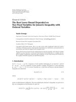
Figure 2 depicts the measurement layouts investigated. In
the first configuration (Figure 2(a)), a simple concrete wall of
thickness d
W
= 15.5ord
W
= 30 cm is present between two
ranging devices. In the second configuration (Figure 2(b)),
two walls of thicknesses 15 and 30 cm are present. Ranging
measurements were collected within 100cm of the walls to
minimize the influence of multipath and better capture the
DP excess delay effect. Specifically, ranging measurements
were collected for devices located 20, 40, 60, 80, and
100 cm from the surface of the walls. A total of 1500 range
measurements were collected for each configuration. Ta ble 1
reports the mean and standard deviation of the ranging error
in the collected measurements over all configurations for
each layout. As can be noted, the bias due to the excess delay
appears to increase linearly with the thickness of the wall.

The low value of the standard deviation indicates that the
4 EURASIP Journal on Advances in Signal Processing
d
W
Ranging device Ranging device
(a)
30 cm15 cm
Ranging device Ranging device
(b)
Figure 2: The configurations considered for DP excess delay
characterization. (a) 1 wall with thickness d
W
= 15.5cmord
W
=
30 cm; (b) 2 walls with combined thickness 15.5+30cm.
Table 1: Mean and standard deviation of ranging error for different
wall thicknesses.
Layout, d
W
[cm] Mean [cm] std dev [cm]
1 wall, 15.5 16.4 3.7
1 wall, 30 29.5 3.2
2walls,15.5 + 30 45.2 3
estimation error is dominated by the effects of DP excess
delay rather than multipath or distance-dependent received
power.
It is interesting to note that these numerical results can
also be considered as an indirect method to estimate the rel-
ative electrical permittivity


r
of the material under analysis
(in this case, concrete). The speed of the electromagnetic
wave travelling inside materials is slowed down by a factor
√

r
with respect to the speed of light, c  3·10
8
m/s; hence
the theoretical excess delay introduced by a wall of thickness
d
W
is
Δ
=

√

r
−1

d
W
c
. (1)
We observe in our measurements that Δ
 d
W

/c, and hence

r
 4, which is similar to the value obtained in [27].
3.2. Range estimation error
Section 3.1 shows that the excess delay is caused primarily
by the number and characteristics of the walls obstructing
the DP. We now use the data collected during the main
measurement campaign described in Section 2 to derive a
simple statistical model for ranging error. The collected
0
0.1
0.2
0.3
0.4
0.5
0.6
0.7
0.8
0.9
1
−50 −40 −30 −20 −100 1020304050
Ranging error (cm)
Measured data
Gaussian
CDF
Figure 3: CDF of the ranging error for the LoS condition.
Comparison with the Gaussian statistics.
ranging measurements were categorized and then analyzed
as a function of the number of walls between the ranging

devices. The ranging data was then analyzed as a function of
the number of walls between the ranging devices. Hence, the
data for each condition (LoS, NLoS 1 wall, NLoS 2 walls, etc.)
includes measurements taken at varying distances, positions
within the environment, wall thicknesses, and other factors.
Ta ble 2 reports the mean and standard deviation of the
ranging error for each condition, as well as the frequency
of the condition (number of configurations belonging to
the condition over the total number of configurations
considered). The characterization of the bias for 3,4, and 5
walls is not reported because the number of measurements
available was not sufficient to obtain a significant statistic.
As can be noted, the bias is strictly related to the number of
walls, regardless of the actual distance between the ranging
devices.
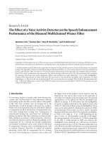
In Figures 3 and 4, the cumulative distribution functions
(CDF) for range measurements collected in the LoS, NLoS 1
wall, and NLoS 2 wall conditions are reported. These CDFs
are compared to the Gaussian CDF parameterized by the
mean and standard deviation values in Ta ble 2. In all cases,
there is a clear match between the measured data and the
Gaussian model.
3.3. Statistical model for ranging error
Let p
= (x, y)
T
be the vector of the target’s coordinates,
where the subscript T denotes the transpose. The true
distance to the ith beacon of known coordinates (x
i

, y
i
)is
given by
d
i
= d
i
(p) =


x −x
i

2
+

y − y
i

2
, i = 1, ,N. (2)
Davide Dardari et al. 5
Table 2: Mean, standard deviation, and frequency for ranging error in different wall conditions.
Condition Mean [cm] std dev [cm] Frequency
LoS 1.7 6.9 0.27
NLoS 1 wall 32.4 13.9 0.35
NLoS 2 walls 64.6 23.3 0.28
NLoS 3 walls N.A. N.A. 0.05
NLoS 4 walls N.A. N.A. 0.03

NLoS 5 walls N.A. N.A. 0.02
0
0.1
0.2
0.3
0.4
0.5
0.6
0.7
0.8
0.9
1
−100 −50 0 50 100 150 200
Ranging error (cm)
Measured data
Gaussian
1wall
2walls
CDF
Figure 4: CDF of the ranging error for the NLoS 1-wall and NLoS
2-wall conditions. Comparison with the Gaussian statistics.
We model the range measurement r
i
between the target and
the ith beacon as
r
i
= d
i
+ b

i
+ 
i
,(3)
where b
i
is the bias and 
i
is Gaussian noise, independent of
b
i
, with zero mean and variance σ
2
i
. The parameter σ
i
for the
scenario considered can be obtained from Ta ble 2 once the
number of walls between the ith beacon and the target node
is known.
The probability density function (p.d.f.) of

i
is therefore
given by
f

i
() =
1

√
2πσ
i
e
−
2
/2σ
2
i
. (4)
The bias b
i
can be treated either as a random variable, in case
a statistical characterization is available, or as a deterministic
quantity if it is somehow known. Below, we describe both
models of the bias.
3.3.1. Deterministic model for the bias
(wall extra delay model)
We have demonstrated that the bias depends primarily on the
walls obstructing the DP signal. The bias between the target
and the ith beacon, b
i
, can therefore be modelled as
b
i
= E
i
·c,
E
i

=
N
(i)
e

k=1
W
(i)
k
·Δ
k
,
(5)
where E
i
is the total time delay caused by NLoS conditions,
W
(i)
k
is the number of walls introducing the same excess delay
value Δ
k
(e.g., the number of walls of the same material and
thickness), and N
(i)
e
is the number of different excess delay
values. The total number of walls separating the ranging
devices is W
(i)

=

N
(i)
e
k=1
W
(i)
k
. We name this model the wall
extra delay (WED) model. When every wall in the scenario
has the same thickness and composition (i.e., Δ
k
= Δ for
each k), (5) simplifies to
b
i
= W
(i)
Δ·c. (6)
As will be demonstrated in Section 4, a priori knowledge
of the bias can sometimes be obtained using the WED model
if a preliminary estimate of the target position is available.
In that case, the approximate bias value can be simply
subtracted from the range measurements. The unbiased
distance estimates are then given by

d
i
= r

i
−b
i
(7)
with the following p.d.f., conditioned on the target position
p:
f
i
(

d
i
| p) ≡ f

i


d
i
−d
i

. (8)
3.3.2. Statistical model for the bias
Alternatively, the bias can be modeled using some priori
statistical characterization derived from measurements per-
formed in similar environments. From the results presented
earlier in the section, we can conclude that the bias will
always be nonnegative. A similar conclusion has been
attained by other authors, for example, [28]. The actual value

of the bias, however, will depend largely on the environment.
6 EURASIP Journal on Advances in Signal Processing
We expect the bias to take a wider range of values in
a cluttered environment with many walls, machines, and
furniture (such as a typical office building), than in an
open space. Note that the bias cannot grow infinitely large,
regardless of the propagation environment.
Although a detailed electromagnetic characterization of
the environment is rarely available, rough classification of
the environment is often feasible, for example, “concrete
office building” or “wooden warehouse.” By performing
range measurements in typical buildings of these classes
beforehand, we can assemble a library of histograms to
characterize ranging in various environment classes. We can
then use these histograms to approximate the probability
density function (p.d.f.) of the biases in the particular
building of interest.
Let us assume such histograms are available for each
beacon. They may differ from beacon to beacon, so we index
them by the beacon number i.Theith histogram has K
(i)
bars, where the kth bar covers the range β
(i)
k
−1
to β
(i)
k
and has
height p

(i)
k
. We can therefore associate the p.d.f. of b
i
, f
b
i
(b),
to the histogram according to
f
b
i
(b) 
K
(i)

k=1
w
(i)
k
u
{β
(i)
k
−1
,β
(i)
k
}
(b), (9)

where w
(i)
k
= p
(i)
k
/(β
(i)
k
− β
(i)
k
−1
), u
{a,a

}
(b) = 1ifa ≤ b ≤ a

,
0 otherwise, and β
(i)
0
= 0. We note that if the DP to beacon
i is LoS (i.e., the associated range measurement has no bias),
then f
b
i
(b) = δ(b), where δ(b) is the Dirac delta function.
In the absence of an appropriate histogram, the p.d.f.

of b
i
can be built using topological knowledge of the
environment and the WED model (5), with parameters taken
from measurements performed in a similar environment
class. In this case, K
(i)
= N
(i)
e
, β
(i)
k
= Δ
k
·c,andp
(i)
k
can be
taken as the frequency of all the configurations with the same
extra propagation delay Δ
k
between the ith beacon and the
target. For example, for the scenario considered, p
(i)
k
equals
the frequencies reported in the third column of Ta bl e 2.
Even in the absence of any measured data, we can
always determine the maximum expected bias β

m
for a fixed
scenario and, in the absence of other priori information,
assume a uniform distribution in [0, β
m
], that is, K = 1,
β
1
= β
m
,andw
1
= 1/β
m
[6].
To derive the complete statistical model for range
measurements, let us lump the bias term with the Gaussian
measurement noise
ν
i
= b
i
+
i
and obtain the corresponding
p.d.f.
f
ν
i



ν
i

=

∞
−∞
f
b
i
(x) f

i
(ν
i
−x)dx
=
K
(i)

k=1
w
(i)
k

Q


ν

i
−β
(i)
k
σ
i

−
Q


ν
i
−β
(i)
k
−1
σ
i

,
(10)
where Q(x)
= (1/
√
2π)

+∞
x
e

−t
2
/2
dt is the Gaussian Q-
function. If the ith beacon is LoS, then ν
i
is Gaussian
distributed with zero mean and variance σ
2
i
.Inorderto
obtain an unbiased estimator, we subtract the mean of
ν
i
,denotedm
i
, from the ith range measurement. This is
equivalent to replacing
ν
i
by ν
i
Δ
= ν
i
−m
i
.
The estimated distance is then modeled as


d
i
= d
i
+ ν
i
, (11)
with p.d.f. given by
f
i


d
i
| p

=
K
(i)

k=1
w
(i)
k

Q


d
i

−d
i
+ m
i
−β
(i)
k
σ
i

−
Q


d
i
−d
i
+ m
i
−β
(i)
k
−1
σ
i

.
(12)
Adifferent approach to modeling the ranging error

can be found in [21], where ranging data is analyzed as
a function of the true distance instead of the number of
walls. However, the Gaussian behavior of the ranging error
is also confirmed in that case. Expression (12) can be useful
to derive theoretical bounds on positioning; for example,
through the approach proposed in [6].
4. LOCALIZATION WITHOUT COOPERATION
The goal of positioning is to determine the locations of
the target(s), given a set of measurements (in our case
the ranges between nodes). Positioning occurs in two
steps. First, ranging measurements are obtained. Then, the
measurements are combined using positioning techniques
to deduce the location of the target(s). Depending on the
availability of a priori knowledge about the environment
topology and/or electromagnetic characteristics, different
positioning strategies can be adopted.
4.1. Localization without priori information
Multi-lateration is a practical method for determining a
node’s position. In the presence of ideal range measurements
(i.e.,

d
i
= d
i
), the ith beacon defines a circle centered in
(x
i
, y
i

)withradiusd
i
, upon which the target is located. If
the target has obtained ranges to multiple beacons, then
the intersection of the circles corresponds to the position of
the target node. In a two-dimensional space, at least three
beacons are required. Specifically, the position estimate (x, y)
is obtained by solving the following system of equations:

x
1
−x

2
+

y
1
− y

2
=

d
2
1
,
.
.
.


x
N
−x

2
+

y
N
− y

2
=

d
2
N
.
(13)
According to [25], the system of equations in (13)canbe
linearized by subtracting the last equation from the first N
−1
equations. The resulting system of linear equations is given
by the following matrix form:
A
·p = b, (14)
Davide Dardari et al. 7
where
A 

⎛
⎜
⎜
⎜
⎝
2(x
1
−x
N
)2(y
1
− y
N
)
.
.
.
.
.
.
2(x
N−1
−x
N
)2(y
N−1
− y
N
)
⎞

⎟
⎟
⎟
⎠
,
b 
⎛
⎜
⎜
⎜
⎝
x
2
1
−x
2
N
+ y
2
1
− y
2
N
+

d
2
N
−


d
2
1
.
.
.
x
2
N
−1
−x
2
N
+ y
2
N
−1
− y
2
N
+

d
2
N
−

d
2
N

−1
⎞
⎟
⎟
⎟
⎠
.
(15)
In a realistic scenario where ranging estimation errors are
present, (14) may be inconsistent, that is, the circles do
not intersect at one point. In that case, the position can be
estimated through a standard linear LS approach as
p =

A
T
A

−1
A
T
b, (16)
with the assumption that A
T
A is nonsingular and N ≥3[25].
Particular attention must be paid in selecting the beacon
associated with the last equation in (13) and used as reference
in (14), (15). If the corresponding range measurement is
biased, bias will be introduced in all the equations with
a consequent performance loss [29]. This aspect will be

investigated in the numerical results.
4.2. Localization with priori information
Our measurement results in Section 3 show that NLoS
configurations result in a ranging error bias which is often
the major source of positioning error. By analyzing this data,
we have also seen that the bias is strictly related to the number
of walls encountered by the signal. Assuming that priori
knowledge of the environment topology is available, it is
possible to refine the target’s position estimate once an initial
rough estimate has been obtained. In many cases, knowledge
of the room in which the target is located will suffice as an
initial estimate. These considerations suggest the following
two-step positioning algorithm when priori information is
available.
(i) First estimate: an initial rough position estimate
p
(1)
is
obtained using the LS method (16) by setting

d
i
= r
i
.
(ii) Range correction: biases due to propagation through
walls are subtracted from range measurements
according to (7) and the WED model for b
i
in (5),

where the number of walls separating the target and
each beacon is calculated using the first position
estimate and the topology information.
(iii) Refinement: a second LS position estimate
p
(2)
is cal-
culated with the corrected (unbiased) range values.
A possible improvement of this two-step algorithm is
to identify and select, based on the initial rough position
estimate, the reference beacon to be used in (13) during
the refinement step of LS position estimate. The reference
beacon can be chosen, for example, among those in LoS
condition or closer to the target node. In the numerical
results the impact of the reference beacon selection will be
investigated.
5. LOCALIZATION WITH COOPERATION
Let us now suppose that U
≥ 2 target nodes are present in the
same environment. In the absence of cooperation, each node
interacts only with the beacons and estimates its position
using, for example, the LS approach (16). It is expected that
if the targets are able to make range measurements not only
from the beacons but also from each other, thus cooperating,
then they can potentially improve their position estimation
accuracy.
We de fine M
= N + U as the total number of radio
devices (beacons plus targets) present in the system and r
i,m

for i,m = 1, 2, , M as the range measurements between the
ith and the mth devices. We do not consider ranges measured
between beacons. To make use of the range measurements
among target nodes, the following iterative LS algorithm is
proposed.
(1) Set n
= 1. Using (16) (or the two-step algorithm
described in Section 4.2), determine the position estimates
p
(1)
j
for the targets, that is, j = 1, 2, , U, by setting

d
i
=
r
i,j+N
with i = 1, 2, , N.
(2) Set n
= n +1.Foreachtarget j = 1, 2, , U, the
LS algorithm is applied by treating the other U
− 1targets
as additional “virtual” beacons located at the estimated
positions
p
(n)
j
obtained during the previous step. Specifically,
the matrices A

(n,j)
and b
(n,j)
at step n and for the jth target
are now
A
(n,j)

⎛
⎜
⎜
⎜
⎜
⎜
⎜
⎜
⎜
⎜
⎜
⎜
⎜
⎜
⎜
⎜
⎜
⎜
⎜
⎜
⎜
⎜

⎜
⎝
2

x
1
−x
N

2

y
1
− y
N

.
.
.
.
.
.
2

x
N−1
−x
N

2


y
N−1
− y
N

2

x
N+1
−x
N

2

y
N+1
− y
N

.
.
.
.
.
.
2

x
N+ j−1

−x
N

2

y
N+ j−1
− y
N

2

x
N+ j+1
−x
N

2

y
N+ j+1
− y
N

.
.
.
.
.
.

2

x
M
−x
N

2

y
M
− y
N

⎞
⎟
⎟
⎟
⎟
⎟
⎟
⎟
⎟
⎟
⎟
⎟
⎟
⎟
⎟
⎟

⎟
⎟
⎟
⎟
⎟
⎟
⎟
⎠
,
b
(n,j)

⎛
⎜
⎜
⎜
⎜
⎜
⎜
⎜
⎜
⎜
⎜
⎜
⎜
⎜
⎜
⎜
⎜
⎜

⎜
⎜
⎜
⎜
⎜
⎜
⎜
⎜
⎝
x
2
1
−x
2
N
+ y
2
1
− y
2
N
+

d
2
N
−

d
2

1
.
.
.
x
2
N
−1
−x
2
N
+ y
2
N
−1
− y
2
N
+

d
2
N
−

d
2
N
−1
x

2
N+1
−x
2
N
+ y
2
N+1
− y
2
N
+

d
2
N
−

d
2
N+1
.
.
.
x
2
N+ j
−1
−x
2

N
+ y
2
N+ j
−1
− y
2
N
+

d
2
N
−

d
2
N+ j
−1
x
2
N+ j+1
−x
2
N
+ y
2
N+ j+1
− y
2

N
+

d
2
N
−

d
2
N+ j+1
.
.
.
x
2
M
−x
2
N
+ y
2
M
− y
2
N
+

d
2

N
−

d
2
M
⎞
⎟
⎟
⎟
⎟
⎟
⎟
⎟
⎟
⎟
⎟
⎟
⎟
⎟
⎟
⎟
⎟
⎟
⎟
⎟
⎟
⎟
⎟
⎟

⎟
⎟
⎠
,
(17)
8 EURASIP Journal on Advances in Signal Processing
by setting

d
i
= r
i,j+N
for i = 1, 2, , M. The LS position
estimate for the jth target at step n is therefore
p
(n)
j
=

A
(n,j)
T
A
(n,j)

−1
A
(n,j)
T
b

(n,j)
. (18)
(3) If n
≥ N
iter
stop; else go to (2).
The algorithm stops when a predefined number N
iter
of
iterations is reached. Again, the reference beacon in (17)
can be selected when the reliability of range measurement is
known.
6. NUMERICAL RESULTS
In this section, we present a localization performance based
on experimental data. First, a scenario with only one target
(i.e., in the absence of cooperation) is considered.
Figure 5 shows the root mean square error (RMSE) of
the estimation for each location in the grid (identified by
the node ID) is reported for the case of N
= 3 (tx1,tx3,tx5)
and N
= 5 beacons. There is no priori information about
the environment topology, and beacon tx5 is chosen as the
reference node. It can be seen that for all locations the
use of a larger number of beacons does not necessarily
correspond to better positioning accuracy. This is due to
the fact that, in many cases, the added range measurements
and/or the chosen reference node are subject to large
errors, which cannot be corrected due to the absence of a
priori information. Moreover, the geometric configuration

of the additional beacons may not improve the positioning
accuracy in certain locations.
Next, we examine the effect of a priori information
and excess delay correction on positioning. The RMSE for
localization attained by the two-step algorithm presented
in Section 4.2 is reported in Figure 6. It can be seen that
positioning errors less than 1 meter are achieved in most
locations. By comparing Figures 5 and 6,wecanconclude
that the correction of the range measurements using the
WED model and knowledge of the environment topology
leads to a significant performance improvement for many
locations.
We mentioned in Section 4.2 that the wrong choice
of the reference beacon in the linear LS approach may
lead to significant performance degradation. This aspect is
investigated in Figure 7, where the best reference for each
target location is chosen from the set of 5 beacons, in order to
obtain the lowest RMSE with or without bias compensation.
By comparing Figure 7 with Figures 5 and 6,weobserve
that the selection of the right reference beacon can further
improve the positioning accuracy in both cases.
The effect of cooperation on localization is investigated
in Figures 8, 9,and10. Figure 8 presents the RMSE as a
function of the number of iterations N
iter
of the iterative
LS algorithm proposed in Section 5. We assume N
= 3
beacons (tx1,tx3,tx5) and two targets with the capability to
perform intertarget range measurements. Target 1 is located

in position 8, and the cooperating node (target 2) is located
in position 10 (LoS condition) or 18 (NLoS condition).
Beacon tx5 is assumed as reference for the LS algorithm.
These configurations were chosen because they lead to two
0
20
40
60
80
100
120
140
160
180
200
220
240
260
280
300
320
0 1 2 3 4 5 6 7 8 9 10 11 12 1314 15 16 17 18 19 20 21
Node ID
RMSE (cm)
5beacons
3beacons
Figure 5: RMSE as a function of target position in the absence of
priori information. N
= 3 (tx1,tx3,tx5) and N = 5 beacons are
considered.

0
20
40
60
80
100
120
140
160
180
200
220
240
260
280
300
320
0 1 2 3 4 5 6 7 8 9 10 11 12 1314 15 16 17 18 19 20 21
Node ID
RMSE (cm)
5beacons
3beacons
Figure 6: RMSE as a function of target position in the presence of
priori information (two-step algorithm). N
= 3 (tx1,tx3,tx5) and
N
= 5.
distinct interesting situations. When the two targets are
located in LoS, they can perform a highly accurate intertarget
range measurements. When the targets are located in NLoS

(different rooms), the intertarget range measurements are
expected to be worse. Figure 8 shows that cooperation in
LoS can strongly improve the RMSE and that the iterative
LS algorithm converges after few iterations. Note also that
the resulting RMSE for cooperation with 2 iterations and
N
= 3 beacons is better than the case of N = 5
beacons without cooperation (Figure 6). In Figure 9, the
same situation is considered, but the iterative LS algorithm
takes the cooperative node (target 2) as reference instead of
beacon tx5. Note that when the reference node is given by
a cooperative node in NLoS conditions with respect to the
Davide Dardari et al. 9
0
20
40
60
80
100
120
140
160
180
200
220
240
260
280
300
320

0 1 2 3 4 5 6 7 8 9 10 11 12 1314 15 16 17 18 19 20 21
Node ID
RMSE (cm)
Biased
Bias removed
Figure 7: RMSE as a function of target position in the absence
and presence of priori information (i.e., with the bias and after
removing the bias), using the best selection for reference beacon.
N
= 5 beacons are considered.
0
10
20
30
40
50
60
70
80
90
012345678
Number of iterations
RMSE (cm)
IDcoop = 10
IDcoop
= 18
Figure 8: RMSE as a function of number of iterations when target
1, located in position 8, cooperates with target 2, in position 10
or 18. N
= 3 (tx1,tx3,tx5) beacons are considered. Tx5 is taken as

reference for the LS algorithm.
target, for example, when target 2 is in position 10, the RMSE
increases with each iteration. Meanwhile, when target 2 is
in LoS, position 18, the RMSE remains roughly the same
after the second iteration. In Figures 9 and 10, we can also
compare the RMSE before the targets cooperate (iteration
1) to the RMSE after cooperation (iterations 2 and up). In
both cases, cooperation reduces the localization error when
the target nodes are in LoS.
Finally, in Figure 10 we examine localization perfor-
mance as a function of the position of the cooperating node.
0
20
40
60
80
100
120
140
160
180
200
220
240
260
280
300
320
012345678
Number of iterations

RMSE (cm)
IDcoop = 10
IDcoop
= 18
Figure 9: RMSE as a function of number of iterations when target
1, located in position 8, cooperates with target 2, in position 10 or
18. N
= 3 (tx1,tx3,tx5) beacons are considered. The cooperative
node is taken as reference for the LS algorithm.
0
10
20
30
40
50
60
70
80
90
Cooperative node ID
RMSE (cm)
0 1 2 3 4 5 6 7 8 9 10 11 12 13 14 15 16 17 18 19 20
Figure 10: RMSE as a function of target 2 position when target 1,
located in position 8, cooperates with target 2; N
= 3 (tx1,tx3,tx5)
beacons are considered, N
iter
= 4.
We consider the case of N = 3 beacons (tx1, tx3, tx5) and
N

iter
= 4 iterations when target 1, located in position 8,
cooperates with target 2, whose position varies. As can be
noted, the effect of cooperation varies with the position of
the cooperating node. In our scenario, the position of target 2
yielding the best performance is 10, in which the cooperating
node is in LoS. However, LoS positions 7 and 9 do not
lead to any performance gain. Moreover, positions 11 and
12 give significant improvement over the noncooperating
algorithm, despite the fact that the cooperating node is
in NLoS. Clearly, the intertarget link reliability and the
geometric configuration of the nodes both have significant
impacts in determining the localization error accuracy.
10 EURASIP Journal on Advances in Signal Processing
7. CONCLUSIONS
In this paper, the range estimation error between UWB
devices was characterized using measured data in a typical
indoor environment. These measurements showed that the
extra propagation delay is due primarily to the presence of
walls. A deterministic model (WED) for the extra propaga-
tion delay and a statistical model for the range estimation
error were proposed. A two-step LS positioning algorithm
incorporating the WED model was introduced to correct the
range measurements in NLoS conditions when the layout of
the environment is known. Results showed that a significant
gain in localization accuracy can be obtained by the two-
step algorithm and that an increase in the number of nodes
does not always result in performance gain, depending on the
geometric configuration of the nodes. In addition, the choice
of the reference node in the LS approach is an important

aspect that can have a significant impact on localization
accuracy.
An iterative LS algorithm was proposed to exploit
cooperation among targets. Results revealed that cooperation
is not always advantageous. In fact, it was shown that the
geometric configuration of the devices may have a stronger
impact than the quality of the intertarget range estimates on
the localization accuracy. This is an important consideration
when deriving guidelines for cooperation in positioning
algorithms.
ACKNOWLEDGMENTS
The authors would like to thank M. Chiani and H.
Wymeersch for helpful discussions. We also thank P. Pinto,
A. Giorgetti, N. Decarli, T. Pavani, R. Soloperto, L. Zuari,
and R. Conti for their cooperation during measurement
data collection and postprocessing. Finally, we would like
to thank O. Andrisano for motivating this work and for
hosting the measurement campaign at WiLAB. This work
has been performed in part within the framework of FP7
European Project EUWB (Grant no. 215669), the National
Science Foundation (Grant ECS-0636519) and Jet Propul-
sion Laboratory-Strategic University Research Partnership
Program.
REFERENCES
[1] R. J. Fontana and S. J. Gunderson, “Ultra-wideband precision
asset location system,” in Proceedings of the IEEE Conference
on Ultra Wideband Systems and Technologies (UWBST ’02),pp.
147–150, Baltimore, Md, USA, May 2002.
[2] L. Stoica, S. Tiuraniemi, A. Rabbachin, and I. Oppermann,
“An ultra wideband TAG circuit transceiver architecture,” in

Proceedings of the International Workshop on Ultra Wideband
Systems. Joint with Conference on Ultrawideband Systems and
Technologies (UWBST & IWUWBS ’04), pp. 258–262, Kyoto,
Japan, May 2004.
[3] D. Dardari, “Pseudo-random active UWB reflectors for accu-
rate ranging,” IEEE Communications Letters, vol. 8, no. 10, pp.
608–610, 2004.
[4] S. Gezici, Z. Tian, G. B. Giannakis, et al., “Localization via
ultra-wideband radios: a look at positioning aspects of future
sensor networks,” IEEE Signal Processing Magazine, vol. 22, no.
4, pp. 70–84, 2005.
[5] Y. Qi, H. Kobayashi, and H. Suda, “Analysis of wireless geolo-
cation in a non-line-of-sight environment,” IEEE Transactions
on Wireless Communications, vol. 5, no. 3, pp. 672–681, 2006.
[6] D. Jourdan, D. Dardari, and M. Z. Win, “Position error bound
for UWB localization in dense cluttered environments,” IEEE
Transactions on Aerospace and Electronic Systems, vol. 44, no.
2, pp. 613–628, 2008.
[7] M.Z.WinandR.A.Scholtz,“Ontherobustnessofultra-wide
bandwidth signals in dense multipath environments,” IEEE
Communications Letters, vol. 2, no. 2, pp. 51–53, 1998.
[8] M.Z.WinandR.A.Scholtz,“Ontheenergycaptureofultra
-wide bandwidth signals in dense multipath environments,”
IEEE Communications Letters, vol. 2, no. 9, pp. 245–247, 1998.
[9] M. Z. Win and R. A. Scholtz, “Characterization of ultra-
wide bandwidth wireless indoor channels: a communication-
theoretic view,” IEEE Journal on Selected Areas in Communica-
tions, vol. 20, no. 9, pp. 1613–1627, 2002.
[10] C C. Chong and S. K. Yong, “A generic statistical-based UWB
channel model for high-rise apartments,” IEEE Transactions on

Antennas and Propagation, vol. 53, no. 8, pp. 2389–2399, 2005.
[11] D. Cassioli, M. Z. Win, and A. F. Molisch, “The ultra-wide
bandwidth indoor channel: from statistical model to simula-
tions,” IEEE Journal on Selected Areas in Communications, vol.
20, no. 6, pp. 1247–1257, 2002.
[12] A. F. Molisch, D. Cassioli, C C. Chong, et al., “A compre-
hensive standardized model for ultrawideband propagation
channels,” IEEE Transactions on Antennas and Propagation,
vol. 54, no. 11, part 1, pp. 3151–3166, 2006.
[13] M. Z. Win and R. A. Scholtz, “Impulse radio: how it works,”
IEEE Communications Letters, vol. 2, no. 2, pp. 36–38, 1998.
[14] M. Z. Win and R. A. Scholtz, “Ultra-wide bandwidth time-
hopping spread-spectrum impulse radio for wireless multiple-
access communications,” IEEE Transactions on Communica-
tions, vol. 48, no. 4, pp. 679–689, 2000.
[15] W. Suwansantisuk and M. Z. Win, “Multipath aided rapid
acquisition: optimal search strategies,” IEEE Transactions on
Information Theory, vol. 53, no. 1, pp. 174–193, 2007.
[16] D. Dardari, C C. Chong, and M. Z. Win, “Improved lower
bounds on time-of-arrival estimation error in realistic UWB
channels,” in Proceedings of the IEEE International Conference
on Ultra-Wideband (ICUWB ’06), pp. 531–537, Waltham,
Mass, USA, September 2006.
[17] D. Dardari and M. Z. Win, “Threshold-based time-of-arrival
estimators in UWB dense multipath channels,” in Proceedings
of the IEEE International Conference on Communications (ICC
’06), vol. 10, pp. 4723–4728, Istanbul, Turkey, June 2006, Also
in IEEE Transactions on Communications, August 2008.
[18] C. Falsi, D. Dardari, L. Mucchi, and M. Z. Win, “Time of
arrival estimation for UWB localizers in realistic environ-

ments,” Eurasip Journal on Applied Signal Processing, vol. 2006,
Article ID 32082, p. 13, 2006.
[19] K. Yu and I. Oppermann, “Performance of UWB position
estimation based on time-of-arrival measurements,” in
Pro-
ceedings of the International Workshop on Ultra Wideband
Systems. Joint with Conference on Ultrawideband Systems and
Technologies (UWBST & IWUWBS ’04), pp. 400–404, Kyoto,
Japan, May 2004.
Davide Dardari et al. 11
[20] D. Dardari, A. Conti, U. Ferner, A. Giorgetti, and M. Z.
Win, “Ranging with ultrawide bandwidth signals in multipath
environments,” to appear in Proceedings of the IEEE,Special
Issue on UWB Technology & Emerging Applications, 2008.
[21] B. Alavi and K. Pahlavan, “Modeling of the TOA-based
distance measurement error using UWB indoor radio mea-
surements,” IEEE Communications Letters, vol. 10, no. 4, pp.
275–277, 2006.
[22] D. Jourdan, D. Dardari, and M. Z. Win, “Position error bound
for UWB localization in dense cluttered environments,” in
Proceedings of the IEEE International Conference on Communi-
cations (ICC ’06), vol. 8, pp. 3705–3710, Istanbul, Turkey, June
2006.
[23] E. G. Larsson, “Cram
´
er-Rao bound analysis of distributed
positioning in sensor netwroks,” IEEE Signal Processing Letters,
vol. 11, no. 3, pp. 334–337, 2004.
[24] N. Patwari, J. N. Ash, S. Kyperountas, A. O. Hero III, R. L.
Moses, and N. S. Correal, “Locating the nodes: cooperative

localization in wireless sensor networks,” IEEE Signal Process-
ing Magazine, vol. 22, no. 4, pp. 54–69, 2005.
[25] J. J. Caffery Jr., “A new approach to the geometry of TOA
location,” in Proceedings of the 52nd IEEE Vehicular Technology
Conference (VTC ’00), vol. 4, pp. 1943–1949, Boston, Mass,
USA, September 2000.
[26] D. Dardari and A. Conti, “A sub-optimal hierarchical max-
imum likelihood algorithm for collaborative localization in
ad-hoc network,” in Proceedings of the 1st Annual IEEE
Communications Society Conference on Sensor and Ad Hoc
Communications and Networks (SECON ’04), pp. 425–429,
Santa Clara, Calif, USA, October 2004.
[27] A. Muqaibel, A. Safaai-Jazi, A. Bayram, A. M. Attiya, and S.
M. Riad, “Ultrawideband through-the-wall propagation,” IEE
Proceedings—Microwaves, Antennas and Propagation, vol. 152,
no. 6, pp. 581–588, 2005.
[28] D. B. Jourdan, J. J. Deyst Jr., M. Z. Win, and N. Roy,
“Monte Carlo localization in dense multipath environments
using UWB ranging,” in Proceedings of the IEEE International
Conference on Ultra-Wideband (ICU ’05), pp. 314–319, Zurich,
Switzerland, September 2005.
[29] I. Guvenc, C C. Chong, and F. Watanabe, “Analysis of a
linear least-squares localization technique in LOS and NLOS
environments,” in Proceedings of the 65th IEEE Vehicular
Technology Conference (VTC ’07), pp. 1886–1890, Dublin,
Ireland, April 2007.