Báo cáo hóa học: "Research Article Rate-Optimized Power Allocation for DF-Relayed OFDM Transmission under Sum and Individual Power Constraints" pptx
Bạn đang xem bản rút gọn của tài liệu. Xem và tải ngay bản đầy đủ của tài liệu tại đây (872.5 KB, 11 trang )
Hindawi Publishing Corporation
EURASIP Journal on Wireless Communications and Networking
Volume 2009, Article ID 814278, 11 pages
doi:10.1155/2009/814278
Research Article
Rate-Optimized Power Allocation for DF-Relayed OFDM
Transmission under Sum and Individual Power Constraints
Luc Vandendorpe, J
´
er
ˆ
ome Louveaux, Onur Oguz, and Abdellat if Zaidi
Communications and Remote Sensing Laboratory, Universit
´
e Catholique de Louvain, Place du Levant 2,
1348 Louvain-la-Neuve, Belgium
Correspondence should be addressed to Luc Vandendorpe,
Received 10 November 2008; Revised 26 February 2009; Accepted 20 May 2009
Recommended by Erik G. Larsson
We consider an OFDM (orthogonal frequency division multiplexing) point-to-point transmission scheme which is enhanced by
means of a relay. Symbols sent by the source during a first time slot may be (but are not necessarily) retransmitted by the relay
during a second time slot. The relay is assumed to be of the DF (decode-and-forward) type. For each relayed carrier, the destination
implements maximum ratio combining. Two protocols are considered. Assuming perfect CSI (channel state information), the
paper investigates the power allocation problem so as to maximize the rate offered by the scheme for two types of power constraints.
Both cases of sum power constraint and individual power constraints at the source and at the relay are addressed. The theoretical
analysis is illustrated through numerical results for the two protocols and both types of constraints.
Copyright © 2009 Luc Vandendorpe et al. This is an open access article distributed under the Creative Commons Attribution
License, which permits unrestricted use, distribution, and reproduction in any medium, provided the original work is properly
cited.
1. Introduction
In applications where it is difficult to locate several antennas
on the same equipment, for size or cost issues, it has been
proposed to mimic multiantenna configurations by means
of cooperation among two or more terminals. Cooperation
or relaying, also coined distributed MIMO, has gained a lot
of interest recently. Cooperative diversity has been studied
for instance in [1–3] (and references therein) for cellular
networks.
In this paper we consider communication between a
source and a destination, and the source is possibly assisted
with a relay node. All the channels (source to destination,
source to relay and relay to destination) are assumed to
be frequency selective and in order to cope with that,
OFDM modulation with proper cyclic extension is used. The
relay operates in a DF mode. This mode is known to be
suboptimum [4, 5]. Decode-and-forward is adopted here as
a relaying strategy for its simplicity and its mathematical
tractability. Two protocols (P1 and P2) are considered. Each
protocol is made of two signaling periods, named time slots.
The first time slot is identical for both protocols. During this
period, on each carrier, the source broadcasts a symbol. This
symbol (affected by the proper channel gain) is received by
the destination and the relay. The relay may retransmit the
same carrier-specific symbol to the destination during the
second time slot. Whether the relay does it or not will be
indicated by the optimization problem which is formulated
and solved in this paper. The protocol P2 differs from the
protocol P1 in that, in the latter, the source does not transmit
during the second time slot, irrespective to whether the relay
is active or not during the second time slot. For P2, on a per
carrier basis, the source sends a new symbol if the relay is
inactive. The reason for not having the source and the relay
transmitting at the same time is to avoid the interference that
would occur in this case, thus rendering the optimization
problem somewhat tedious. Moreover in practice source
and relay will have different carrier frequency offsets which
is likely to require involved precorrection mechanisms. A
scenario with interference will be investigated in the future.
For both protocols, whenever it is active, the relay uses
the same carrier as the one used by the source. This is an
apriorichoicemadeheretomaketheoptimizationmore
tractable. It is however clear that carrier pairing between
source and relay is a topic for possible further optimization
of the scheme. At the destination, it is assumed that for
2 EURASIP Journal on Wireless Communications and Networking
the relayed carriers, the receiver performs maximum ratio
combining of what is received from the source in the first
time slot, and what is received from the relay in the second
one, for each tone.
OFDM with relaying has already been investigated by
some authors. In [6], the authors consider a general scenario
in which users communicate by means of OFDMA (orthog-
onal frequency division multiple access). They propose a
general framework to decide about the relaying strategy, and
the allocation of power and bandwidth for the different users.
The problem is solved by means of powerful optimization
tools, for individual constraints on the power. In the current
paper, we restrict ourselves to a single user scenario but
we investigate more deeply the analytical solution and its
understanding. We study power allocation to maximize the
rate for both cases of sum power and individual power
constraints. We also compare two different DF protocols and
show the advantage of having the source also transmitting
during the second time slot. In [7] the authors consider
a setup which is similar to the one we address in this
paper but with nonregenerative relays. In [8], the authors
investigate OFDM transmission with DF relaying, and a rate
maximizing power allocation for a global power constraint.
They briefly investigate the power allocation for the protocol
named P1 in the current paper, and a sum power constraint
only. On the other hand they investigate optimized tone
pairing. In [9], the authors consider OFDM with multiple
decode and forward relays. They minimize the total trans-
mission power by allocating bits and power to the individual
subchannels. A selective relaying strategy is chosen. More
recently, in [10] the authors also consider OFDM systems
assisted by a single cooperative relay. The orthogonal half-
duplex relay operates either in the selection detection-and-
forward (SDF) mode or in the amplify-and-forward (AF)
mode. The authors target the minimization of the transmit-
power for a desired throughput and link performance. They
investigate two distributed resource allocation strategies,
namely flexible power ratio (FLPR) and fixed power ratio
(FIPR).
The paper is organized as follows. The system under con-
sideration is described in Section 2. The rate optimization
for a sum power constraint is investigated in Section 3 for
the two protocols. The cases of individual power constraints
are dealt with in Section 4. Finally numerical results are
discussed in Section 5.
2. System Description
We consider communication between a source and a des-
tination, assisted with a relay node. All links are assumed
to be frequency selective and this motivates the use of
OFDM as a modulation technique. Assuming that the
cyclic prefix is properly designed and that transmission over
all links is synchronous, the scheme can be equivalently
represented by a set of parallel subsystems corresponding
to the different subchannels or frequencies used by the
modulation and facing flat fading over each link. The block
diagram associated with the system for one particular carrier
(or tone) is depicted in Figure 1.
Relay
Source
Destination
P
s
(k)
P
r
(k)
λ
sr
(k)
λ
rd
(k)
λ
sd
(k)
Figure 1: Structure of the system for carrier k.
During the first time slot, the source sends one modu-
lated symbol on each carrier. During the second time slot, the
relay selects some of the modulated symbols that it decodes,
and retransmits them. For each relayed symbol, we constrain
the relay to use the same carrier as that used by the source
for the same symbol. Based on the two signalling intervals,
the destination implements maximum ratio combining for
the carriers with relaying. As explained earlier, we consider
two protocols, called P1 and P2. In protocol P1, the carriers
that are not relayed are simply not used in the second time
slot (neither by the relay nor by the source). In protocol P2,
a new carrier specific modulated symbol is sent by the source
in the second time slot on each one of the carriers that are
not used by the relay.
Let us denote by A
s
(k)(resp.,A
r
(k)) the amplitude of
the symbol sent by the source (resp., the relay) on carrier
k in the first (resp., second) time slot, and by λ
sd
(k)(resp.,
λ
rd
(k)) the complex channel gain for tone k between source
(resp., relay) and destination. The noise sample corrupting
the transmission on tone k during the first time slot is n
s
(k),
and n
r
(k) during the second period. These two noise samples
are zero-mean circular Gaussian, white and uncorrelated
with the same variance σ
2
n
. Denoting by s(k) the unit variance
symbol transmitted over tone k, after proper maximum ratio
combining at the destination, the decision variable obtained
at the kth output of the FFT (Fast Fourier transform) is given
by
r
(
k
)
= A
2
s
(
k
)
|λ
sd
(k)|
2
s
(
k
)
+ A
2
r
(
k
)
|λ
rd
(k)|
2
s
(
k
)
+ A
s
(
k
)
λ
∗
sd
(
k
)
n
s
(
k
)
+ A
r
(
k
)
λ
∗
rd
(
k
)
n
r
(
k
)
.
(1)
The associated signal to noise ratio is given by
γ
(
k
)
=
P
s
(
k
)
|λ
sd
(
k
)
|
2
+ P
r
(
k
)
|λ
rd
(
k
)
|
2
σ
2
n
,(2)
where we have used the following notations: P
s
(k) = A
2
s
(k)
and P
r
(k) = A
2
r
(k).
3. Rate Optimization for
a Sum Power Constraint
We first investigate the case of a sum power constraint. The
techniques used in this section will be useful in solving
the problem with individual power constraints. It is well
known [11, 12] that the optimization with individual power
EURASIP Journal on Wireless Communications and Networking 3
constraints can be solved by reformulating it properly into
an equivalent problem with a sum power constraint. All
channels gains are assumed to be perfectly known for the
central device computing the power allocation. The overhead
associated with channel updating is not discussed further in
the current paper.
We investigate the two protocols separately.
3.1. Protocol P1. For protocol P1, the rate achieved by the
system for a duration of 2 OFDM symbols is given by [13]:
R
=
k∈S
s
log
1+
P
s
(
k
)
|λ
sd
(
k
)
|
2
σ
2
n
+
k∈S
r
min
log
1+
P
s
(
k
)
|λ
sr
(k)|
2
σ
2
n
,
log
1+
P
s
(
k
)
|λ
sd
(
k
)
|
2
+ P
r
(
k
)
|λ
rd
(k)|
2
σ
2
n
,
(3)
where S
s
is the set of carriers (or tones) receiving power at the
source only, and S
r
the complementary set, that is the set of
carriers receiving power at both source and relay. These sets
are not known in advance and must be characterized in an
optimal way. In [13] the signal to noise ratio without fading
was assumed to be symmetric throughout the network. Here
the model is more general and notations are introduced
to possibly allow different transmit powers at the source
and at the relay, not only for the same carrier but also for
different carriers. For a relayed carrier, assuming a decode-
and-forward mode, the rate is the minimum between the rate
on link s
→ d and the rate on the link s → r. The power
allocation which maximizes (3)isfirstinvestigatedforasum
power constraint
N
t
k=1
[
P
s
(
k
)
+ P
r
(
k
)
]
≤ P
t
,(4)
where P
t
is the total power budget available for the source
and the relay together, and N
t
is the total number of carriers.
Below, the objective function will be worked out in order to
find criteria enabling to decide about the set S
s
or S
r
to which
each carrier has to be assigned.
The Lagrangian for the optimization of the rate, taking
into account the total power constraint and the decode-and-
forward constraints, is defined by
L
1
=
k
i
k
log
1+
P
s
(
k
)
|λ
sd
(
k
)
|
2
σ
2
n
+
k
(
1
−i
k
)
log
1+
P
s
(
k
)
|λ
sd
(
k
)
|
2
+ P
r
(
k
)
|λ
rd
(
k
)
|
2
σ
2
n
−
μ
⎡
⎣
k
i
k
P
s
(
k
)
+
k
(
1
−i
k
)
[
P
s
(
k
)
+ P
r
(
k
)
]
−P
t
⎤
⎦
−
k
ρ
k
(
1
−i
k
)
P
s
(
k
)
|λ
sd
(
k
)
|
2
+ P
r
(
k
)
|λ
rd
(
k
)
|
2
−P
s
(
k
)
|λ
sr
(k)|
2
,
(5)
where μ is the Lagrange multiplier associated with the global
power constraint and ρ
k
is the Lagrange multiplier asso-
ciated with the decodability (perfect decode and forward)
constraint on carrier k.Thei
k
are indicators taking values
0 or 1 and whose optimization will provide the solution for
the assignment to sets S
s
(i
k
= 1) and S
r
(i
k
= 0).
Let us first investigate whether the decodability con-
straints are active or not for relayed carriers. For relayed
carrier q, i
q
= 0. If a constraint is inactive, its associated
Lagrange multiplier is zero [14]. Assuming this may be the
case, setting the ρ
q
= 0 and taking the derivative of the
Lagrangian with respect to the powers for a relayed carrier
leads to
∂R
∂P
s
q
=
1+
P
s
(q)
λ
sd
(q)
2
+ P
r
(q)
λ
rd
(q)
2
σ
2
n
−1
×
λ
sd
(q)
2
σ
2
n
= μ,
∂R
∂P
r
q
=
1+
P
s
(q)
λ
sd
(q)
2
+ P
r
(q)
λ
rd
(q)
2
σ
2
n
−1
×
λ
rd
(q)
2
σ
2
n
= μ.
(6)
This shows that assuming that the constraint is not saturated,
the equations lead to
|λ
sd
(q)|
2
=|λ
rd
(q)|
2
.Thisimposes
a constraint on the current channel state, which is almost
certain not to happen. Hence, except in very marginal cases,
the decode-and-forward constraint has to be saturated. This
means
P
s
(
k
)
|λ
sr
(k)|
2
= P
s
(
k
)
|λ
sd
(
k
)
|
2
+ P
r
(
k
)
|λ
rd
(
k
)
|
2
,
P
s
(
k
)
=
|
λ
rd
(k)|
2
P
r
(
k
)
|λ
sr
(k)|
2
−|λ
sd
(
k
)
|
2
= α
(
k
)
P
r
(
k
)
,
(7)
where the last line defines the coefficient α(k).
Hence for relayed carrier k, the total amount of power
P(k) allocated to that carrier will be given by P(k)
= P
s
(k)+
P
r
(k) = (1 + α(k)) P
r
(k) = P
s
(k)(1 + α(k))/α(k). Therefore
the Lagrangian can be written as:
L
2
=
k
i
k
log
1+
P
(
k
)
|λ
sd
(
k
)
|
2
σ
2
n
+
k
(
1
−i
k
)
log
1+
P
(
k
)
|λ
sr
(k)|
2
σ
2
n
α
(
k
)
1+α
(
k
)
−μ
⎡
⎣
k
i
k
P
(
k
)
+
k
(
1
−i
k
)
P
(
k
)
−P
t
⎤
⎦
,
(8)
where for k
∈ S
s
, P(k) = P
s
(k)andP
r
(k) = 0, while for
k
∈ S
r
, P(k) = P
s
(k)+P
r
(k)withP
s
(k) = α(k) P
r
(k).
4 EURASIP Journal on Wireless Communications and Networking
The solution for the carrier assignment can be found by
taking the derivatives with respect to the indicators. We have
that
∂R
∂i
q
= log
⎛
⎝
1+
P
q
λ
sd
(q)
2
/σ
2
n
1+
P
q
λ
sr
(q)
2
/σ
2
n
α
q
/
1+α
q
⎞
⎠
,
⎧
⎨
⎩
> 0, i
q
= 1,
< 0, i
q
= 0.
(9)
It appears that when
λ
sd
(q)
2
≤
α
q
1+α
q
λ
sr
(q)
2
(10)
the carrier should have i
q
= 0andbeallocatedtosetS
r
.By
opposition, when
λ
sd
(q)
2
≥
α
q
1+α
q
λ
sr
(q)
2
(11)
the carrier should be allocated to set S
s
.
Investigating (3) it should be clear that when one has
|λ
sr
(q)|
2
≤|λ
sd
(q)|
2
, because of the min, the rate obtained
by allocating the carrier to the set S
s
will always be higher
than the rate obained if the carrier were allocated to S
r
.It
is worth noting that, if
|λ
sr
(q)|
2
≥|λ
sd
(q)|
2
, the inequality
between (α(q)/(1+α(q)))
|λ
sr
(q)|
2
and |λ
sd
(q)|
2
is equivalent
to the inequality between
|λ
rd
(q)|
2
and |λ
sd
(q)|
2
.Asamatter
of fact, with the definition of α(q),
α
q
1+α
q
λ
sr
(q)
2
=
λ
sr
(q)
2
λ
rd
(q)
2
λ
sr
(q)
2
−
λ
sd
(q)
2
+
λ
rd
(q)
2
.
(12)
Then,
λ
sr
(q)
2
λ
rd
(q)
2
λ
sr
(q)
2
−
λ
sd
(q)
2
+
λ
rd
(q)
2
≥
λ
sd
(q)
2
,
λ
sr
(q)
2
λ
rd
(q)
2
−
λ
sr
(q)
2
λ
sd
(q)
2
≥
λ
rd
(q)
2
−
λ
sd
(q)
2
λ
sd
(q)
2
,
λ
sr
(q)
2
λ
rd
q
2
−
λ
sd
q
2
≥
λ
sd
q
2
λ
rd
q
2
−
λ
sd
q
2
.
(13)
The above shows that
λ
sd
(q)
2
≤
α
q
1+α
q
λ
sr
(q)
2
⇐⇒
λ
sd
(q)
2
≤
λ
rd
(q)
2
.
(14)
This means that when
|λ
sr
(q)|
2
≥|λ
sd
(q)|
2
, the allocation
to S
s
or to S
r
of the carrier may be based on either
comparisons in (14) because they are equivalent. And in
short, to be relayed, a carrier should fulfil the following
two conditions simultaneously:
|λ
sr
(q)|
2
≥|λ
sd
(q)|
2
and
|λ
rd
(q)|
2
≥|λ
sd
(q)|
2
.
Now that the assignment is known, the Karush-Kuhn-
Tucker (KKT) optimality conditions are such that, at the
optimum, for k
∈ S
s
,
∂R
∂P
(
k
)
=
P(k)+
σ
2
n
|λ
sd
(k)|
2
−1
= μ (15)
for the carriers to be served, and for carrier k such that
∂R
∂P
(
k
)
<μ (16)
the power should be set to P(k)
= 0. For carriers k ∈ S
r
and
to be served with power,
∂R
∂P
q
=
P(k)+
σ
2
n
|λ
sr
(k)|
2
1+α(k)
α(k)
−1
= μ (17)
while if
∂R
∂P
q
<μ (18)
we should set P(q)
= 0.
All these derivations basically also show that, after the
assignment step, our constrained optimization problem
can actually be solved thanks to the seminal waterfilling
algorithm, applied to a water container built either from
σ
2
n
/|λ
sd
(k)|
2
or from (σ
2
n
/|λ
sr
(k)|
2
)((1 + α(k))/α(k)). The
latter values actually show that the constraint related to the
DF operating mode of the relay leads to particular values to
be used for the container. More specifically, for the set S
r
,
these values are modified values with respect to the
|λ
sr
(k)|
2
.
3.2. Protocol P2. In this case, the rate achieved by the system
over a duration of 2 OFDM symbols is given by [13]:
R
= 2
k∈S
s
log
1+
P
s
(
k
)
2
|λ
sd
(k)|
2
σ
2
n
+
k∈S
r
min
log
1+
P
s
(
k
)
|λ
sr
(k)|
2
σ
2
n
,
log
1+
P
s
(
k
)
|λ
sd
(k)|
2
+ P
r
(
k
)
|λ
rd
(k)|
2
σ
2
n
,
(19)
where S
s
is the set of carriers (or tones) receiving power at
the source only, and S
r
is the complementary set, that is,
carriers receiving power at both the source and the relay. We
also denote by P
s
(k) the power allocated to a carrier at the
source. If this carrier is not relayed, each protocol instant uses
P
s
(k)/2.
Analysis of this objective function shows that the DF
constraint is also saturated on all carriers using the relay, like
EURASIP Journal on Wireless Communications and Networking 5
for protocol P1. Hence for a relayed carrier with an allocated
power P(q) the rate evolves as
R
r
q
=
log
1+
P
q
|
λ
sr
(k)|
2
σ
2
n
α
q
1+α
q
. (20)
For a nonrelayed carrier q, and a total allocated power P(q)
(over the two instants), the rate evolves as
R
s
q
=
log
⎡
⎣
1+
P(q)
λ
sd
(q)
2
2 σ
2
n
2
⎤
⎦
. (21)
When
|λ
sd
(q)|
2
> |λ
sr
(q)|
2
(α(q)/(1 + α(q))) we have that
R
s
(q) >R
r
(q) for any value of P(q). On the contrary, when
|λ
sd
(q)|
2
< |λ
sr
(q)|
2
(α(q)/(1 + α(q))) we have R
s
(q) <R
r
(q).
HoweverthisisonlyvalidforP(q)
≤ λ
t
where
λ
t
= 4σ
2
n
λ
sr
(q)
2
α
q
/
1+α
q
−
λ
sd
(q)
2
λ
sd
(q)
4
. (22)
If P(q)
≥ λ
t
, even when |λ
sd
(q)|
2
< |λ
sr
(q)|
2
(α(q)/(1+α(q))),
the power is better used by allocating the carrier to set S
s
.
Let us define the following Lagrangian, with a Lagrange
multiplier μ associated with the global power constraint, and
taking into account the saturation of the DF constraints:
L
3
= R −μ
⎡
⎣
k∈S
s
P
s
(
k
)
+
k∈S
r
P
(
k
)
−P
t
⎤
⎦
(23)
with
R
= 2
k∈S
s
log
1+
P
s
(
k
)
2
|λ
sd
(k)|
2
σ
2
n
+
k∈S
r
log
1+
P
(
k
)
|λ
sr
(k)|
2
σ
2
n
α
(
k
)
1+α
(
k
)
.
(24)
Equating to 0 the derivatives of this Lagrangian with respect
to the power, we get for k
∈ S
s
,
P
s
(
k
)
= 2
1
μ
−
σ
2
n
|λ
sd
(
k
)
|
2
+
, (25)
where [
·]
+
stands for max [0,.]. Similarly, for k ∈ S
r
,
P
(
k
)
=
1
μ
−
σ
2
n
|λ
sr
(k)|
2
1+α(k)
α(k)
+
. (26)
Again the derivations show that the constrained optimization
problem can be solved using the waterfilling algorithm,
applied to a water container built either from σ
2
n
/|λ
sd
(k)|
2
or
from (σ
2
n
/|λ
sr
(k)|
2
)((1 + α(k))/α(k)). It is also important to
note that for the nonrelayed carriers two identical values have
to be used for the water container, corresponding to the two
protocol instants. At the end of the waterfilling one checks
if any of the relayed carriers receives an amount of power
larger than the threshold given by (22). If this happens, the
relayed carrier fulfilling this condition and for which the rate
increase is the largest one is moved from the set S
r
to the
set S
s
. The waterfilling is applied again. This procedure is
iterated till none of the relayed carrier receives an amount
of power larger than its associated threshold. In the sequel
this procedure will be named the reallocation step.
4. Rate Maximization for
Individual Power Constraints
This section is devoted to the power allocation which
maximizes the rates under individual power constraints on
the source and the relay respectively:
N
t
k=1
P
s
(
k
)
≤ P
s
, (27)
N
t
k=1
P
r
(
k
)
≤ P
r
. (28)
First, note that for the optimum power allocation with
individual power constraints, it might happen that constraint
(28) is inactive for certain values of channel parameters, but
constraint (4) will always be active. In other words, at the
optimum, the full available power will always be used at the
source, while some of the power available at the relay may
not be used. This can be explained using simple intuitive
arguments. Assume a solution is found such that P
s
is not
fully used. The rate can be further increased by allocating
the remaining source power to a carrier in set S
s
or in set
S
r
. For the relay power, things may be different. For instance,
it may even happen that all carriers are allocated to the set
S
s
in which case the relay does not transmit at all. One way
to take this particular case into account is to perform a first
optimization (called first step hereafter), trying to allocate
the source power in an optimum way, not considering the
constraint on the relay power. After this allocation process
of the source power, one has to check whether the relay
power is sufficientornot.Ifitissufficient, then the optimum
solution corresponds to this particular situation in which
the full relay power is not used. If not, it can now be
assumed that the relay power constraint is satisfied with
equality at the optimum, and the full iterative method
explained below should be used. Let us first describe the first
step.
4.1. First Step. Again, we analyze the two protocols sepa-
rately.
4.1.1. Protocol P1. Theprobleminthiscaseisstillto
maximize (3) where it is now assumed that the constraint on
P
r
may not be active. This means that there is enough relay
power such that for a relayed carrier k, P
r
(k) can always be
made large enough to have
P
s
(
k
)
|λ
sd
(k)|
2
+ P
r
(
k
)
|λ
rd
(k)|
2
≥ P
s
(
k
)
|λ
sr
(k)|
2
. (29)
As discussed above, the constraint on the source power
being saturated the associated Lagrange multiplier μ
s
may
be different from 0. Here we investigate a solution for the
case where the relay power is not saturated and the related
6 EURASIP Journal on Wireless Communications and Networking
Lagrange multiplier is then 0. The corresponding Lagrange
function can be written as:
L
4
=
k∈S
s
log
1+
P
s
(
k
)
|λ
sd
(k)|
2
σ
2
n
+
k∈S
r
log
1+
P
s
(
k
)
|λ
sr
(k)|
2
σ
2
n
−
μ
s
⎡
⎣
k∈S
s
P
s
(
k
)
−P
s
⎤
⎦
.
(30)
In agreement with the indicator variables used above, when
|λ
sd
(q)|
2
≥|λ
sr
(q)|
2
carrier q should be allocated to set S
s
.
In the reverse case, it should be allocated to set S
r
. Once the
assignment is known, taking the derivative with respect to
P
s
(q)withq ∈ S
s
and equating it to 0, it comes
∂R
∂P
s
q
=
D
q
(
P
s
)
=
P
s
(q)+
σ
2
n
λ
sd
(q)
2
−1
= μ
s
. (31)
For a carrier q in the other set, S
r
,weget
∂R
∂P
s
q
=
D
q
(
P
s
)
=
P
s
(q)+
σ
2
n
λ
sr
(q)
2
−1
= μ
s
. (32)
Hence the problem can be solved by means of a water-
filling procedure, where the container is built from values
σ
2
n
/|λ
sd
(q)|
2
in set S
s
,andvaluesσ
2
n
/|λ
sr
(q)|
2
in set S
r
.With
such an allocation procedure, the minimum power required
at the relay is given by
S
r
P
r
(q)whereP
r
(q) = P
s
(q)/α(q).
If this value is below the power available at the relay, the
problem is solved. This would correspond to a situation
where the relay is located far away from the source, and,
in a sense, not very useful for the protocol used here.
Otherwise one has to investigate the situation where both
power constraints are active (saturated), which is of most
interest.
4.1.2. Protocol P2. The corresponding Lagrange function can
be written:
L
5
= 2
k∈S
s
log
1+
P
s
(
k
)
2
|λ
sd
(k)|
2
σ
2
n
+
k∈S
r
log
1+
P
s
(
k
)
|λ
sr
(k)|
2
σ
2
n
−
μ
s
⎡
⎣
k∈S
s
P
s
(
k
)
−P
s
⎤
⎦
.
(33)
Taking the derivative with respect to P
s
(q)withq ∈ S
s
and
equating it to 0, it comes
∂R
∂P
s
q
= D
q
(
P
s
)
=
P
s
(q)
2
+
σ
2
n
λ
sd
(q)
2
−1
= μ
s
. (34)
For a carrier q in the other set, S
r
,
∂R
∂P
s
q
=
D
q
(
P
s
)
=
P
s
(q)+
σ
2
n
λ
sr
(q)
2
−1
= μ
s
. (35)
So the conclusions are similar to those drawn for protocol P1.
The problem can again be solved by means of a waterfilling
procedure, where the container is built from the values
σ
2
n
/|λ
sd
(q)|
2
, and the values σ
2
n
/|λ
sr
(q)|
2
in set S
r
.Howeverit
has to be noted that for the values related to set S
s
those values
have to be used twice because of the two time slots. Besides
that, the reallocation procedure has to be implemented: it has
to be checked whether any of the carrier allocated to set S
r
receives an amount of power above a certain threshold. If this
happens, carriers have to be moved from set S
r
to set S
s
,and
the waterfilling has to be applied till this no longer happens,
as explained above. The value to be used for the threshold
is similar to (22), where
|λ
sr
(q)|
2
has to be used instead of
|λ
sr
(q)|
2
α(q)/(1 + α(q)).
4.2. Second Step. A second step is needed unless the power
used at the relay by the procedure described in the first step
is below the available relay power. Two Lagrange multipliers,
μ
s
ad μ
r
, now have to be used for the power contraints.
One element in the direction of the solution lies in the
observation [12] that the rate only depends on the products
of powers and (possibly modified) channel gains. Hence
allocating power P to a carrier with gain
|λ|
2
provides the
same rate as allocating power μP to a carrier with gain
|λ|
2
/μ.
Let us assume for the moment that the optimum μ
s
and μ
r
are known. The allocation rules proposed above to define
the sets S
s
and S
r
should be revisited with gains modified as:
|λ
μ
sd
|
2
=|λ
sd
|
2
/μ
s
; |λ
μ
sr
|
2
=|λ
sr
|
2
/μ
s
and |λ
μ
rd
|
2
=|λ
rd
|
2
/μ
r
.
The equivalent powers under consideration are now P
μ
s
(q) =
μ
s
P
s
(q)andP
μ
r
(q) = μ
r
P
r
(q).
4.2.1. Protocol P1. Let us define the following Lagrangian:
L
μ
1
=
k
i
k
log
⎛
⎜
⎝
1+
P
μ
s
(
k
)
λ
μ
sd
(k)
2
σ
2
n
⎞
⎟
⎠
+
k
(
1
−i
k
)
log
⎛
⎜
⎝
1+
P
μ
s
(
k
)
λ
μ
sd
(
k
)
2
+P
μ
r
(
k
)
λ
μ
rd
(k)
2
σ
2
n
⎞
⎟
⎠
−
⎡
⎣
k
P
μ
s
(
k
)
−μ
s
P
s
⎤
⎦
−
⎡
⎣
k
(
1
−i
k
)
P
μ
r
(
k
)
−μ
r
P
r
⎤
⎦
−
k∈S
r
ρ
k
(
1
−i
k
)
P
μ
s
(
k
)
λ
μ
sd
(
k
)
2
+ P
μ
r
(
k
)
λ
μ
rd
(
k
)
2
−P
μ
s
(
k
)
λ
μ
sr
(
k
)
2
.
(36)
It is interesting to compare this Lagrangian with the one
given by (5). Actually they both have the same structure. The
EURASIP Journal on Wireless Communications and Networking 7
first difference is that (5)isbasedonP’s and λ’s while (36)is
based on P
μ
’s and λ
μ
’s. Assuming that μ
s
and μ
r
are known,
and thanks to the use of the modified gains and powers, the
individual power constraints give rise to a single sum power
constraint. The associated Lagrange multiplier now has to be
equal to 1.
Based on these observations, it turns out that for fixed
μ
s
and μ
r
all the results derived in Section 3 apply to
our problem with individual power constraints, and to the
powers and the gains that have been properly normalized. In
particular it can be concluded that for the carriers using the
relay, the decode-and-forward constraint will be saturated,
leading to P
μ
r
(q) = P
μ
s
(q)/α
μ
(q). Hence P
μ
r
(q)andP
μ
s
(q)
should be allocated simultaneously leading to a total power
denoted by P
μ
(q) = P
μ
r
(q)+P
μ
s
(q) = (1 + α
μ
(q))P
μ
r
(q) =
P
μ
s
(q)(1 + α
μ
(q))/α
μ
(q)where
α
μ
q
=
λ
μ
rd
(q)
2
λ
μ
sr
(q)
2
−
λ
μ
sd
(q)
2
=
μ
s
μ
r
α
q
. (37)
Considering that P
μ
(q) = P
μ
s
(q)(1 + α
μ
(q))/α
μ
(q), we also
have
P
μ
s
q
λ
μ
sr
(q)
2
= P
μ
q
λ
μ
sr
(q)
2
α
μ
q
1+α
μ
q
=
P
μ
(
k
)
λ
μ
sr
(k)
2
μ
s
α
(
k
)
μ
r
+ α
(
k
)
μ
s
= P
μ
q
λ
μ
sr
(q)
2
α
q
μ
r
+ μ
s
α
q
.
(38)
Therefore, omitting the indicators, the Lagrangian can be
rewritten as
L
μ
2
=
k∈S
s
log
⎛
⎜
⎝
1+
P
μ
s
(
k
)
λ
μ
sd
(k)
2
σ
2
n
⎞
⎟
⎠
+
k∈S
r
log
⎛
⎜
⎝
1+P
μ
(
k
)
λ
μ
sr
(k)
2
σ
2
n
μ
s
α
(
k
)
μ
r
+ α
(
k
)
μ
s
⎞
⎟
⎠
−
⎡
⎣
k
P
μ
s
(
k
)
+
k
P
μ
(
k
)
−μ
s
P
s
−μ
r
P
r
⎤
⎦
.
(39)
Carrier q should be placed in set S
s
if
λ
μ
sd
(q)
2
≥
λ
μ
sr
(q)
2
α
μ
q
1+α
μ
q
=
λ
sr
(q)
2
α
q
μ
r
+ α
q
μ
s
.
(40)
Based on the above, and relations (14)tobeadaptedwithλ
μ
and α
μ
it turns out that the selection rule when |λ
μ
sd
(q)|
2
≤
|
λ
μ
sr
(q)|
2
amounts to choosing S
s
when |λ
μ
sd
(q)|
2
≥|λ
μ
rd
(q)|
2
or when
λ
sd
(q)
2
λ
rd
(q)
2
≥
μ
s
μ
r
(41)
and vice-versa. Therefore, the allocation procedure of the
carriers turns out to be equivalent to that in the sum power
case, with properly modified channel gains.
There is however one important exception to this rule
which is related to the particular case where the equality
|λ
sd
(q)|=|λ
rd
(q)| holds. It has been assumed previously
that this particular case needs not being investigated as
it is very unlikely to happen. This applies for the sum
power constraint. However, in the case of individual power
constraints, the procedure is now working with the modified
values λ
μ
(q) which are no longer given but depend on the
Lagrange parameters μ
s
and μ
r
. It may happen (and has been
encountered for some of the channels randomly generated)
that the optimal values of these Lagrange parameters are such
that the equality is exactly met on some carriers (usually at
most one). This particular situation needs a few additional
developments and adjustments which have been presented
in [15] and will not be repeated here.
For a carrier belonging to the set S
s
, the rate gain and
optimality conditions are given by
∂R
∂P
μ
s
q
=
⎡
⎢
⎣
P
μ
s
(q)+
σ
2
n
λ
μ
sd
(q)
2
⎤
⎥
⎦
−1
= 1. (42)
This leads to
P
μ
s
q
=
1 −
σ
2
n
μ
s
λ
sd
(q)
2
+
. (43)
For a carrier belonging to the set S
r
, the gain and optimality
conditions are given by
∂R
∂P
μ
q
=
P
μ
(q)+
σ
2
n
λ
sr
(q)
2
μ
s
α(q)+μ
r
α(q)
−1
= 1.
(44)
The corresponding power allocation is given by
P
μ
q
=
1 −
σ
2
n
λ
sr
(q)
2
μ
r
+ α(q)μ
s
α(q)
+
. (45)
So far, we have assumed that μ
r
and μ
s
were known.
In fact there is a single pair (μ
s
, μ
r
) for which the two
power constraints are simultaneously fulfilled. To find this
pair, the following algorithm is proposed. The idea is to
scan all possible assignments to sets S
s
and S
r
. For carriers
such that
|λ
sd
(q)|
2
≥|λ
sr
(q)|
2
, as discussed above, the
carrier will be assigned to set S
s
. For the other carriers, with
|λ
sd
(q)|
2
≤|λ
sr
(q)|
2
, relaying may be considered. Equation
(41) says that the assignment of a carrier candidate for
relaying depends on the ratio
|λ
rd
(q)|
2
/|λ
sd
(q)|
2
. By sorting
the carriers candidates for relaying by decreasing order of
the ratios
|λ
rd
(q)|
2
/|λ
sd
(q)|
2
, all possible assignments can
be considered. As a matter of fact, if a single carrier gets
relayed it will be the first one in the sorted set. If two get
relayed, it will be the first two, and so forth. Therefore, by
considering all possible sets of first carriers in this sorted set,
all possible assignments can be investigated. We have as many
8 EURASIP Journal on Wireless Communications and Networking
situations to consider as we have carriers being candidates to
be relayed. For each situation, the assignment to sets S
s
and
S
r
is fixed. For a fixed assignment, the optimization problem
to be solved is convex. The corresponding dual problem is
also convex. The dual problem can be solved by taking the
derivativesofthedualobjectivewithrespecttoμ
s
and μ
r
,
and equating these derivatives to zero. The values of μ
∗
s
and
μ
∗
r
solving these equations can be entered in the primal
problem, and the optimum power values can be obtained.
The problem is that the equations to find the optimum μ
s
and μ
r
are nonlinear. They can be solved for instance in an
iterative manner.
These derivatives with respect to μ
s
and μ
r
correspond
to the two power constraints that have to be fulfilled. Hence
any classical method known to find the roots of a function
(herethederivativeswithrespecttoμ
s
and μ
r
)canbeused.
A typical method used is the so-called “subgradient method”
where the correction to the Lagrange variables μ
s
and μ
r
at
step i is made proportionally to the error on the constraints.
Here we try to improve this classical method by using a
Newton-Raphson algorithm where the first derivative of the
objective function (here the objectives are the constraints)
is also used. A Newton-Raphson approach is known to have
quadratic convergence, and to always converge for a convex
objective function. At iteration i, the power prices μ
r
and μ
s
are updated according to
⎡
⎣
μ
i+1
s
μ
i+1
r
⎤
⎦
=
⎡
⎣
μ
i
s
μ
i
r
⎤
⎦
−
λ
⎡
⎢
⎢
⎢
⎣
∂
q
P
s
(q)
∂μ
s
∂
q
P
s
(q)
∂μ
r
∂
q
P
r
(q)
∂μ
s
∂
q
P
r
(q)
∂μ
r
⎤
⎥
⎥
⎥
⎦
−1
×
⎡
⎢
⎣
q
P
s
q
−
P
s
q
P
r
q
−
P
r
⎤
⎥
⎦
.
(46)
This Newton-Raphson procedure is thus to be repeated for
each one of the possible assignments.
4.2.2. Protocol P2. Adapting the results of the previous
subsection leads to the following Lagrangian with the
modified gains and powers:
L
μ
3
= 2
k∈S
s
log
⎛
⎜
⎝
1+
P
μ
s
(
k
)
2
λ
μ
sd
(k)
2
σ
2
n
⎞
⎟
⎠
+
k∈S
r
log
⎛
⎜
⎝
1+P
μ
(
k
)
λ
μ
sr
(k)
2
σ
2
n
μ
s
α
(
k
)
μ
r
+ α
(
k
)
μ
s
⎞
⎟
⎠
−
⎡
⎣
k
P
μ
s
(
k
)
+
k
P
μ
(
k
)
−μ
s
P
s
−μ
r
P
r
⎤
⎦
.
(47)
For a carrier belonging to the set S
s
, the rate gain and
optimality conditions are given by
∂R
∂P
μ
s
q
=
⎡
⎢
⎣
P
μ
s
(q)
2
+
σ
2
n
λ
μ
sd
(q)
2
⎤
⎥
⎦
−1
= 1 (48)
which leads to
P
μ
s
q
=
2
1 −
σ
2
n
μ
s
λ
sd
(q)
2
+
. (49)
For a carrier belonging to the set S
r
, the gain and optimality
conditions are given by
∂R
∂P
μ
q
=
P
μ
(q)+
σ
2
n
λ
sr
(q)
2
μ
s
α(q)+μ
r
α(q)
−1
= 1.
(50)
The corresponding power allocation is given by
P
μ
q
=
1 −
σ
2
n
λ
sr
(q)
2
μ
r
+ α(q)μ
s
α(q)
+
. (51)
Equations (49)and(51) also show that the powers are given
by a waterfilling procedure with a common water level 1
or a common power constraint, and containers defined by
these equations. The problem is again equivalent to the sum
power case and the procedure defined for the maximisation
problem in Section 3.2 can be reused. The
|λ
sd
(q)|
2
have to
be replaced by
|λ
sd
(q)|
2
/μ
s
, and the |λ
sr
(q)|
2
α(q)/(1 + α(q))
by
|λ
sr
(q)|
2
α(q)/(μ
r
+ α(q)μ
s
). The comments about the
allocation of the carrier to set S
s
or S
r
are the same as in the
case of protocol P1. Recall also that the reallocation step has
to be implemented. The Newton-Raphson procedure for the
updating of μ
s
and μ
r
is similar to that used for protocol P1.
5. Results
In order to illustrate the theoretical analysis, numerical
results are provided and discussed. The number of carriers
is set to N
t
= 128. Channel impulse responses (CIR) of
length 32 are generated. The taps are randomly generated
from independent zero mean unit variance circular complex
gaussian distributions. Hence the power delay profile is flat.
All taps have a unit variance for all links. From these CIRs,
FFT are computed to provide the corresponding λ
xy
(x ∈
{
s, r}, y ∈{r, d}). We set σ
2
n
= 1.
For illustrative purposes, results are first presented for
one particular channel realization. The power is set to
P
t
= 200 for the sum power constraint, and to P
s
=
100 and P
r
= 100 for the case of individual power
constraints. Figure 2 shows the gains
|λ
sr
(k)|
2
(solid curve),
|λ
sd
(k)|
2
(dash-dotted), |λ
rd
(k)|
2
(dashed) in dBW of the
channels. Figure 3 shows, for protocol P1 and the sum power
constraint, the result about the power allocation (
◦)and
the possible additional split whenever relevant among source
power (solid line) and relay power (dashed). The
×s indicate
whether the relay is active (
× at the top of the figure) or not
(
× in 0). In this case, the power used by the source is 136
and that by the relay is 64. The total rate obtained here is
275.45 bits per a duration of 2 OFDM symbols. If preferred,
this rate N
b
(bits) per 2 OFDM symbols may readily be
converted to a spectral efficiency by computing N
b
/2N
t
(1+β)
(bits/sec/Hz) where β is the roll-off factor. Figure 4 reports
the power allocation for protocol P2 with a sum power
EURASIP Journal on Wireless Communications and Networking 9
−20
−15
−10
−5
0
5
10
15
(dB)
0 20 40 60 80 100 120 140
Carrier position
Frequency responses of the different channels (dB)
LSR
LSD
LRd
Figure 2: Gains |λ
sr
(k)|
2
, |λ
sd
(k)|
2
, |λ
rd
(k)|
2
in dBW.
0
0.5
1
1.5
2
2.5
0 20 40 60 80 100 120 140
Carrier position
Power allocated to source and to relay
To t a l p o w e r
Source power
Relay power
Relay indic
Figure 3: Final power allocation to source and relay in the sum
power case and protocol P1.
constraint. Recall that for a nonrelayed carrier the amount
of source power shown has to be used twice: once per time
slot. The rate achieved for the particular channel realization
under consideration here is 377.45 bits for a duration of 2
OFDM symbols. It is also interesting to mention that in
this case, the power allocated to the source for the channel
realization under consideration is 186.8 and to the relay, the
remainder meaning 13.2. Compared to protocol P1, the gain
is noticeable and is clearly due to the better exploitation of
the second time slot.
0
0.5
1
1.5
2
2.5
3
3.5
0 20 40 60 80 100 120 140
Carrier position
Power allocated to source and to relay
To t a l p o w e r
Source power
Relay power
Relay indic
Figure 4: Final power allocation to source and relay in the sum
power case for protocol P2.
0
200
400
600
800
1000
1200
1400
1600
Rate (bits)
0 5 10 15 20 25 30
P
t
(dBW)
P1+P2: rate versus power sum optimum /uniform
LSR 100 LSD LRD 1
P1opt
P2opt
P1 unif
P2 unif
Figure 5: Rate versus P
t
(dBW) for the two protocols and uniform
and optimized power allocation for the sum power constraint. Taps
of the
|λ
sr
(k)|
2
have a variance 20 dBs above those associated with
the
|λ
sd
(k)|
2
and the |λ
rd
(k)|.
With protocol P1 and individual power constraints, the
bit rate achieved is 239.74 bits for a duration of 2 OFDM
symbols. Compared to the same protocol with the sum
power constraint, the observed rate loss is due to the values
chosen here for the individual power constraints (100-100)
which are rather different from the values devoted to the
two categories of carriers by the sum power case (136-64).
For individual power constraints and protocol P2, the total
rate is 318 bits per 2 OFDM symbols duration. The loss
incurred compared to the sum power case can be explained
10 EURASIP Journal on Wireless Communications and Networking
−5
0
5
10
15
20
25
30
35
Rate gain (%)
0 5 10 15 20 25 30
P
t
(dBW)
P1+P2: rate versus power sum optimum /uniform
LSR 100 LSD LRD 1
P1
P2
Figure 6: Rate gain with the optimized power allocation compared
to the uniform one, versus P
t
(dBW) for the two protocols and the
sum power constraint. Taps of the
|λ
sr
(k)|
2
have a variance 20 dBs
above those associated with the
|λ
sd
(k)|
2
and the |λ
rd
(k)|
2
.
in a manner identical to that discussed for protocol P1. And
again the advantage of this protocol compared to P1 is visible.
Systematic results have also been produced for the two
protocols, the sum power case, and different values of P
t
.
For each value of P
t
the results reported are obtained by
averaging over 250 channel realizations. The CIRs associated
with the
|λ
sr
(k)|
2
, have a variance of 20 dBs above those
associated with the
|λ
sd
(k)|
2
and the |λ
rd
(k)|
2
. The results
obtained with the optimized power allocation are contrasted
against uniform power allocation. For protocol P1 with
uniform power allocation, the carrier allocation to sets S
s
and
S
r
is performed as in the optimized case. The power available
is uniformly divided between the N
t
carriers. For the carriers
to be relayed, the per carrier power is further split between
source and relay according to the ratio associated with the
saturation of the decodability constraint (7). For protocol P2,
the allocation of the carrier to set S
s
or S
r
is based on the
comparison of
|λ
sd
(q)|
2
with |λ
sr
(q)|
2
(α(q)/(1+α(q))). If N
s
carriers are allocated to set S
s
and N
t
− N
s
to set S
r
the total
power is divided by 2N
s
+ N
t
− N
s
= N
t
+ N
s
in order to
take into account the use of the two time slots for the carriers
in S
s
. At this point the reallocation step is implemented and
some carriers may be moved from S
r
to S
s
. For the carriers
remaining in set S
r
the power is further split among source
and relay according to the ratio associated with the saturation
of the decodability constraint (7). Figure 5 reports the rate
obtained with the two protocols, and for each protocol, with
the optimized and the uniform power allocation. In order
to have a better understanding of the gain associated with
the optimized power allocation with respect to the uniform
one, the rate gain in % between uniform power allocation
0
200
400
600
800
1000
1200
1400
1600
Rate (bits)
0 5 10 15 20 25 30
P
t
(dBW)
P1+P2: rate versus power sum optimum /uniform
LSR 10 LSD LRD 1
P1opt
P2opt
P1 unif
P2 unif
Figure 7: Rate versus P
t
(dBW) for the two protocols and uniform
and optimized power allocation for the sum power constraint. Taps
of the
|λ
sr
(k)|
2
have a variance 10 dBs above those associated with
the
|λ
sd
(k)|
2
and the |λ
rd
(k)|
2
.
−5
0
5
10
15
20
25
30
35
40
Rate gain (%)
0 5 10 15 20 25 30
P
t
(dBW)
P1+P2: rate versus power sum optimum /uniform
LSR 10 LSD LRD 1
P1
P2
Figure 8: Rate gain with the optimized power allocation compared
to the uniform one, versus P
t
(dBW) for the two protocols and the
sum power constraint. Taps of the
|λ
sr
(k)|
2
have a variance 10 dBs
above those associated with the
|λ
sd
(k)|
2
and the |λ
rd
(k)|
2
.
and optimized allocation is also reported in Figure 6.The
rate results (Figure 5) clearly show the higher efficiency of
protocol P2 compared to P1. This is due to the better use
of the second time slot for the nonrelayed carriers. For high
values of P
t
and protocol P2, all carriers will be allocated to
set S
s
(because of the reallocation step). Because each carrier
EURASIP Journal on Wireless Communications and Networking 11
is used over the two time slots, the rate grows with a slope
2N
t
for P2 whereas the slope is only N
t
with P1. The rate
gain results (Figure 6) show how the rate gain evolves with
P
t
. Clearly and as expected, the benefit of the optimized
power allocation decreases with P
t
. For high values of P
t
the
optimized power allocation tends to become a uniform one.
Figures 7 and 8 report similar results for the case where
the CIRs associated with the
|λ
sr
(k)|
2
,haveavarianceof
10 dBs (instead of 20 dBs) above those associated with the
|λ
sd
(k)|
2
and the |λ
rd
(k)|
2
. These results lead to similar
conclusions.
6. Conclusion
In this paper we considered an OFDM point to point link
enhanced by means of a relay. When a symbol is received
by the relay on a certain tone, it may be relayed to the
destination on the same tone. We have investigated the
problem of power allocation to the source and to the relay
in order to maximize the rate of the whole transmission
for a global power constraint and for individual power
constraints at the source and at the relay. Two protocols
have been considered; the second one makes a better use
of the second time slot whenever the relay is inactive. It
is assumed that the destination implements MRC between
what is received from the source and what is received from
the relay, for each tone. The DF operating mode of the
relay puts an additional constraint on the design. The carrier
classification (whether a carrier has to be relayed or not) has
first been investigated for the sum power case. The power
allocation problem has been shown to be of the waterfilling
type with a specific construction of the container. It has
also been shown how the problem for individual constraints
could be recast into an equivalent waterfilling problem by
using the technique of equivalent powers and equivalent
channels. It has been proposed to find iteratively the two
Lagrange multipliers in this second case by means of a
Newton-Raphson method implemented for each possible
carrier assignment. Numerical results have been provided
to illustrate the schemes and have shown the advantage of
protocol P2 over protocol P1.
Future work will be devoted to the cases of multiple
relays, nonperfect channel state information and a refine-
ment of the power allocation across the two signaling
intervals. Moreover, coding will also be included in the
transmission scheme and taken into account. Besides these
topics, the (peak to average power ratio) PAPR might also be
a problem to be considered. PAPR issues are well known with
OFDM transmission and are likely to be impacted by power
allocation.
Acknowledgments
The authors would like to thank the Walloon Region DGTRE
Nanotic-COSMOS project, the FP6 project COOPCOM
and the FP7 Network of Excellence NEWCOM++ for their
financialsupport.Partsofthisworkhavebeenreportedin
IEEE SCVT 2007, IEEE ICC 2008 and ISWPC 2008.
References
[1] A. Sendonaris, E. Erkip, and B. Aazhang, “Increasing uplink
capacity via user cooperative diversity,” in Proceedings of the
IEEE International Symposium on Information Theory, p. 156,
August 1998.
[2] A. Sendonaris, E. Erkip, and B. Aazhang, “User cooperation
diversity—part I: system description,” IEEE Transactions on
Communications, vol. 51, no. 11, pp. 1927–1938, 2003.
[3] A. Sendonaris, E. Erkip, and B. Aazhang, “User cooperation
diversity—part II: implementation aspects and performance
analysis,” IEEE Transactions on Communications, vol. 51, no.
11, pp. 1939–1948, 2003.
[4] T. M. Cover and A. A. El-Gamal, “Capacity theorems for the
relay channel,” IEEE Transactions on Information Theory, vol.
25, no. 5, pp. 572–584, 1979.
[5] G. Kramer, M. Gastpar, and P. Gupta, “Cooperative strategies
and capacity theorems for relay networks,” IEEE Transactions
on Information Theory, vol. 51, no. 9, pp. 3037–3063, 2005.
[6] T. C Y. Ng and W. Yu, “Joint optimization of relay strategies
and resource allocations in cooperative cellular networks,”
IEEE Journal on Selected Areas in Communications, vol. 25, no.
2, pp. 328–339, 2007.
[7] I. Hammerstrom and A. Wittneben, “On the optimal power
allocation for nonregenerative OFDM relay links,” in Proceed-
ings of the IEEE International Conference on Communications,
vol. 10, pp. 4463–4468, 2006.
[8] W. Ying, Q. Xin-Chun, W. Tong, and L. Bao-Ling, “Power
allocation and subcarrier pairing algorithm for regenerative
OFDM relay system,” in Proceedings of the 65th IEEE Vehicular
Technology Conference (VTC ’07), pp. 2727–2731, 2007.
[9] B. Gui and L. J. Cimini Jr., “Bit loading algorithms for
cooperative OFDM systems,” in Proceedings of the IEEE
Military Communications Conference (MILCOM ’07), pp. 1–7,
October 2007.
[10] Y. Ma, N. Yi, and R. Tafazolli, “Bit and power loading for
OFDM-based three-node relaying communications,” IEEE
Transactions on Signal Processing, vol. 56, no. 7, pp. 3236–3247,
2008.
[11] T. Sartenaer, J. Louveaux, and L. Vandendorpe, “Balanced
capacity of wireline multiple access channels with individual
power constraints,” IEEE Transactions on Communications,
vol. 56, no. 6, pp. 925–936, 2008.
[12] R. S. Cheng and S. Verdu, “Gaussian multiaccess channels
with ISI: capacity region and multiuser water-filling,” IEEE
Transactions on Information Theory, vol. 39, no. 3, pp. 773–
785, 1993.
[13] J. N. Laneman, D. N. C. Tse, and G. W. Wornell, “Cooperative
diversity in wireless networks: efficient protocols and outage
behaviour,” IEEE Transactions on Information Theory, vol. 50,
pp. 3062–3080, 2004.
[14] S. Boyd and L. Vandenberghe, Convex Optimization,Cam-
bridge University Press, Cambridge, UK, 2004.
[15] J. Louveaux, R. Torrea, and L. Vandendorpe, “Efficient algo-
rithm for optimal power allocation in OFDM transmission
with relaying,” in Proceedings of the IEEE International Confer-
ence on Acoustics, Speech, and Signal Processing (ICASSP ’08),
pp. 3257–3260, Las Vegas, Calif, USA, May 2008.