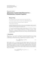
Báo cáo hóa học: "Research Article Signal Classification in Fading Channels Using Cyclic Spectral Analysis" ppt

Hindawi Publishing Corporation
EURASIP Journal on Wireless Communications and Networking
Volume 2009, Article ID 879812, 14 pages
doi:10.1155/2009/879812
Research Article
Signal Classification in Fading Channels Using Cyclic
Spect ral Analysis
Eric Like,
1
Vasu D. Chakravarthy,
2
Paul Ratazzi,
3
and Zhiqiang Wu
4
1
Air Force Institute of Technology, Department of Electrical Engineering, Wright-Patterson Air Force Base,
OH 45433, USA
2
Air Force Research Laboratory, Sensors Directorate, Wright-Patterson Air Force Base, OH 45433, USA
3
Air Force Research Laboratory, Information Directorate, Griffiss Air Force Base, NY 13441, USA
4
Department of Electrical Engineering, Wright State University, Dayton, OH 45435, USA
Correspondence should be addressed to Zhiqiang Wu,
Received 4 May 2009; Accepted 13 July 2009
Recommended by Mischa Dohler
Cognitive Radio (CR), a hierarchical Dynamic Spectrum Access (DSA) model, has been considered as a strong candidate for
future communication systems improving spectrum efficiency utilizing unused spectrum of opportunity. However, to ensure the
effectiveness of dynamic spectrum access, accurate signal classification in fading channels at low signal to noise ratio is essential.
In this paper, a hierarchical cyclostationary-based classifier is proposed to reliably identify the signal type of a wide range of

unknown signals. The proposed system assumes no a priori knowledge of critical signal statistics such as carrier frequency, carrier
phase, or symbol rate. The system is designed with a multistage approach to minimize the number of samples required to make
a classification decision while simultaneously ensuring the greatest reliability in the current and previous stages. The system
performance is demonstrated in a variety of multipath fading channels, where several multiantenna-based combining schemes
are implemented to exploit spatial diversity.
Copyright © 2009 Eric Like et al. This is an open access article distributed under the Creative Commons Attribution License, which
permits unrestricted use, distribution, and reproduction in any medium, provided the original work is properly cited.
1. Introduction
Wireless access technologies have come a long way and are
expected to radically improve the communication environ-
ment. On the other hand, the demand for spectrum usage
in all environments has seen a considerable increase in the
recent years. As a result, novel methods to maximize the
use of the available spectrum have been proposed. One
critical area is through the use of cognitive radio [1, 2].
Traditionally, wireless devices access the spectrum in a
static bandwidth allocation. As the number of wireless users
have increased, there has been a corresponding decrease in
the amount of available spectrum. Cognitive radio seeks
to relieve this burden by determining which areas of the
spectrum are in use at a particular time. If a given band of
the spectrum is not currently being used, that band could
be used by another system. Given the dynamic nature of
the current communication environment, cognitive radio
and dynamic spectrum access has attracted strong interest
in its capability of drastically increasing the spectrum
efficiency. Many spectrum sensing algorithms have been
proposed for cognitive radio, such as energy detection, pilot-
based coherent detection, covariance-based detection, and
cyclostationary detection [3, 4]. Cyclostationary detection-

based spectrum sensing is capable of detecting the primary
signal from the interference and noise even in very low SNR
region [4]. Hence, the FCC has suggested cyclostationary
detectors as a useful alternative to enhance the detection
sensitivity in CR networks.
However, a more efficient method to maximize the use
of the available spectrum would be to not simply avoid
frequency bands that are in use, but rather to limit the
amount of in-band transmission down to an acceptable
low level so as to avoid interfering with the original user.
For example, hybrid overlay/underlay waveforms have been
proposed in [5] to exploit not only unused spectrum bands
2 EURASIP Journal on Wireless Communications and Networking
but also under-used spectrum bands in cognitive radio. Since
different signals are able to tolerate different amounts of
interference, the signal type of the original user will have to
be determined. In this case, merely detecting the presence of
the signal will not be sufficient.
Modulation recognition and signal classification has
been a subject of considerable research for over two decades.
Classification schemes can generally be classified into one
of two broad categories—likelihood-based (LB) approaches
and feature-based (FB) approaches. LB approaches attempt
to provide an optimal classifier by deriving a model for
the signals being considered, and choosing the classification
scheme with the greatest likelihood. However, a complete
mathematical description of the model is usually extremely
complex to arrive at, and generally the systems are highly
sensitive to modeling errors. Additionally, the complexity
of the classifier can frequently become too burdensome to

operate in a real-time manner [6, 7].
FB approaches attempt to extract critical statistics from
the received signal to make a classification based on the
reduced data set. This can frequently be performed at a
fraction of the complexity of LB systems. While FB methods
are suboptimal in the Bayesian sense, they often provide near
optimal performance [8].
FB systems have been implemented using a vast array
of features. These have included statistics derived from
the instantaneous amplitude, phase, and frequency, zero-
crossing intervals, wavelet transforms, amplitude and phase
histograms, constellation shapes, as well as many others [8–
10]. However, many of these methods require a priori knowl-
edge of critical signal statistics, such as the carrier frequency,
carrier phase, symbol rate, or timing offset, among others.
However, these statistics are generally unknown in practical
applications, and requiring their knowledge severely limits
the utility of the classifier.
One area that has demonstrated a considerable amount
of potential is cyclostationary- (CS-) based approaches.
CS methods have been demonstrated to be insensitive
to unknown signal parameters and to preserve the phase
information in the signal [11, 12]. In [13, 14] the Spectral
Coherence Function (SOF) was used to classify lower-order
digital modulation schemes. In [10], mixed second-order
and fourth-order cyclic cumulants (CCs) were used to
distinguish PSK and QAM signals. In [15] sixth- and lower-
order CCs were utilized to classify a wide range of signals,
and in [16] the ability of fourth-order through eighth-order
CCs were investigated to classify QAM, ASK, and PSK signals

of different orders.
However, each of the classifies above was only simulated
in an AWGN channel and most assume knowledge of the
unknown signal’s carrier frequency, phase, or symbol rate.
For a more realistic analysis, classifier performance should be
assessed in fading channels. In [6] the authors investigated
the use of eighth-order CCs to classify digital signals in a
flat fading channel. By employing a multiantenna receiver
using selection combining (SC), the system performance was
shown to increase considerably. However, like the schemes
above, it too assumed prior knowledge of the signal’s
symbol rate, and that the carrier frequency had already been
removed. Additionally, while SC was shown to improve the
performance of the classifier, it does not fully exploit the
multiple received copies of the signal.
In this paper, we extend the results of [6, 14]toinvestigate
the use of cyclic spectral analysis and CCs in a hierarchical
approach for modulation recognition of a wide range of
signals, with no a priori knowledge of the signal’s carrier
frequency, carrier phase, or symbol rate. Specifically, the
proposed classifier will attempt to discriminate between AM,
BFSK, OFDM, CDMA, 4-ASK, 8-ASK, BPSK, QPSK, 8-PSK,
16-PSK, 16-QAM, and 64-QAM modulation types. Multiple
combining methods are investigated and the performance of
the classifier under various channel conditions is assessed.
The classifier features identified in [14] based on the
SOF and in [6] based on eighth-order CCs are used as
a benchmark for comparison purposes. In Section 2 the
underlying statistics are developed, and the cyclostationary
features to be used are defined. In Section 3 the multiantenna

combining schemes to be investigated are described, and the
proposed classifier design is given in Section 4.InSection 5
simulation results are presented, followed by a conclusion in
Section 6.
2. Signal Statistic Development
2.1. Signal Model. A modulated signal as received by the
classifier can be modeled as
y
(
t
)
= s
(
t −t
0
)
e
j2πf
c
t
e
jφ
+ n
(
t
)
,(1)
where
y(t) is the complex-valued received signal, f
c

is the
carrier frequency, φ is the carrier phase, t
0
is the signal time
offset, n(t) is additive Gaussian noise, and s(t) denotes the
time-varying message signal. For digital signals, this can be
further specified as
y
(
t
)
= e
j2πf
c
t
e
jφ
∞

k=−∞
s
k
p
(
t −kT
s
−t
0
)
+

n
(
t
)
,(2)
where p(t) is the pulse shape, T
s
is the symbol period, and s
k
is the digital symbol transmitted at time t ∈ (kT −T/2, kT +
T/2). Here, the symbols s
k
are assumed to be zero mean,
identically distributed random variables.
CS-based features have been used in numerous ways
as a reliable tool to determine the modulation scheme of
unknown signals [10, 14, 16]. CS-based approaches are
based on the fact that communications signals are not accu-
rately described as stationary, but rather more appropriately
modeled as cyclostationary. While stationary signals have
statistics that remain constant in time, the statistics of CS
signals vary periodically. These periodicities occur for signals
of interest in well defined manners due to underlying period-
icities such as sampling, scanning, modulating, multiplexing,
and coding. This resulting periodic nature of signals can
be exploited to determine the modulation scheme of the
unknown signal.
EURASIP Journal on Wireless Communications and Networking 3
2.2. Second-Order Cyclic Features. The autocorrelation func-
tion of a CS signal x(t) can be expressed in terms of its

Fourier Series components [11, 12]:
R
x
(
t, τ
)
= E

x
(
t + τ/2
)
x
∗
(
t
−τ/2
)

=

{α}
R
α
x
(
τ
)
e
j2παt

,(3)
where E
{·} is the expectation operator, {α} is the set of
Fourier components, and the function R
α
x
(τ) giving the
Fourier components is termed the cyclic autocorrelation
function (CAF) given by
R
α
x
(
τ
)
= lim
T →∞
1/T

T/2
−T/2
R
x
(
t, τ
)
e
−j2παt
.
(4)

Alternatively, in the case when R
x
(t, τ) is periodic in t with
period T
0
,(4) can be expressed as
R
α
x
(
τ
)
= 1/T
0

T
0
/2
−T
0
/2
R
x
(
t, τ
)
e
−j2παt
.
(5)

The Fourier Transform of the CAF, denoted the Spectral
Correlation Function (SCF), is given by
S
α
x

f

=

∞
−∞
R
α
x
(
τ
)
e
−j2πfτ
dτ.
(6)
This can be shown to be equivalent (assuming cyclo-
ergodicity) to [11]
S
α
X

f


=
lim
T →∞
lim
Δt →∞
1
Δt

Δt/2
−Δt/2
1
T
X
T

t, f +
α
2

X
∗
T

t, f −
α
2

dt,
(7)
X

T

t, f

=

t+T/2
t
−T/2
x
(
u
)
e
j2πfu
du
. (8)
Here it can be seen that S
α
x
is in fact a true measure of
the correlation between the spectral components of x(t). A
significant benefit of the SCF is its insensitivity to additive
noise. Since the spectral components of white noise are
uncorrelated, it does not contribute to the resulting SCF for
any value of α
/
=0. This is even the case when the noise
power exceeds the signal power, where the signal would be
undetectable using a simple energy detector. At α

= 0, where
noise is observed, the SCF reduces to the ordinary Power
Spectral Density (PSD).
To derive a normalized version of the SCF, the Spectral
Coherence Function (SOF) is given as
C
α
X

f

=
S
α
X

f


S
0
X

f + α/2

∗
S
0
X


f −α/2


1/2
. (9)
The SOF is seen to be a proper coherence value with a
magnitude in the range of [0, 1]. To account for the unknown
phase of the SOF, the absolute value of C
α
X
( f )iscomputed
and used for classification. The SOFs of some typical
modulation schemes are shown in Figures 1 and 2. The SOF
of each modulation scheme generates a highly distinct image.
Theseimagescanthenbeusedasspectralfingerprintsto
identify the modulation scheme of the received signal.
−0.5
0
0.5
0
0.2
0.4
0.6
0.8
1
0
0.5
1
1.5
Cycle frequency α (Fs)

Spectral frequency f (Fs)
Figure 1: SOF of a BPSK signal in an AWGN Channel at 5 dB SNR,
with 1/Ts
= Fs/10, Fc = 0.25 Fs, no. of samples = 4096.
−0.5
0
0.5
0
0.2
0.4
0.6
0.8
1
0
0.5
1
1.5
Cycle frequency α (Fs)
Spectral frequency f (Fs)
Figure 2: SOF of a BFSK signal in an AWGN Channel at 5 dB SNR,
with 1/Ts
= Fs/10, Fc = 0.25 Fs, no. of samples = 4096.
An additional benefit to using the SOF is its insensitivity
to channel effects. Wireless signals are typically subject to
severe multipath distortion. Taking this into consideration,
the SCF of a received signal is given as
S
α
Y


f

= H

f +
α
2

H
∗

f −
α
2

S
α
x

f

, (10)
y
(
t
)
= x
(
t
)

⊗h
(
t
)
,
(11)
where h(t) is the unknown channel response, and H(f )
is the Fourier Transform of h(t). Here it can be seen that
the resulting SCF of the received signal can be significantly
distorted depending on the channel. However, when forming
the SOF, by substituting (10) into (9) it is evident that the
channel effects are removed, and the resulting SOF is equal
to that of the original undistorted signal [12]. As a result, the
SOF is preserved as a reliable feature for identification even
when considering propagation through multipath channels,
so long as no frequency of the signal of interest is completely
4 EURASIP Journal on Wireless Communications and Networking
−0.5
0
0.5
0
0.2
0.4
0.6
0.8
1
0
0.5
1
1.5

Cycle frequency α (Fs)
Spectral frequency f (Fs)
Figure 3: SOF of a BPSK signal in a Multipath Fading Channel at
5 dB SNR, with 1/Ts
= Fs/10, Fc = 0.25 Fs, no. of samples = 4096.
0
0.5
0
0.2
0.4
0.6
0.8
1
0
0.5
1
1.5
−0.5
Cycle frequency α (Fs)
Spectral frequency f (Fs)
Figure 4: SOF of a BFSK signal in a Multipath Fading Channel at
5 dB SNR, with 1/Ts
= Fs/10, Fc = 0.25 Fs, no. of samples = 4096.
nullified by the channel. The SOFs of some typical signals
undergoing multipath fading are shown in Figures 3 and 4.
To compute the SOF for a sampled signal, a sliding
windowed FFT of length N can be used to compute X
T
,and
a sum taken over the now discrete versions of X

T
gives the
resulting equation for S
α
X
( f ). Additionally, the limits in (7)
and (8) must be made finite, and an estimate of the SCF is
obtained. This has the effect of limiting the temporal and
spectral resolution of the SCF. In (7), Δt is the amount of
time over which the spectral components are correlated. This
limits the temporal resolution of the signal to Δt.In[17] the
cyclic resolution is shown to be approximately Δα
= 1/Δt.
Similarly, the spectral resolution is limited to Δ f
= 1/T,
where 1/T is the resolution of the FFT used to compute X
T
.
To obtain a reliable estimate of the SCF, the random
fluctuations of the signal must be averaged out. The resulting
requirement is that the time-frequency resolution product
must be made very large, with ΔtΔ f
 1, or equivalently,
Δ f
 Δα. This has the effect of requiring a much finer
resolution for the cycle frequencies than would be provided
by the FFT operation. To compensate for this, it has been
proposed to zero pad the input to the FFTs out to the full
length of the original signal [14]. However, this leads to
a computationally infeasible task. A more suitable method

is to first estimate the cycle frequencies of interest using
the method outlined in [18]. After the appropriate cycle
frequencies have been located, the SCF can be computed
using the equivalent method of frequency smoothing on the
reduced amount of data:
S
α
X

f

=
1
Δ f

f +Δ f/2
f
−Δ f/2
X
Δt

t, f +
α
2

X
∗
Δt

t, f −

α
2

dt
, (12)
where X
Δt
(t, f )isdefinedin(8)withT replaced by Δt.
The resulting feature derived from the SOF is a three-
dimensional image. This presents an unreasonable amount
of data for a classifier to operate on in real time. Therefore, it
must be further reduced to provide a more computationally
manageable feature. In [14] the authors proposed using
merely the cycle frequency profile of the SOF. However, in
our previous work of [13] it was demonstrated that with
a minimal increase in computational complexity, both the
frequency profile as well as the cycle frequency profile can be
used, creating a pseudo-three-dimensional image of the SOF
which performs at a significantly higher degree of reliability
for classification. The resulting feature used for classification
is then defined as the cycle frequency profile:
−→
α = max
f

C
α
X

(13)

and the spectral frequency profile
−→
f = max
α

C
α
X

. (14)
These features can then be analyzed using a pattern
recognition-based approach. Due to its ease of implemen-
tation, and its ability to generalize to any carrier frequency
or symbol rate, a neural network-based system is proposed
to process the feature vectors. This system will be outlined in
Section 4.
2.3. Higher-Order Cyclic Features. While the SOF produces
highly distinct images for different modulation schemes,
some modulation schemes (such as different orders of
a single modulation scheme) produce identical images.
Therefore, while the SOF is able to reliably classify each of
the analog signals as well as classify the digital schemes into a
modulation family, it will not be able to distinguish between
some digital schemes (namely, QAM and M-PSK, M>4),
or determine the order of the modulation. As an example
of this, compare the estimated SOF of the BPSK signal in
Figure 1 with that of a 4-ASK signal shown in Figure 5.
To discriminate between signals of these types, higher-
order cyclic statistics (HOCSs) must be employed. For
this end, we introduce the nth-order/q-conjugate temporal

moment function:
R
x
(
t, τ
)
n,q
= E
⎧
⎨
⎩
i=n

i=1
x
(∗)
i
(
t + τ
i
)
⎫
⎬
⎭
, (15)
EURASIP Journal on Wireless Communications and Networking 5
0
0
0.2
0.4

0.6
0.8
1
0.5
0
0.5
1
1.5
−0.5
Cycle f
requency α (Fs)
Spectral frequency f (Fs)
Figure 5: SOF of a 4-ASK signal in an AWGN Channel at 5 dB SNR,
with 1/Ts
= Fs/10, Fc = 0.25 Fs, no. of samples = 4096.
where (∗) represents the one of q total conjugations. For the
case of n
= 2, q = 1, τ
1
= τ/2, and τ
2
=−τ/2, the TMF
reduces to the autocorrelation function defined in (3). Like
the autocorrelation function, the TMF of CS signals exhibits
one or more periodicities and can be expressed in terms of its
Fourier coefficients:
R
x
(
t, τ

)
n,q
=

{α}
R
α
x
(τ)
n,q
e
j2παt
,
R
α
x
(τ)
n,q
= lim
T →∞
1/T

T/2
−T/2
R
x
(
t, τ
)
n,q

e
−j2παt
,
(16)
where R
α
x
(τ)
n,q
is termed the cyclic temporal moment
function.
To isolate the cyclic features present at an order n from
those made up of products of lower-order features we make
use of the nth-order/q-conjugate temporal cumulant (TC).
The TC is given by the moment to cumulant formula
C
x
(t, τ)
n,q
= Cum

x
(∗)
1
(
t + τ
1
)
···x
(∗)

n
(
t + τ
n
)

=

{P
n
}
(−1)
Z−1
(
Z
−1
)
!
Z

z=1
m
x
(t, τ
z
)
n
z
,q
z

,
(17)
where
{P
n
} is the set of distinct partitions of {1, 2, ,n},
τ
z
is a delay vector with indices specified by z,andn
z
and
q
z
correspond to the number of elements and the number
of conjugated terms in the subset P
z
,respectively.When
computing the TC, the effect of lower-order moments is
effectively subtracted off, leaving the only remaining impact
due to the current order. The TC is also a periodic function
for cyclostationary signals, with its Fourier components
given by
C
γ
x
(τ)
n,q
= lim
T →∞
1/T


T/2
−T/2
C
x
(t, τ)
n,q
e
−j2πγt
,
(18)
where C
γ
x
(τ) is the cyclic cumulant (CC) of x(t).
Since it is computationally infeasible to perform a multi-
dimensional Fourier Transform of (18) to compute a higher-
order variation of the SCF, we are restricted to manipulate
(18) directly as a feature for classification. However, by
substituting (2) into (17)and(18), it can be shown that the
resulting value of the CC is given by [6]
C
γ
x
(τ)
n,q
= C
s
,n,q
T

−1
s
e
−j2πβt
0
e
j
(
n−2q
)
φ
e
j2πf
c

n−1
u
=1
(−)
u
τ
u
×

∞
−∞
p
(∗)
n
(

t
)
u=n−1

u=1
p
(∗)
n
(
t + τ
u
)
e
−j2πβ
dt,
γ
= β +

n − 2q

f
c
, β =
k
T
s
,
(19)
where C
s

,n,q
is the nth-order/q-conjugate cumulant of the
stationary discrete data sequence, and the possible minus
sign, (
−)
u
, comes from one of the q conjugations (∗)
n
.Thus,
the resulting value of the CC of the received signal is directly
proportional to C
s
,n,q
. The value of C
s
,n,q
is well known for
common modulation schemes and is given in Ta bl e 1 [6].
As in the case of the SOF, the magnitude of (19)istaken
to remove the phase dependence on the carrier frequency,
phase, and signal time offset. The resulting feature is given as
Γ
y
(γ, τ)
n,q
=







C
s,n,q
T
−1
s
×

∞
−∞
p
(∗)
n
(
t
)
u=n−1

u=1
p
(∗)
n
(
t + τ
u
)
e
−j2πβ
dt







γ = β +

n − 2q

f
c
, β =
k
T
s
.
,
(20)
Assuming a raised cosine pulse shape, the maximum of
the resulting function Γ
y
(γ, τ)
n,q
has been shown to occur
at τ
=
−→
0
n

,where
−→
0
n
is an n-dimensional zero vector.
Furthermore, at τ
=
−→
0
n
, the function decreases with
increasing k [6]. k is therefore chosen to be 1 to maximize
the test statistic. Γ
y
(γ, τ)
n,q
should then be evaluated at γ =
1/T
s
+(n − 2q) f
c
.
Thedesiredvalueofγ used to evaluate the CC depends
on both f
c
and 1/T
s
, which are both unknown and will
need to be estimated. This value of γ can be derived by
noting that cyclic features will only occur at intervals of

1/T
s
. For a raised cosine pulse, the magnitude of Γ
y
(γ, τ)
n,q
obtains its largest value at k = 0, corresponding to a cycle
frequency of γ
= (n − 2q) f
c
. The next largest peak occurs
at k
= 1, which is the desired cycle frequency. To estimate
the desired value of γ, all that is needed is to search for the
cycle frequency corresponding to the largest cyclic feature,
and evaluate the CC at an offset of 1/T
s
from this location.
Given that the variance of the CC estimates increase with
increasing order [16], we desire to use the lowest order
CC possible to estimate 1/T
s
to achieve a more reliable
estimate. The second-order/one-conjugate CC is therefore
selected to estimate 1/T
s
, as all of the modulation schemes
6 EURASIP Journal on Wireless Communications and Networking
Table 1: Theoretical stationary cumulants [6].
C

s
,n,q
4-ASK 8-ASK BPSK Q-PSK
C
s
,2,0
111 0
C
s
,2,1
111 1
C
s
,4,0
−1.36 −1.24 −21
C
s
,4,1
−1.36 −1.24 −20
C
s
,4,2
−1.36 −1.24 −2 −1
C
s
,6,0
8.32 7.19 16 0
C
s
,6,1

8.32 7.19 16 -4
C
s
,6,2
8.32 7.19 16 0
C
s
,6,3
8.32 7.19 16 4
C
s
,8,0
−111.85 −92.02 −272 −34
C
s
,8,1
−111.85 −92.02 −272 0
C
s
,8,2
−111.85 −92.02 −272 34
C
s
,8,3
−111.85 −92.02 −272 0
C
s
,8,4
−111.85 −92.02 −272 −34
C

s
,n,q
8-PSK 16-PSK 16-QAM 64-QAM
C
s
,2,0
000 0
C
s
,2,1
111 1
C
s
,4,0
00−0.68 −0.62
C
s
,4,1
000 0
C
s
,4,2
−1 −1 −0.68 −0.62
C
s
,6,0
000 0
C
s
,6,1

0 0 2.08 1.80
C
s
,6,2
000 0
C
s
,6,3
4 4 2.08 1.80
C
s
,8,0
10−13.98 −11.50
C
s
,8,1
000 0
C
s
,8,2
00−13.98 −11.50
C
s
,8,3
000 0
C
s
,8,4
−33 −33 −13.98 −11.50
being considered will contain a feature at this cycle frequency.

Using the value of γ
= 1/T
s
computed from the second-order
CC, paired with the estimate of γ
= (n − 2q) f
c
obtained for
each CC, the computation of the value of γ
= 1/T
s
+(n−2q) f
c
is straightforward.
The resulting values of the different order/conjugate pairs
of the CCs can now be used to classify the signal further to
discriminate between signals for which the SOF was unable.
By referring to Ta b le 1 , the specific modulation type as well
as its order can be determined from the expected values of
C
s
,n,q
.In[6] it was proposed to use only the eighth-order CCs
of the received signal. However, the results can be improved
by using the lower-order CCs in the estimate, whose variance
is shown to be less than that of corresponding higher orders.
By implementing a hierarchical scheme, lower-order CCs can
perform an initial classification, followed by progressively
higher-order CCs to further refine the classification decision.
In this way a more reliable estimate can be obtained.

Furthermore, in poor channel conditions, the hierarchical
scheme is expected to better distinguish between modulation
families than a scheme based purely on a single-higher order
CC, due to the lower variance in the CCs.
2.4. Identification of OFDM Signals. In an OFDM system, the
subcarriers can be appropriately modeled as independently
modulated signals which exhibit their own second-order
cyclostationary statistics (SOCSs). However, the fact that
their bandwidths overlap reduces the total amount of
observed spectral coherence (SOF) due to the “destruc-
tive interference” between the overlapping cyclostationary
features. As the length of the cyclic prefix used in the
OFDM system is shortened, the observed features in the
SOF are also decreased. In the case where an OFDM
signal is generated without a cyclic prefix, the remaining
cyclostationary features are severely diminished [19]. While
research has shown that cyclostationary features can be
artificially introduced into a transmitted OFDM signal by
transmitting correlated data on selected subcarriers [20],
in the absence of these intentionally designed phenomena
the cyclic features present in a received OFDM signal will
EURASIP Journal on Wireless Communications and Networking 7
0
0
0.2
0.4
0.6
0.8
1
0.5

0
0.5
1
1.5
−0.5
Cycle frequency α (Fs)
Spectral frequency f (Fs)
Figure 6: SOF of a QPSK signal in an AWGN Channel at low (0 dB)
SNR,with1/Ts
= Fs/10, Fc = 0.25 Fs, no. of samples = 4096.
0
0
0.2
0.4
0.6
0.8
1
0.5
0
0.5
1
1.5
−0.5
Cycle frequency α (Fs)
Spectra
l frequency f (Fs)
Figure 7: SOF of an OFDM signal in an AWGN Channel at low
(0 dB) SNR, with 32 subcarriers, subcarrier spacing ΔF
= Fs/10, Fc
= 0.25 Fs, no. of samples = 4096.

generally be very weak and difficult to detect. In the presence
of low SNR, the difference between the SOF of OFDM signals
with no cyclic prefix and that of single carrier QAM and
MPSK signals (M>2) becomes negligible. As an example,
refer to Figures 6 and 7 depicting the SOF of a QPSK signal
and OFDM signal, respectively, generated at an SNR of 0 dB.
While the existence of cyclic prefix in OFDM signal
makes the detection and classification of OFDM signal much
easier, in reality the signal detector/classifier sometimes
needs to make decision in a short observation time window.
When this observation window is shorter than the duration
of one OFDM symbol, cyclic prefix is not included in
the observation window. Hence, since there are numerous
efficient algorithms to detect and classify an OFDM signal
based on its cyclic prefix through the use of a simple
autocorrelation procedure [21–23], we focus on the case of
an OFDM signal transmitted with no cyclic prefix. Therefore,
an intermediate stage is needed between the SOF-based
classifications and the HOCS-based classifications.
A simple yet effective method to distinguish OFDM
signals from the single carrier signals in question is obtained
by considering the fact that OFDM signals are composed of
multiple independently time varying signals. By use of the
Central Limit Theorem from probability theory, these can
be approximated as a Gaussian random signal [21]. Through
the use of a simple Gaussianity test, the OFDM signals can
therefore be accurately identified. Since Gaussian signals do
not exhibit features for CCs other than their 2nd-order/1-
conjugate CC, the CC features derived above to distinguish
between the HOCS features can also be used to classify an

OFDM signal, assuming the number of subcarriers present is
high.
3. Multiantenna Combining
In the presence of multipath fading channels, the received
signal can be severely distorted. Several methods exist to
exploit spacial diversity through the use of multiple receiver
antennas. By assuming that the channel fades independently
on each antenna, the signal received on each can be
combined in various ways to improve performance. The
general equation for the received analytic signal undergoing
multipath propagation is given by
y
(
t
)
=
P

p=1
κ
p
e
jθ
p
x

t − t
p

+ n

(
t
)
, (21)
where κ
p
e
θ
p
is the channel response on path p, t
p
is the delay
of the pth path, and P is the total number of paths received
by the classifier.
This can be separated into two general situations. In the
first situation, the channel is varying sufficiently slowly so
that it can be assumed to be static over the block of data being
analyzed.
If the signal is assumed to only be experiencing flat
fading, the simplest combining method is to employ a selec-
tion combiner (SC). In [6], the effectiveness of an SC-based
system was evaluated to combat the effects of flat fading for
modulation recognition. By estimating the received power
on each antenna, the signal on the antenna with the highest
observed power can be selected for classification, while the
others are discarded. When assuming that the noise on each
antenna has identical powers, this choice will correspond to
the signal with the largest SNR, which leads to an extremely
simple implementation.
However, in the case of flat fading, a maximum ratio

combiner (MRC) can also be implemented. In this case,
the signal received from each antenna is weighted by its
SNR before being summed with the signals from the other
antennas. In practice, the value of the SNR can be estimated
simply by using one of several methods [24–26]. However,
for the signals to combine coherently, the unknown phase
on each channel must be compensated for before adding
8 EURASIP Journal on Wireless Communications and Networking
them together. This can be performed by computing the
correlation between signals from two channels given by
E


y
1
(
t
)
y
∗
2
(
t
)

=
E

κ
1

e
jθ
1
x
(
t
)
+ n
1
(
t
)

×

κ
∗
2
e
−jθ
2
x
∗
(
t
)
+
n
∗
2

(
t
)

=
σ
2
x
κ
1
κ
2
e
j(θ
1
−θ
2
)
,
(22)
where σ
2
x
is the power of the signal to be classified. From
here, the relative phase difference is given as the phase of the
resulting statistic:
Δ

θ = ∠


σ
2
x
κ
1
κ
2
e
j
(
θ
1
−θ2
)

. (23)
The signal
y
2
(t) can then be multiplied by e
jΔ

θ
to align
its phase with the phase of the first channel. This procedure
can be repeated as necessary depending on the number of
antennas employed.
An additional method to compensate for channel cor-
ruption in the SOF computation is through a variant of the
MRC. While the SOF was derived to be highly insensitive to

channel distortion in (10), the SOF image obtained when a
deep fade can be significantly distorted by the additive noise
components present, which will be amplified when forming
the SOF from the SCF. The MRC variant described here
then attempts to compensate for this effect by combining
weighted estimates of the SOF from each receiver. For this
method, the SOF is computed independently for the signal
received on each antenna. After the feature vectors
−→
α and
−→
f are formed, they are each weighted by the SNR estimated
on their respective antennas. Then each is summed, and
the procedure follows as before. It is worth noting that this
method can be utilized in any fading channel, without the
necessity for the assumption of a flat fading channel.
The second general situation exists when the channel
is not varying slow enough to be approximated as static
throughout the signal’s evaluation. Since each of the classifi-
cation methods above attempts to estimate expected values of
joint moments, they are quickly corrupted by a rapidly fading
channel. The HOCS features are particularly sensitive since
they require a greater amount of samples to converge, during
which time the channel can vary drastically. The first stage
SOF-based classifier is less sensitive to channel variations,
thus providing greater incentive for its use as the first stage
in the system.
4. Classifier Design
The proposed classifier is designed to classify AM, BFSK,
OFDM, DS-CDMA, 4-ASK, 8-ASK, BPSK, QPSK, 8-PSK,

16-PSK, 16-QAM, and 64-QAM modulation types. It is
designed in a hierarchical approach to classify the signals
using the smallest amount of required data possible, while
simultaneously maximizing the reliability of the system. At
each stage in the system, the signal’s modulation scheme is
either classified or grouped with similar schemes narrowed
down into a smaller subset. The system is designed to require
no knowledge of the received signal’s carrier frequency, phase
shift, or symbol rate, and only assumes that the signal’s
presence has been identified, and that it is located within the
bandwidth of interest.
The first stage of the classifier computes the SOF of
the signal by (i) using the SSCA method outlined in [18]
to estimate the cycle frequencies of interest, (ii) applying
(12)followedby(9) to compute the SOF of the received
signal, and (iii) compressing the data into the feature vector
composed of the concatenation of
−→
α and
−→
f .Asmentioned
in Section 2.2, the feature vector is analyzed by a neural
network-based system. Neural networks were chosen due
to their relative ease of setup and use as well as its ability
to generalize to any carrier frequency or symbol rate. The
system consists of five independent neural networks, each
trained to classify a signal as either AM, BFSK, DS-CDMA, or
a linear modulation scheme with a real-valued constellation
(BPSK, 4-ASK, 8-ASK) or a complex-valued constellation
(OFDM, 8-PSK, 16-PSK, 16-QAM, 64-QAM). Each network

has four neurons in their hidden layer and one neuron
in the output layer, each layer with a hyperbolic tangent
sigmoid transfer function. The inputs to each network are
the concatenated profile vectors. A system diagram for this
first stage is given in Figure 8.
The BPSK and ASK signals demonstrate identical SOF
images and are not distinguishable based on that metric
alone. Similarly, the PSK and QAM signals have identical
spectral components. As mentioned in the previous section,
the OFDM signal is composed of potentially independently
varying signals on each subchannel, which may or may not
demonstrate SOCS. However, due to the overlapping nature
of the subchannels in an OFDM system, the resulting SOF is
decreased, resulting in an SOF image that resembles those of
QAM and PSK signals. Additionally, the DS-CDMA scheme
can be thought to look like a BPSK signal. However, due to
the underlying periodicities incurred by both its symbol rate
as well as its spreading code, it produces features not found
in BPSK or QPSK signals. Thus it can be reliably classified
by its SOF image without knowledge of its spreading
code.
The HOCS-based processing is also implemented in a
hierarchical approach to maximize the ability to accurately
determine the class of a signal before further narrowing the
list of candidate modulations. This is a critical step since
the variance of the CC estimates increases with increasing
order [16]. Therefore, we attempt to classify a signal using the
lowest order CC possible before proceeding to higher-order
CCs.
In each stage, the feature vector used for classification

is composed of the appropriate CCs estimated from the
received signal:

Ψ =

Γ
y

1
T
,
−→
0
n

n,q
1
, , Γ
y

1
T
,
−→
0
n

n,q
k


, (24)
where n and q
j
refer to the appropriate order and number
of conjugations for the stage. This vector is then compared
EURASIP Journal on Wireless Communications and Networking 9
SOF
Max
BFSK
network
CDMA
network
AM
network
BPSK
network
QAM/PSK/
OFDM
network
x(t)
−→
f ,
−→
αz= arg(max
k
(y
k
))
y
1

∈ [−1, 1]
y
2
∈ [−1, 1]
y
3
∈ [−1, 1]
y
4
∈ [−1, 1]
y
5
∈ [−1, 1]
Figure 8: SOF system diagram.
to the expected vector obtained for each modulation type,
defined similarly as
Ψ
(i)
=

Γ
(
i
)

1
T
,
−→
0

n

n,q
1
, , Γ
(
i
)

1
T
,
−→
0
n

n,q
k

, (25)
where i corresponds to one of the M possible modulation
schemes being considered by the current stage. The class
corresponding to the feature vector with the minimum
Euclidean distance from the estimated vector is selected. The
processing is then handed off to the next stage until the final
modulation scheme as been determined.
The network diagram of the system is shown in Figure 9.
If the SOF network determined the signal to have a real-
valued modulation scheme (BPSK, 4-ASK, 8-ASK), then it
is handed off to the final classification stage using eighth-

order CCs. Otherwise, the fourth-order CCs are used to
classify the signal as being an OFDM signal or as having
either a circular constellation (8-PSK, 16-PSK) or a square
constellation (QPSK, 16-QAM, 62-QAM). For each signal
class, the final stage of the classifier forms the feature vector

Ψ from the five eighth-order CCs of the received signal,
except for OFDM signals which were already identified using
fourth-order CCs.
5. Simulation Results
Simulations were run with AM, BFSK, OFDM, DS-CDMA,
4-ASK, 8-ASK, BPSK, QPSK, 8-PSK, 16-PSK, 16-QAM, and
64-QAM modulated signals. Each of the digital signals was
simulated with an IF carrier frequency uniformly distributed
between 0.23 and 0.27 times the sampling rate, a symbol
rate uniformly distributed between 0.16 and 0.24 times the
sampling rate, and a raised cosine pulse shape with a 50%
excess bandwidth, with the exception of the BFSK which was
modeled with a rectangular pulse shaping filter. The OFDM
signal employed 32 subcarriers using BPSK modulation
(without a cyclic prefix), and like the other digital signals
was passed through a raised cosine filter with a 50% excess
bandwidth. The analog signals were also bandlimited using
the same raised cosine filter. Additionally, the classifier’s
receive filter is assumed to be an ideal low-pass filter. Since
the symbol rate is assumed to be unknown, the digital signals
were not sampled at an integer multiple of the symbol rates,
but were sampled at a constant rate independent of the
symbol rate and the IF carrier frequency.
The first stage of the classifier used 4096 received time

samples, corresponding to an average of approximately 410
symbols, to compute the SOF estimate of the signal, and
used this estimate in the neural-network system. The HOCS-
based system was tested with 65 536 samples for its classifica-
tion decision, corresponding to an average of approximately
6500 symbols. The system was tested in a variety of channel
conditions, with an SNR range of 0 dB to 15 dB. The
channel models simulated include a flat fading channel, two-
path fading channel, and a harsh 20-path fading channel.
Each of the fading channels implemented used independent
equal-power paths with Rayleigh distributed amplitudes and
uniformly distributed phases. The channels are simulated for
two distinct fading scenarios:
(1) slow fading such that the channel can be approxi-
mated as constant over the block of observed data;
(2) fast fading with each path maintaining a coherence
value of 0.9 over 500 samples, approximately equal to
50 symbols.
Additionally, it is assumed that the SNR of the signal
on each antenna can be accurately estimated, and that
the channel phase offsetbetweenantennasisaccurately
determined for the slow flat fading channel.
The system performance is measured by its probability
of correct classification (Pcc), defined as the percentage of
the total number of modulation classifications made that
were accurate. The SOF-based classifier from [14] using only
the cycle frequency profile is simulated as a benchmark for
comparison to the first stage of the proposed classifier. This
demonstrates the advantage of using both the cycle frequency
as well as the spectral frequency profile for the initial

classification stage. The purely eighth-order CC feature
vector from [6] is used as a benchmark for comparison to the
proposed classifier from end to end. However, to achieve a
fair comparison, the AM, DS-CDMA, and BFSK signals were
10 EURASIP Journal on Wireless Communications and Networking
AM
BFSK
CDMA
OFDM
Real-valued
constellation
Square
constellation
Circular
constellation
Complex-valued
constellation
4ASK
SOF
C
S,8,0
C
S,8,1
C
S,8,2
C
S,8,3
C
S,8,4
C

S,8,0
C
S,8,1
C
S,8,2
C
S,8,3
C
S,8,4
C
S,8,0
C
S,8,1
C
S,8,2
C
S,8,3
C
S,8,4
BPSK
8ASK
C
S,4,0
C
S,4,1
C
S,4,2
QPSK
16QAM
64QAM

8PSK
16PSK
x
(t)
Figure 9: Proposed system diagram.
excluded from consideration for this case since the purely
eighth-order CC does not have the ability to classify signals
of this type.
The systems were first tested in a slow flat fading channel.
Here, the systems were simulated using a multiantenna
approach. The initial SOF-based stage used the MRC-
variant method outlined in Section 3, while the HOCS-
based stage utilized traditional MRC. Figure 10 compares the
performance of the first stage of the proposed classifier with
that of its benchmark. As can be readily seen, the proposed
classifier obtains a significant performance increase over the
baseline. The initial stage of the proposed classifier achieves
the remarkably high rate nearly 100% Pcc for all SNR levels
of interest when using four antennas with the MRC variant.
Figure 11 compares the final classification performance of
the proposed classifier to its eighth-order CC counterpart. In
this case, the proposed classifier achieves a gain of 3 dB SNR
over the benchmark. It is also noteworthy that as pointed
out in [6], with the addition of only a single antenna, a
considerable performance gain is achieved.
Next, the systems were tested in a two path as well as
a 20-path slow fading channel. As mentioned earlier, the
fading channel is assumed to be static over the duration of
the observation. Here, the initial SOF-based stage was again
implemented with the MRC variant, while the HOCS-based

systems used SC. The performance of the initial classification
stage subject to the two-path channel is shown in Figure 12
and the results under the 20-path channel are shown in
Figure 13. These figures demonstrate the robustness of the
SOF against multipath channel effects, as it is subject to only
0 5 10 15
0.5
0.55
0.6
0.65
0.7
0.75
0.8
0.85
0.9
0.95
1
SNR (dB)
Classification performance
Proposed system-4 antenna
Proposed system-2 antennas
Proposed system-1 antennas
Benchmark system-4 antenna
Benchmark system-2 antennas
Benchmark system-1 antennas
Figure 10: Classification performance of proposed initial SOF-
based classification stage and benchmark in a slow flat fading
channel using the MRC-variant combining scheme.
a slight performance degradation as compared to the flat
fading channel.

The performance of the final classification decision is
shown in Figure 14 for the two-path case and in Figure 15
EURASIP Journal on Wireless Communications and Networking 11
0 5 10 15
0
0.1
0.2
0.3
0.4
0.5
0.6
0.7
0.8
0.9
1
SNR (dB)
Classification performance
Proposed system-4 antenna
Benchmark system-4 antenna
Proposed system-2 antenna
Benchmark system-2 antenna
Proposed system-1 antenna
Benchmark system-1 antenna
Figure 11: Final classification performance of proposed classifier
and benchmark in a slow flat fading channel using MRC.
0 5 10 15
0.5
0.55
0.6
0.65

0.7
0.75
0.8
0.85
0.9
0.95
1
SNR (dB)
Classification performance
Proposed system-4 antenna
Proposed system-2 antennas
Proposed system-1 antennas
Benchmark system-4 antenna
Benchmark system-2 antennas
Benchmark system-1 antennas
Figure 12: Classification performance of proposed initial SOF-
based classification stage and benchmark in a slow two-path fading
channel using the MRC-variant combining scheme.
for the multipath case. The performance of each system is
significantly degraded from the performance under the flat
fading channel. The performance is insufficient to classify a
signal with any reasonable degree of reliability. However, a
benefit to the multistage approach is that it utilizes lower-
order CCs in each decision stage, thus lowering the variance
of the estimated statistic. While this does not achieve a
significant benefit in the final classification stage, it does
allow for a more reliable estimate of the family of the
signal. This is demonstrated in Figures 16 and 17 where the
0 5 10 15
0.5

0.55
0.6
0.65
0.7
0.75
0.8
0.85
0.9
0.95
1
SNR (dB)
Classification performance
Proposed system-4 antenna
Proposed system-2 antennas
Proposed system-1 antennas
Benchmark system-4 antenna
Benchmark system-2 antennas
Benchmark system-1 antennas
Figure 13: Classification performance of proposed initial SOF-
based classification stage and benchmark in a slow 20-path fading
channel using the MRC-variant combining scheme.
ability of the two systems to classify the received signal as
having a real-valued constellation (BPSK, 4ASK, or 8ASK), a
square-constellation (QPSK, 16QAM, or 64 QAM), a circular
constellation (8PSK or 16PSK), or as being an OFDM signal,
where the other three signal types are not considered as
the purely eighth-order CC feature vector is not capable of
classifying them. Here, while it is noted that the number of
antennas used does not affect the overall modulation-family
classification performance, using the multistage approach

does increase the observed classification performance by
approximately two to three times.
Finally, the classifier performance was evaluated under
the faster fading channels. The performance of the SOF-
based classifier is given in Figures 18 and 19. Again, this
initial stage of the classifier is only moderately degraded.
Furthermore, while each classifier is unable to reliably
determine the exact modulation scheme of the received
signal under these harsh channel conditions, the multistage
approach is still able to reliably determine the modulation
family of the signal of interest. The system performance
under the fast varying flat and 20-path channels are shown
in Figures 20 and 21.
The ability of the system to still achieve a high degree of
reliability in determining the modulation family is in part
due to the insensitivity of the SOF to the multipath affect as
well as to the fewer number of required symbols that must
be observed before a classification can be made. Since this
stage of the classifier requires significantly fewer observed
symbols to make a classification, it is only moderately
affected. While the purely eighth-order CC-based classifier
is drastically degraded, the proposed classifier is still able to
produce a moderate gain in modulation class recognition,
demonstrating the ability of the lower-order cumulants to
12 EURASIP Journal on Wireless Communications and Networking
0 5 10 15
0
0.1
0.2
0.3

0.4
0.5
0.6
0.7
0.8
0.9
1
SNR (dB)
Classification performance
Proposed system-4 antenna
Benchmark system-4 antenna
Proposed system-2 antenna
Benchmark system-2 antenna
Proposed system-1 antenna
Benchmark system-1 antenna
Figure 14: Final classification performance of proposed classifier
and benchmark in a slow two-path fading channel using SC.
0 5 10 15
0
0.1
0.2
0.3
0.4
0.5
0.6
0.7
0.8
0.9
1
SNR (dB)

Classification performance
Proposed system-4 antenna
Benchmark system-4 antenna
Proposed system-2 antenna
Benchmark system-2 antenna
Proposed system-1 antenna
Benchmark system-1 antenna
Figure 15: Final classification performance of proposed classifier
and benchmark in a slow 20-path fading channel using SC.
reliably distinguish between lower order modulations even
in the presence of multipath fading.
6. Conclusion
In this paper, a hierarchical modulation recognition system
is proposed to classify a wide range of signals. The classifier
leverages the ability of cyclic spectral analysis and cyclic
cumulants (CCs) to distinguish between signals while requir-
ing no a priori knowledge of critical signal statistics, such as
0 5 10 15
0
0.1
0.2
0.3
0.4
0.5
0.6
0.7
0.8
0.9
1
SNR (dB)

Classification performance
Proposed system-4 antenna
Benchmark system-4 antenna
Proposed system-2 antenna
Benchmark system-2 antenna
Proposed system-1 antenna
Benchmark system-1 antenna
Figure 16: Ability of proposed classifier and benchmark to
determine a signal’s modulation family in a slow two-path fading
channel using SC.
0 5 10 15
0
0.1
0.2
0.3
0.4
0.5
0.6
0.7
0.8
0.9
1
SNR (dB)
Classification performance
Proposed system-4 antenna
Benchmark system-4 antenna
Proposed system-2 antenna
Benchmark system-2 antenna
Proposed system-1 antenna
Benchmark system-1 antenna

Figure 17: Ability of proposed classifier and benchmark to
determine a signal’s modulation family in a slow 20-path fading
channel using SC.
carrier frequency, carrier phase, and symbol rate. By using
lower-order cyclic statistics to make initial classifications,
followed by higher-order cyclic statistics to further refine
the decision, the classifier is able to obtain a higher overall
classification rate. Through the use of several multiantenna
combining methods, the performance of the classifier is
further improved in multipath fading channels, both when
the channel is varying slowly enough so that can be assumed
EURASIP Journal on Wireless Communications and Networking 13
0 5 10 15
0.5
0.55
0.6
0.65
0.7
0.75
0.8
0.85
0.9
0.95
1
SNR (dB)
Classification performance
Proposed system-4 antenna
Proposed system-2 antennas
Proposed system-1 antennas
Benchmark system-4 antenna

Benchmark system-2 antennas
Benchmark system-1 antennas
Figure 18: Classification performance of proposed initial SOF-
based classification stage and benchmark in a faster varying flat
fading channel with using the MRC-variant combining scheme.
0 5 10 15
0.5
0.55
0.6
0.65
0.7
0.75
0.8
0.85
0.9
0.95
1
SNR (dB)
Classification performance
Proposed system-4 antenna
Proposed system-2 antennas
Proposed system-1 antennas
Benchmark system-4 antenna
Benchmark system-2 antennas
Benchmark system-1 antennas
Figure 19: Classification performance of proposed initial SOF-
based classification stage and benchmark in a faster varying 20-path
fading channel using the MRC-variant combining scheme.
to be static during the period of observation as well when it
is fading more rapidly.

Acknowledgments
This paper is based upon work supported by the Dayton
Area Graduate Studies Institute (DAGSI), National Science
Foundation under Grants no. 0708469, no. 0737297, no.
0837677, the Wright Center for Sensor System Engineering,
0 5 10 15
0
0.1
0.2
0.3
0.4
0.5
0.6
0.7
0.8
0.9
1
SNR (dB)
Classification performance
Proposed system-4 antenna
Benchmark system-4 antenna
Proposed system-2 antenna
Benchmark system-2 antenna
Proposed system-1 antenna
Benchmark system-1 antenna
Figure 20: Ability of proposed classifier and benchmark to
determine a signal’s modulation family in a faster varying flat fading
channel using SC.
0 5 10 15
0

0.1
0.2
0.3
0.4
0.5
0.6
0.7
0.8
0.9
1
SNR (dB)
Classification performance
Proposed system-4 antenna
Benchmark system-4 antenna
Proposed system-2 antenna
Benchmark system-2 antenna
Proposed system-1 antenna
Benchmark system-1 antenna
Figure 21: Ability of proposed classifier and benchmark to
determine a signal’s modulation family in a faster varying 20-path
fading channel using SC.
and the Air Force Research Laboratory. Any opinions,
findings, and conclusions, or recommendations expressed in
this paper are those of the authors and do not necessarily
reflect the views of the funding agencies.
References
[1] J. Mitola, Cognitive radio: an integrated agent architecture for
software defined radio, Ph.D. dissertation, KTH Royal Institute
of Technology, Stockholm, Sweden, 2000.
14 EURASIP Journal on Wireless Communications and Networking

[2] Proceedings of the 1st IEEE International Symposium on New
Frontiers in Dynamic Spectrum Access Networks,Baltimore,
Md, USA, 2005.
[3] J. Ma, G. Y. Li, and B. H. Juang, “Signal processing in cognitive
radio,” Proceedings of the IEEE, vol. 97, no. 5, pp. 805–823,
2009.
[4] S. Haykin, D. J. Thomson, and J. H. Reed, “Spectrum sensing
for cognitive radio,” Proceedings of the IEEE,vol.97,no.5,pp.
849–877, 2009.
[5] V. Chakravarthy, Z. Wu, M. A. Temple, F. Garber, R. Kannan,
and A. Vasilakos, “Novel overlay/underlay cognitive radio
waveforms using SD-SMSE framework to enhance spectrum
efficiency - part I: theoretical framework and analysis in
AWGN channel,” IEEE Transactions on Communications, vol.
57, no. 12, 2009.
[6]O.A.Dobre,A.Abdi,Y.Bar-Ness,andW.Su,“Selection
combining for modulation recognition in fading channels,”
in Proceedings of IEEE Military Communications Conference
(MILCOM ’05), Atlatnic City, NJ, USA, October 2005.
[7] A. Swami and B. Sadler, “Hierarchical digital modulation
classification using cumulants,” IEEE Transactions on Commu-
nication, vol. 48, no. 3, pp. 416–429, 2000.
[8] O. A. Dobre, A. Abdi, Y. Bar-Ness, and W. Su, “Survey
of automatic modulation classification techniques: classical
approaches and new trends,” IET Communications, vol. 1, no.
2, pp. 137–156, 2007.
[9] E. Azzouz and A. Nandi, Automatic Modulation Recognition
of Communication Signals, Kluwer Academic Publishers, Dor-
drecht, The Netherlands, 1996.
[10] P. Marchard, J. Lacoume, and C. Martret, “Multiple hypothesis

modulation classification based on cyclic cumulants of differ-
ent orders,” in Proceedings of IEEE International Conference on
Acoustics, Speech, and Signal Processing (ICASSP ’98), vol. 4,
pp. 2157–2160, Seattle, Wash, USA, May 1998.
[11] W. A. Gardner, W. A. Brown, and C K. Chen, “Spectral cor-
relation of modulated signals—part II: digital modulation,”
IEEE Transactions on Communications, vol. 35, no. 6, pp. 595–
601, 1987.
[12] W. A. Gardner, Cyclostationarity in Communications and
Signal Processing, IEEE Press, Piscataway, NJ, USA, 1993.
[13] E. Like, V. Chakravarthy, and Z. Wu, “Reliable modulation
classification at low SNR using spectral correlation,” in
Proceedings of the 4th Annual IEEE Consumer Communications
and Networking Conference (CCNC ’07), pp. 1134–1138, 2007.
[14] A. Fehske, J. Gaeddert, and J. H. Reed, “A new approach
to signal classification using spectral correlation and neural
networks,” in Proceedings of the 1st IEEE International Sympo-
sium on New Frontiers in Dynamic Spectrum Access Networks
(DySPAN ’05), pp. 144–150, Baltimore, Md, USA, 2005.
[15] C. M. Spooner, “On the utility of sixth-order cyclic cumulants
for RF signal classification,” in Proceedings of the 35th Asilomar
Conference on Signals, Systems and Computers, vol. 1, pp. 890–
897, Pacific Grove, Calif, USA, November 2001.
[16] O. A. Dobre, Y. Bar-Ness, and W. Su, “Higher-order cyclic
cumulants for high order modulation classification,” in Pro-
ceedings of IEEE Military Communications Conference (MIL-
COM ’03), vol. 1, pp. 112–117, Monterey, Calif, USA, October
2003.
[17] W. A. Gardner, “Measurement of spectral correlation,” IEEE
Transactions on Acoustics, Speech, and Signal Processing, vol. 34,

no. 5, pp. 1111–1123, 1986.
[18] R.S.Roberts,W.A.Brown,andH.H.LoomisJr.,“Computa-
tionally efficient algorithms for cyclic spectral analysis,” IEEE
Signal Processing Magazine, vol. 8, no. 2, pp. 38–49, 1991.
[19] D. Vucic, M. Obradovic, and D. Obradovic, “Spectral corre-
lation of OFDM signals related to their PLC applications,”
in Proceedings of IEEE International Symposium on Power-
Line Communications and Its Applications (ISPLC ’02),Athens,
Greece, March 2002.
[20]P.D.Sutton,K.E.Nolan,andL.E.Doyle,“Cyclostationary
signatures for rendezvous in OFDM-based dynamic spectrum
access networks,” in Proceedings of the 2nd IEEE International
Symposium on New Frontiers in Dynamic Spectrum Access
Networks (DySPAN ’07), pp. 220–231, Dublin, Ireland, 2007.
[21] N. Han, G. Zheng, S. H. Sohn, and J. M. Kim, “Cyclic autocor-
relation based blind OFDM detection and identification for
cognitive radio,” in Proceedings of the 4th International Con-
ference on Wireless Communications, Networking and Mobile
Computing (WiCOM ’08), 2008.
[22] A. Bouzegzi, P. Jallon, and P. Ciblat, “A second order statistics
based algorithm for blind recognition of OFDM based
systems,” in Proceedings of IEEE Global Telecommunications
Conference (GLOBECOM ’08), pp. 3257–3261, New Orleans,
La, USA, 2008.
[23] H. Li, Y. Bar-Ness, A. Abdi, O. S. Somekh, and W. Su,
“OFDM modulation classification and parameters extraction,”
in Proceedings of the 1st International Conference on Cogni-
tive Radio Oriented Wireless Networks and Communications
(CROWNCOM ’06), 2006.
[24] D. Pauluzzi and N. Beaulieu, “A comparison of SNR estima-

tion techniques for the AWGN channel,” in Proceedings of IEEE
Pacific Rim Conference on Communications, Computers, and
Signal Processing, 1995.
[25] Z. Chen, B. Nowrouzian, and C. J. Zarowski, “An investigation
of SNR estimation techniques based on uniform Cramer-Rao
lower bound,” in Proceedings of the 48th Midwest Symposium
on Circuits and Systems (MWSCAS ’05), vol. 1, pp. 215–218,
August 2005.
[26] A. Wiesel, J. Goldberg, and H. Messer-Yaron, “SNR estimation
in time-varying fading channels,” IEEE Transactions on Com-
munications, vol. 54, no. 5, pp. 841–848, 2006.